Abstract— The article presents a method of kinematical
analysis of planar multilink linkage with a changeable closed loop, which is designed for a plane-parallel motion of the output lever and can be used as an actuator for a lifting mechanism. Methods of kinematical analysis developed in this paper allow to evaluate the quality of synthesis scheme of the mechanism that performs the given function of displacement of the output link, and to receive the kinematical characteristics for the designed layout.
Index Terms— Direct and inverse kinematics, linkages,
lifting mechanism.
I. INTRODUCTION
The development of mechanical engineering is connected with the complex scheme solution; therefore there is a necessity in development of special research techniques. In particular, the multi-lever linkages consisting of complex structures are applied in modern automation machinery. Traditionally, an actuating mechanism is based on the structure of 2nd or 3rd class kinematical groups according to the existing classification of the linkages, but they do not give an opportunity to produce complex trajectories which are specified by high standards of modern machinery.
The objective of this investigation is the analysis of kinematical abilities of multi-lever planar linkages with an adjustable closed loop and its usage in modern actuators. The advantage of those mechanisms is their mechanical structure which determines the energy, dynamical and kinematical characteristics simplifying of operation of the control system [1].
According to modern trends the theory of machines and mechanisms pays strong attention to the study of the rational mechanism structure, in particular, to the mechanisms with closed non-anthropomorphic layout. The kinematical scheme of the most industrial manipulators has an open kinematical loop with the series of connected links and actuators located directly into the moving joint.
The major problem in designing of lifting machinery and manipulators with the open kinematical loop is in providing real time control under the increased range of the velocity
Manuscript received March 18, 2013; revised April 01, 2013/
E. Gebel is with the Omsk State Technical University, Mira avenue 11, Omsk,644050, Russia (corresponding author to provide phone: (+7)913-612-5525; fax: (+7)3812-652-167; e-mail: Gebel_es@ omgtu.ru).
B. Zhursenbaev is with Institute of Mechanics and Engineering Science academician WA Dzholdasbekov,st. Kurmangazy 29, Almaty, 050010, Kazakhstan.
V. Solomin is with the Omsk State Technical University, Mira avenue 11, Omsk,644050, Russia (e-mail: [email protected]).
and loads. The essential part of the working cycle for lifting manipulator consists of the mode of intensive acceleration and deceleration. As the result, this operation consumes most power of the actuator that leads to low efficiency for the open loop kinematical scheme.
The open kinematical scheme of the manipulator does not provide enough stiffness because of its open console construction [2]. Inertia forces of the actuators and links impose extra load and we need the actuators with higher power. Each next link loads the following one dynamically and impacts the given law of motion. The fluctuations appears due to low stiffness of the system especially under high speed and the force load application which affects the positioning accuracy in the end. In addition, the location of the actuators into the joint limits its operation travel and affects accuracy and positional errors.
The mass of the object of manipulation is often less than the mass of the manipulator and links, which leads to significant reduction in efficiency. For minimizing the power of the actuators the layout with the actuators installed on the basement of the industrial robot are proposed. The advantage of this arrangement is in application of lower power electrical motors, manipulators dimensions reduction and improving of dynamic characteristics.
Major research efforts have been devoted to the development of planar and spatial manipulators with parallel topology [3]. The manipulators with closed kinematical chains carry a load as the space frames providing high lifting capacity and stiffness. The location of drives on the basement of the manipulator gives an opportunity to increase the link velocity and position accuracy reducing accumulation errors under the simultaneous operation of several motors. Such systems have high specific load and a good dynamic performance that accelerates its implementation in the industry.
There are technological processes in construction activities, road building that use material handling on the flat surface with a different space attitude. For instance, brick laying and wall leveling are these kinds of operation. The effective lifting machine moves in the plane that is parallel to the working floor providing the preset position against the surface processed.
For the lift actuator it is proposed to use planar linkages with a changeable closed loop (fig. 1), since its rational abilities provide energetic, dynamical and kinematical parameters, which simplify the quality control system significantly [4].
The purpose of this article is the analysis of the design of the multi-level planar linkages with an adjustable closed loop.
Direct and Inverse Kinematics of Linkages with
Changeable Close Loop
Fig. 1. Scheme of the actuator of the lifting mechanism
The main task expresses as the following:
direct kinematical analysis of the mechanism to calculate the position, velocity and acceleration parameters of links;
inverse kinematical analysis of the mechanism to derive the variation of the generalized coordinates under given position of the output link.
II. DIRECT KINEMATICS
Kinematic investigation of the actuator of lifting mechanism is carried out with the joint methods namely the change of input link and vector methods. As a result, the solution of direct kinematics gives opportunity to construct diagrams of motion, velocity and acceleration of joints.
Structural formula of the mechanism is given taking into account the conditional input link as follow:
II (6, 7) →II (8, 9) I (1) → ↑ (1)
II (2, 3) The vector closure equation for the circuit ODA is obtained and projected on the Ox and Oy axes of the xOy plane connected with the fixed joint O of the input rocker 1.
0
OA OA AD AD OD
ODe l e l e
l , (2)
where eOD eAD eOA
,
, - the unit vectors of the sides OD, AD and OA on the xOy plane; lOD,lAD,lOA - kinematic length side OD of the input lever 1, link 4 (lAD is a generalized
coordinates for the investigated mechanism) and the distance between A and D supports hinges respectively.
The unknown parameter lAD is expressed from the
equation (2) which describes the displacement of the rod cylinder 5 by the formula:
OA OA OD OD AD
ADe l e l e
l . (3)
The dependence between the rotation angle of the input link OB and the generalized coordinate is determined by the projection of the vector equation (3) on the Ox axis:
OA OD
AD OA OD OA
OD
l l
l l l
2 arccos
2 2 2
, (4)
where OA, lOA parameters have known by kinematic
synthesis and they are equal to OA 0,lOA ХA.
Coordinates of joints D and B of the triangle link 1 are defined by using the correlation for the coordinate transformation and the expression (4) for the
OD angle:
OD OD OD
D
D l
Y X
sin
cos (5)
B B
OD OD
OD OD
B B
y x Y
X
cos sin
sin
cos (6)
where the lowercase characters indicate coordinates in the inertial coordinate system which center coincides with the position of an eponymous joint. The uppercase characters identify the coordinate value in absolute coordinate system attached to the rack. In this way xB, yB are the coordinates
describing the joint B position in the coordinate system
2 2By
x ; XB, YB, are the same but in the absolute coordinate
system xOy that is placed in the fixed joint O.
The rotation angle of the link AD is found as the tangent of vector AD gradient to the axis Ox:
A D
A D AD
X X
Y Y arctg
. (7)
By vector equation of the close loop ADF:
0
AD AD FD FD AF
AFe l e l e
l , (8)
we can find the unknown angle AF in the form of
generalized coordinate lAD function:
; 2
arccos
2 2 2
AD AF
FD AD AF AD
AF
l l
l l l
(9)
where eAF eFD eAD
,
, - the unit vectors formed by sides AF, FD and AD on the xOy plane; lFD,lAF,lAD - the kinematic lengths of link 3, the direction FD of link 2 and the link AD that is served as a rod cylinder.
Coordinates of the joint F of the triangle rocker ADF are obtained as projections on the Ox and Oy axes on the xOy plane:
AF AF AF A
A
F
F l
Y X Y
X
sin
cos . (10)
The angle FD and the joint E position are calculated as
follows:
F D
F D
FD X X
Y Y
arctan
; (11)
E E FD FD
FD FD
F F E
E
y x Y
X Y
X
cos sin
sin
cos . (12)
The vector equation of the close loop BEC is rewritten as: 0
EC EC BC BС
EB
EBe l e l e
l , (13)
where eBC eEC eEB
,
, - the unit vectors of the sides BC and EC and the segment EB, joining the points E and B, correspondently; lBC,lEC,lEB - the kinematic length of the 6-th link’s side BC, 6-the 7-6-th link’s side EC and segment EB.
We find the analytical expression for the calculation of the EC side’s rotation angle relatively the Ox axis.
, 2
arccos
2 2 2
EC EB
BC EC EB EB
EC l l
l l l
where lEB is obtained like as the distance between B and E
points:
, ) ( )
( 2 2
E B E B
EB X X Y Y
l
the gradient of vector EB is equal:
E B
E B EB
X X
Y Y arctan
. (15)
Point E coordinates that are described the joint E position of the triangle link 3 as a function of previous found parameters (12) and (15) are calculated from the expression:
EC EC EC E
E
C
C l
Y X Y
X
sin
cos . (16) Using the vector closure equation for the circuit GPL:
0
GL GL PL PL GP
GPe l e l e
l , (17)
we might get the rotation angle of the 8-th link on the xOy plane:
, 2
arccos 2 2 2
GL GP
PL GL GP GP
GL l l
l l l
(18)
where
e
PLe
GLe
GP
,
,
are the unit vectors formed by the side PL of the triangle link 9, the lever 8 and the segment GP connected points G and P on the xOy plane;GP GL
PL
l
l
l
,
,
are the kinematic length of the links mentioned above and are equal as follow:2
2 ( )
)
( P C P C
GP X X Y Y
l
;
G P
G P
GP X X
Y Y
arctan
.
The L joint’s position of the output link 9 is determined in the following way:
GL GL GL G
G
L
L l
Y X Y
X
sin
cos . (19) The operating platform PLQ of the lifting mechanism turns on the angle that is defined as:
P L
P L
PL X X
Y Y
arctan
. (20)
Thus, the discovered equations allow to find the coordinates of all moving joints and an analytical expressions for the velocity and the acceleration after their differentiation.
III. INVERSE KINEMATICS
The inverse kinematics of the lifting machine’s actuator defines the rotation angles of the moving joints under the given position of output link and known parameters of the links that provides the established position of the operating platform.
There are different methods for solving the inverse kinematics, for example, the inverse transformation method or the geometric approach that has advantages than other existing methods.
An advantage of analytical methods for the inverse kinematics solving is to obtain an arbitrary accuracy of calculation. It should take into account that a few lever linkages have a kinematic description in analytical way. It will be possible if its scheme satisfies with one of the following conditions:
axes of three adjacent joints intersect at one point;
axes of three adjacent joints are parallel.
The second requirement fulfilled in the investigated actuator of the lifting mechanism that is enough for the existence inverse kinematics analytical solution. But the situation in which the number of equations will be more than the number of unknown variables is possible, and, as a result, the solution will not be unique. In this case we should find all possible assemblies of the mechanism.
A difficult task is to determine the generalized coordinates in an explicit form since the motion equations are nonlinear. There are a lot of methods for simplifying the inverse kinematics in particular the inverse transformation method which consists of the determination rotation angles of the links by using matrix equations for a separate circuit.
Denavit and Hartenberg proposed matrix method of a successive construction of the coordinate system which is related with each link in the kinematic chain in order to describe the rotational and translational links between adjacent levers. The meaning is to form a homogeneous transformation matrix with dimension 4х4 and to set the coordinate system position of the current link in the coordinate system of preceding link. This provides the ability to consistently convert coordinates of the output link from its reference system into the basic coordinate system relating to the input crank.
Parameters di, i ai and i (i – number link of the
mechanism) determine the position of the coordinate system related to the (i) link of a linkages in the previous (i-1) system, where:
the angle i rotates the (i-1) system around the axis zi
counterclockwise until the axis хi-1 will be
unidirectional and parallel to the axis хi;
the distance di is a displacement of the rotated (i-1)
system along the axis zi-1 before the coincidence the
axis хi-1 with axis хi;
the distance аi is a shift (i-1)-th system along the axis
хi before the combination the (i-1)-th and (i)-th
coordinate system origin;
the angle i rotates of (i-1) system around the axis хi
counterclockwise till coincidence the axes zi-1 and zi.
Each of four elementary motions is described by corresponding particular transfer matrix. We find a final matrix by multiplying the particular transfer matrices that represents the conversion from (i) system coordinate into (i-1) connected with the corresponding links of the linkages.
Based on the final matrix the expression for determining the generalized coordinate is written as a function of the given position of the input link of a linkages.
The coordinate systems of the lifting mechanism actuator are illustrated in figure 2. Kinematic scheme of the lifting mechanism contains eleven rotational kinematic pairs and one progressive so such parameters as aiand i are constant
and iиdi should be found.
The investigated lifting mechanism has a complex structure; therefore, we divide it into four loops:
) (
1 АD DF FA
К ; (21)
) (
2OB BP PМ MA
К ; (22)
) (
3OD DE EC CP PМ MA
) (
4 OD DE EC CG GL LM MA
[image:4.595.298.549.67.335.2]К . (24)
Fig. 2. Calculation scheme of the actuator of the liftingmechanism
The first loop is used to establish the relationship between the motion of rod 4 of cylinder 5 and connecting rod 3. The remaining loops allow to obtain the system equations which solution determines the interaction between other movable links of the mechanism.
The parameters of the lifting mechanism joints of the loops, mentioned above, are presented at the table 1.
Writing the generalized coordinates for each joint of circuit K1 (fig. 2), we obtain the homogeneous coordinate transformation matrix:
;
1 0 0 0
0 1 0 0
0 0
A ;
1 0 0 0
1 0 0
0 0 1 0
0 0 0 1
22 22 22
22
22 22 22 22 1 2 4 1
1
S C a S
C a S C
d A
.
1 0 0 0
0 1 0 0
0 0
3 3 3 3
3 3 3 3
1 3
S C aS
C a S C
A
where Сi Ci Cos
i ,SiSi Sin
i .Then we calculate the matrix T1 as multiplying the
appropriate transmission matrix A11, A21 and A31 :
1 0 0 0
0 1 0 0
0 0
1 0 0 0
1 0 0
0 0 1 0
0 0 0 1
A 22 22 22 22
22 22 22
22
4 1
2 1 1
S a C
S
C a S
C
d A
.
1 0 0 0
1 0 0
0 0
4 22 22 22 22
22 22 22 22
d S a C S
C a S C
1
3 1 2 1
1 A A
A
.
1 0
0 0
1 0
0
0 0
4
3 22 3 22 3 22 22 3 22 3 22 3 22 3 22
3 22 3 22 3 22 22 3 22 3 22 3 22 3 22
d
S C C S a S a C C S S S C C S
S S C C a C a C S S C S S
С
C
(25)
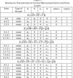
TABLE 1
KINEMATIC PARAMETERS OF LIFTING MECHANISM JOINTS FOR FOUR LOOPS
Pairs Type of the pair i
di i ai sin(i) cos(i)
) (
1АD DF FA
К
0-4 slide 0 d4 0 0 0 1
4-2.2 rotate 22 0 0 а22 0 1
2.2-3 rotate 3 0 0 а3 0 1
) (
2 OB BP PQ QA
К
0-1.2 rotate 12 0 0 а12 0 1
1.2-6.1 rotate 61 0 0 а61 0 1
6.1-9.1 rotate 91 0 0 а91 0 1
) (
3OD DE EC CP PQ QA
К
0-1.1 rotate 11 0 0 а11 0 1
1.1-2.1 rotate 21 0 0 а21 0 1
2.1-7.2 rotate 72 0 0 а72 0 1
7.2-6.2 rotate 62 0 0 а62 0 1
6.2-9.1 rotate 91 0 0 а91 0 1
) (
4OD DE EC CG GL LQ QA
К
0-1.1 rotate 11 0 0 а11 0 1
1.1-2.1 rotate 21 0 0 а21 0 1
2.1-7.1 rotate 71 0 0 а71 0 1
7.1-8 rotate 8 0 0 а8 0 1
8-9.2 rotate 92 0 0 а9 0 1
We obtain the coordinate transformation matrix for circuit K2correspondingly:
.
1 0 0 0
0 1 0 0
0 0
;
1 0 0 0
0 1 0 0
0 0
A ;
1 0 0 0
0 1 0 0
0 0
91 91 91
91
91 91 91 91 2 3
61 61 61 61
61 61 61 61 2 2 12 12 12 12
12 12 12 12 2 1
S a C S
C a S C
A
S a C S
C a S C S
a C S
C a S C
A
The matrix T2 for the loop, mentioned above, will be
equal:
, A
A
2 44 2 43 2 42 2 41
2 34 2 33 2 32 2 31
2 24 2 23 2 22 2 21
2 14 2 13 2 12 2 11
2 3 2 2 2 1 2
t t t t
t t t t
t t t t
t t t t
A
Т (26)
where using the trigonometric functions for sum and differences of angels we simplify elements
t
ij2 for i, j = 1,…,3.
12 61 12 61
91
12 61 12 61
91
12 61 91
2
11 C C S S C C S S C S С
t ;
12 61 12 61 91 12 61 12 61 91 12 61 91
2
12C C S S S C S S C C S
t ;
12 61 12 61 91 12 61 12 61 91 91 12 61 12 61 61 2
14 C C S S C C S S C S a C C S S a
t
12 61 91
61
12 61
12 12 9112
12а a C a C C a
С
;
12 61 12 61
91
12 61 12 61
91
12 61 91
2
21 S C C S C C C S S S S
t ;
12 61 12 61 91 12 61 12 61 91 12 61 91
2
22S C C S S C C S S C C
t ;
12 61 12 61 91 12 61 12 61 91 91 12 61 12 61 61
2
24 S C C S C C C S S S a S C C S a
t
12 61 91
61
12 61
12 1291 12
12a a S a S S a
S
;
0 2 43 2 42 2 41 2 34 2 32 2 31 2 23 2
13t t t t t t t
t ; 2 1
44 2 33t
t .
The coordinate transformation for the circuit K3 could be
. 1 0 0 0 0 1 0 0 0 0 ; 1 0 0 0 0 1 0 0 0 0 ; 1 0 0 0 0 1 0 0 0 0 ; 1 0 0 0 0 1 0 0 0 0 A ; 1 0 0 0 0 1 0 0 0 0 91 91 91 91 91 91 91 91 3 4 62 62 62 62 62 62 62 62 3 4 72 72 72 72 72 72 72 72 3 3 21 21 21 21 21 21 21 21 3 2 11 11 11 11 11 11 11 11 3 1 S a C S C a S C A S a C S C a S C A S a C S C a S C A S a C S C a S C S a C S C a S C A
The final transformation matrix T3assumes the form:
, А А 3 44 3 43 3 42 3 41 3 34 3 33 3 32 3 31 3 24 3 23 3 22 3 21 3 14 3 13 3 12 3 11 3 5 3 4 3 3 3 2 3 1 3 t t t t t t t t t t t t t t t t А А A
Т (27)
where 3
11 21 72 62 91
11С t ;
11 21 72 62 91
3
12S
t ;
11 21 72
21
11 21
11 11;72 62 72 21 11 62 91 62 72 21 11 91 3 14 С а C а C a C a C a t
11 21 72 62 91
3
21S
t ;
11 21 72 62 91
3
22 C
t ;
11 21 72
21
11 21
11 11;72 62 72 21 11 62 91 62 72 21 11 91 3 24 S а S а S a S a S a t 0 3 43 3 42 3 41 3 34 3 32 3 31 3 23 3
13t t t t t t t
t ; 3 1
44 3 33t
t .
The transformation matrices for points D and E of the circuit K4 are similar, i.e. 13
4
1 А
А and 3
2 4
2 А
А . The elementary motion for coordinate systems associated with points С, G, L and Q can be written as:
. 1 0 0 0 0 1 0 0 0 0 ; 1 0 0 0 0 1 0 0 0 0 A ; 1 0 0 0 0 1 0 0 0 0 92 92 92 92 92 92 92 92 4 5 8 8 8 8 8 8 8 8 4 4 71 71 71 71 71 71 71 71 4 3 S a C S C a S C A S a C S C a S C S a C S C a S C A
The transformation matrix Т4 is calculated in the same
way: , А А 4 44 4 43 4 42 4 41 4 34 4 33 4 32 4 31 4 24 4 23 4 22 4 21 4 14 4 13 4 12 4 11 4 5 4 4 4 3 4 2 4 1 4 t t t t t t t t t t t t t t t t А А A
Т (28)
where t114 С
112171892
;
11 21 71 8 92
4
12S
t ;
11 21 71
21
11 21
11 11;71 8 71 21 11 8 92 8 71 21 11 92 4 14 С а C а C a C a C a t
11 21 71 8 92
4
21S
t ; 4
11 21 71 8 92
22C
t ;
11 21 71 21 11 21 11 11; 71 8 71 21 11 8 92 8 71 21 11 92 4 14 S а S а S a S a S a t 0 3 43 3 42 3 41 3 34 3 32 3 31 3 23 3
13t t t t t t t
t ; 3 1
44 3 33t
t .
Because the result of matrices (27) and (28) for loops K3
and K4are equal, we find the joint Q position of the output
link in the local coordinate system of the triangle beam ODB by equaling the corresponding elements of Т3 and Т4
matrix: , ; ; ; ; ; 4 11 3 11 24 4 11 3 11 14 2 11 1 11 22 2 11 1 11 21 1 11 2 11 12 2 11 1 11 11 f C f S b f S f C b f S f C b f C f S b f S f С b f S f С b (29)
where f1C
21726291
C2171892
;
21 72 62 91
21 71 8 92
2 S C
f ;
72 21 72 8 71 21 8 62 72 21 62 92 8 71 21 92 91 62 72 21 91 3 C a C a C a C a C a f
21 71
;71
a C f4a91S
21726291
21 71 8
72
21 72
71
21 71
.8 62 72 21 62 92 8 71 21 92 S a S a S a S a S a
T-transformation which relates to the output link PQL defines coordinate system origin with the position vector
Тz y x p p
p
p , , where T – transpose operation. The orientation of the working body of the lifting mechanism in space is defined by the unit vector (а, о, n) directed along the system Px9y9z9. Thus, the matrix T can be written as:
1 0 0 0 Z Z Z Z Y Y Y Y X X X X i p a o n p a o n p a o n
T . (30)
To find the difference between the elements of the matrices (23) to the corresponding elements of matrix (28) we equal them to the elements of matrix (29). As a result we obtain twelve equations for calculation the vector of the angle and movement in the joint:
. 0 a a o n ; 1 ; ; ; ; ; ; z y x z z 12 12 61 12 61 24 91 61 12 14 91 61 12 91 12 12 61 12 61 24 91 61 12 14 91 61 12 91 22 91 61 12 12 91 61 12 22 91 61 12 12 91 61 12 21 91 61 12 11 91 61 12 21 91 61 12 11 91 61 12 p a p S a S a b S C b С S a p C a C a b S S b С С a o b C C b С S o b C S b S С n b S C b С S n b S S b С С z y x y x y x (31)Substituting in the first and third equation of the system (31) to the expression (29), we determine the formula for b11, …, b22:
. ) ( ; ) ( 91 61 12 2 61 12 1 61 12 11 1 61 12 2 61 12 11 91 61 12 1 61 12 2 61 12 11 2 61 12 1 61 12 11 C n f S f С S f S f С С C n f S f С S f S f С С x x
,2 2 3 1
91 61 12 2
91 61 12 3
11
l l l
S o l C
n l
C x x
(32)
,2 2 3 1
91 61 12 2
91 61 12 1
11
l l l
C n l S
o l
S x x
(33)
where l1C
1261
f1S
1261
f2;
12 61
2
12 61
12 C f S f
l ;
12 61
1
12 61
23 C f S f
l .
The resulting solution is unstable due to the following reasons:
function arccos() and arcsin() are inconvenient because the calculation accuracy of their value depends on the argument;
equalities (32) and (33) will be neither determined or given the low accuracy if the trigonometric functions take values close to zero.
We chosen the arctangent function for the computation of the 11 angle since its values belong to the interval
0112:
12 61 91
2
12 61 91
.3
91 61 12 2
91 61 12 1
11 11 1 1
S o l C
n l
C n l S
o l C S tg
x x
x
x (34)
If we denote the denominator of (35) by τ1 and the
numerator by τ2, the angle 11 will be determined by taking
into account the relevant accessories as follow:
. 0 , 0 ,
0 90
-, 0 , 0 ,
0 9 180
-, 0 , 0 ,
0 18 90
, 0 , 0 ,
0 9 0
2 1 11
2 1 11
2 1 11
2 1 11
1 2 11
если если если если
arctg
The analytical expressions for calculation generalized coordinate allow to provide the given working body position of the lifting mechanism. The results of the inverse kinematics will be used to develop a control system of the mechanism.
IV.THE NUMERICAL EXPERIMENT
Numerical solution of the kinematical synthesis and analysis of the lifting mechanism (Fig. 1) is conducted by the mathematical software application Model Vision Studium (MVS). The software application is an integrated graphical environment for quickly creating interactive visual models of complex dynamical systems that conducts computational experiments allowing to set the equation in the usual mathematical form, to obtain the time and the phase diagram, modify, visualize, and get animation of the object of study.
In accordance with the obtained numerical values of the kinematical parameters of the lifting mechanism [5], and mathematical model of kinematic analysis described in Section 2, it simulates operation of the actuator and the visual model.
Figures 3 and 4 show that the travel of the rod in the hydraulic cylinder is 265 mm that leads to lifting of the output lever of the investigated multi-unit linkage to 1803.27 mm. Synthetic scheme and the values of kinematical parameters are obtained by solving the problem of kinematical synthesis. When the generalized coordinates change within the range from 585 mm to 850 mm there are no breaks in the kinematical chain.
100,0 300,0 500,0 700,0 900,0 1100,0 1300,0 1500,0
560,0 610,0 660,0 710,0 760,0 810,0 860,0
lDA, mm S, mm
[image:6.595.322.535.51.344.2]Joint F Joint Е Joint В Joint С Joint G Joint Р
Fig. 3. Diagram of moving joint.
300,0 700,0 1100,0 1500,0 1900,0 2300,0
560,0 610,0 660,0 710,0 760,0 810,0 860,0
lDA, mm SL, mm
Fig. 4. Diagram of motion of the output link.
The angle of heel of the working platform diagram of the multilink planar linkage is shown in Fig. 5.
The results show that the output link of the mechanism has the maximum inclination in 2,51 degrees along the horizontal axis of the mount coordinate system.
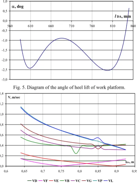
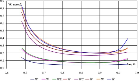
Figures 6 and 7 show the absolute values of analogue of velocity and acceleration of the links and actuator lift mechanism.
-3,0 -2,5 -2,0 -1,5 -1,0 -0,5 0,0 0,5 1,0
560 610 660 710 760 810 860
lDA, mm
[image:6.595.313.538.472.771.2], deg
Fig. 5. Diagram of the angle of heel lift of work platform.
0,0 0,2 0,4 0,6 0,8 1,0 1,2 1,4
0,6 0,65 0,7 0,75 0,8 0,85 0,9 0,95
lDA, m V, m/sec
VD VF VE VB VC VG VP VL
The analysis of the kinematic diagrams of velocity and acceleration of links of the lifting mechanism shows the high quality of motion transmission, the highest values of these characteristics are reached when the stage begins to move.
Fig. 7. Diagrams of values of accelerators of the lifting mechanism.
Fig. 8. The preset position of the actuator
The preset position of the actuator of the lifting mechanism is shown in the fig. 8 setting motion of the working platform
Тx
p
p ,1000,0 . The working body orientation in space with plane-parallel motion of the output link gives the unit vector (а, о, n).
IV. CONCLUSION
Generally, the lifting machines are constructed on the base of scissors lift lever system called Nuremberg scissors and a lifting cargo platform. The key disadvantages of the lifting systems, mentioned above, are the following: limited lifting capacity; low stability at the highest position of the platform; low operation parameters and durability; structure complexity and high material capacity.
The proposed structure of the lifting machine is based on the multi-lever plane mechanism with a changeable closed loop, with increased lateral and longitudinal stiffness providing lifting action by only one hydraulic actuator.
The results of calculation show that the operating platform moves within the vertical working area from 0,3 m through 1,8 m. The parallel level motion of the platform has a negligible inclination in 2,51 degrees and does not impact the operational capacity of the system. The estimated load capacity of the proposed mechanism is up to 200 kg. It can
be folded for transportation and used for both internal and external construction work.
The kinematic characteristics of the lifting mechanism designed in this paper are necessary not only to assess the quality of the synthesis scheme of the mechanism, but also for solving problems related to the strength calculation and construction of its parts, evaluating the dynamic properties of a mechanism that will be the subject of further researches.
REFERENCES
[1] Dzholdasbekov Yu. A Theory of mechanisms of high grades. - M of Education and Science of the Resp. Kazakhstan, Institute of Mechanics and Engineering. - Almaty: Gylym, 2001. - 427s.
[2] Baygunchekov J.J., Dzholdasbekov S. W., Nurakhmetov B.K. Principle of formation of spatial mechanisms regulated high classes. Proceedings of the International Scientific and Technical Conference "Problems and prospects of the development of science and technology in the field of mechanics, geophysics, oil, gas, energy and chemistry of Kazakhstan. "- Aktau, 1996. - 75 p.
[3] Sarkisian Yu. L. The theory of the synthesis of planar linkages using a quadratic approximation. Proceedings of the Academy of Sciences of the Armenian SSR. A series of technical sciences, 1976 – №6. –pp. 4 -9.
[4] Zhursenbaev B. I, Sarbasov T. A. Innovation patent "Jack scaffold" №
22439, issued by the Committee on Intellectual Property Rights, Ministry of Justice of the Republic of Kazakhstan as of 02/25/10. [5] Gebel E.S., Zhursenbaev B. I., Solomin V. Yu. Numerical simulation
of the lifting mechanism Conf. Proc. «9th International Conference On Mathematical Problems In Engineering, Aerospace And Sciences: ICNPAA 2012, Vienna, Austria. : AIP, 2012 – pp. 408-415.
0,0 0,1 0,2 0,3 0,4 0,5 0,6 0,7 0,8 0,9
0,6 0,7 0,7 0,8 0,8 0,9 0,9 1,0