Statistical Inference for a Novel Health Inequality Index

http://www.scirp.org/journal/tel ISSN Online: 2162-2086

ISSN Print: 2162-2078

Statistical Inference for a Novel

Health Inequality Index

Cuizhen Niu

1

_{, Shaoxin Hong}

2

_{, Xuejun Jiang}

3*

1_{School of Statistics, Beijing Normal University, Beijing, China}

2_{Department of Mathematics and Statistics, University of North Carolina, Charlotte, USA}

3_{Department of Mathematics, Southern University of Science and Technology of China, Shenzhen, China}

Abstract

In this paper, we develop statistical inference for an important health inequa-lity index proposed by Lv, Wang and Xu [1] for ordinal data. Asymptotic dis-tributions of the indices are established. This allows us to make inference for the indices. Generalizations of the indices to multiple population setting are also studied. We demonstrate the effectiveness of our procedure using the health inequality data of several areas in Switzerland, and our results classify these areas into three classes based on their health inequalities.

Keywords

Health Inequality Index, Multiple Comparison, Self-Reported Health Status, Statistical Inference

1. Introduction

The qualitative nature of SRHS data prevents the straightforward use of conven-tionally developed indices for measuring income inequality. A reasonable index for SRHS data should be invariant to rescalings of variables which preserve the order of categories.

Assessment on health inequality for ordered data has received attention in the last ten years, [2] and [3] developed median-based concept of inequality. [4] pro- posed polarization measures, which are also median based. These methods are invariant to cardinal scaling on the categories. [5] proposed a method using in-come-health matrix to measure socioeconomic inequality in health. [6] intro-duced a family of sub-group decomposable indices and investigated the decom-posability of the indices. [7] conducted an empirical study of the health inequa-lity index for ordinal data from China. Reference [8] considered the tools and

How to cite this paper: Niu, C.Z., Hong, S.X. and Jiang, X.J. (2017) Statistical Infe-rence for a Novel Health Inequality Index. Theoretical Economics Letters, 7, 251-262.

https://doi.org/10.4236/tel.2017.72021 Received: January 16, 2017

Accepted: February 25, 2017 Published: February 28, 2017 Copyright © 2017 by authors and Scientific Research Publishing Inc. This work is licensed under the Creative Commons Attribution International License (CC BY 4.0).

choices to be made when measuring socioeconomic inequalities with rank-de- pendent inequality indices. [9] made an empirical comparison with several or-dinal and caror-dinal measures of health inequality. [10] proposed a new measure for ordinal health data to monitor income-related health differences between regions in Great Britain. [11] defined a new ratio-scale health status variable and developed positional stochastic dominance conditions that could be imple-mented in a context of multi-dimensionality categorical variables. [12] examined the measurement of social polarization with categorical and ordinal data. [13]

introduced two approaches to measure social polarization in the case where the distance between groups is based on an ordinal variable, such as self-assessed health status. More examples on ordinal inequality measurements can be seen in

[14], [15] and so on. For statistical inference of these recent developed health inequality indices, some authors (e.g. [4], [16]) have derived standard errors for the inequality indices they have introduced. [17] presented a unified methodol-ogy for the estimation of inequality indices of the cumulative distribution func-tion.

Recently, [1] proposed a class of measures of health inequality, which are easy to compute and have some desirable properties, such as additivity, invariance of parallel shifts, normalization and simple aversion to median-preserving spreads. However, it is designed only for one population and has not developed statistical inference for the index. This motivates us to work along this topic. In this paper, we establish asymptotic distributions of the indices introduced by [1] and extend the indices to multiple population settings. Our procedures allow dependence between the considered populations and different sample sizes. In particular, we answer several important questions, for example, whether the health inequality of one population is the same as others and is there a linear relationship among the health inequalities of different populations?

The reminder of the paper is organized as follows. In Section 2, we review the indices developed by [1] and derive asymptotic distribution of the indices. In Section 3, we develop the indices for multiple populations. Empirical results are reported in Section 4. Section 5 concludes the paper.

2. Inference for the Health Inequality Index

2.1. Review of the Indices

According to [1], denote

(

)

T

1, , i, , n

V V V

=

V   as the health statuses of n

in-dividuals. Let

(

)

T

1, , m

h h

=

h  be a finite given set of health categories with

2

m≥ . Assume that health categories represent various health statuses and

sa-tisfy h1<<hm. The values of h1,,hm are ordinally significant so that, if

j k

h <h , then hj represents a lower health status than hk.

Let

(

)

T

1, , m

d d

=

d  and f =

(

f₁,,f_m

)

T be the empirical and population

frequencies of the health categories, respectively, while 1

(

)

1

n

i l l i

d =n−

∑

₌ I V =h

represents the relative frequency of individuals with health statuses equal to hi.

( )

( )

T 0 diag ,

Ω f = f − ff (1)

and let G be a m×m matrix with the

( )

i j, th entry being 2g i

(

− j

)

, where

( )

g ⋅ is a function of nonnegative integers, such that

( )

( )

( )

(

)

0=g 0 <g 1 <g 2 <<g m−1 . Lv, Wang and Xu [1] proposed the

fol-lowing classes of health inequalities:

( )

1

(

)

.

m

i j i j i

I f =

∑ ∑

_{= ≠} g i− j f f (2)

Two typical choices for g

( )

⋅ include the following:

( )

2

( )

1

, 1, , 1; 2 , 1, , 1, 0 1.

1

m i i

g i i m g i i m

m

α

α

− −

= = − = = − < <

−   (3)

Intuitively, the index is estimated by I d

( )

, an empirical plug-in estimator in

statistics.

2.2. Asymptotic Results

Base on the above indices, we establish the following asymptotic distribution. Theorem 1. Using the delta method, we can establish that

( ) ( )

(

)

(

_0, 2

)

_,

n I d −I f ⇒N σ

where 2 T T

( )

0

G G

σ

= f Ω f f .

In practice, σ2 _{is unknown and must be estimated. Given that}

d is a

con-sistent estimator of f , the asymptotic variance can be estimated by

( )

2 T T 0

ˆ G G

σ

=d Ω d d. Based on the asymptotic result, the two-sided symmetric

(

)

100 1−α % asymptotic confidence interval for the health inequality index

( )

I f can be constructed as

( )

( )

(

2 2

)

1 2 ˆ , 1 2 ˆ ,

I d −z_−α σ n I d +z_−α σ n

where z1−α2 is the 1−α 2 quantile of the standard normal distribution.

3. Extension to Multiple Populations

3.1. Testing for Equivalence

We first consider two populations with

(

)

T

1, ,

i = fi fim

f  , d_i =

(

d_i1,,d_im

)

T

and

(

)

T

1, , i , 1, 2

i = Vi Vin i=

V  . Our analysis considers the cases of mutually de-

pendent samples and independent samples, with the former being relevant in examining the evolution of health inequalities in a single group (e.g., changes in health inequality over time), while the latter being relevant in comparing health inequality between two groups (e.g., cross-national). The sampling is performed independently within each group.

Lemma 1. Using the delta method, we have

( ) ( )

(

)

(

)

( )

(

)

(

)

( )

T T

T T 1

1 1

1 p

n

l p

l

n I I n G o

G I V o

n =

− = − +

=

∑

= − +

d f f d f

f h f

matrix. Denote n=max

{

n n1, 2

}

, λi=limn→∞

(

n ni 

)

, 0<λi≤1, i=1, 2 . The

asymptotic distribution of I

( ) ( )

d1 −I d2 is

( ) ( )

(

)

(

( ) ( )

)

(

2 2 2

)

1 2 1 2 0, 11 1 22 2 2 12 1 2 .

n_ I d −I d − I f −I f _⇒N σ λ σ+ λ − σ λ λ

Now we consider hypothesis testing problem,

( )

( )

( )

( )

0,1: 1 2 . . a,1: 1 2 .

H I f =I f v s H I f ≠I f

We introduce the following Wald statistic:

( ) ( )

(

)

2

1 2

2 2 2

11 1 22 2 12 1 2 . 2

n

n I I

T

σ λ σ λ σ λ λ

− =

+ −

d d



(4)

Then under the null hypothesis H0,

2 1

n

T ⇒ as n→ ∞. The

correspond-ing p-value can be computed by the following formula:

(

)

2

( )

1

1 ,

obs obs

p=Pr T ≥t = −F t

 (5)

where 2

( )

1

F ⋅

 represents the cumulative distribution function of the chi-squared variable with one degree of freedom.

These results are general, an assumption of independent populations is not required, this implies that our test work with the unbalanced designs case. If these two populations are treated as independent, then

(

) (

)

{

1 2

}

Cov I Vl ,I Vl 0

τ

=h =h = and thus 2

12 0

σ = . For a particular

circums-tance, when the sample sizes of these two populations are equal, n1=n2=n, we

can have λ1=λ2 =1 and then the asymptotic distribution in Theorem 2

reduc-es to

( ) ( )

(

)

(

( ) ( )

)

(

2 2 2

)

1 2 1 2 0, 11 22 2 12 .

n_ I d −I d − I f −I f _⇒N σ +σ − σ (6)

We propose statistical inference procedures to test the equality between sam-ples in terms of their health inequality indices. This equality issue often emerges when checking for the similarity of the health inequalities in the whole country or in a specified region. For example, China, a country consists of many admin-istrative regions, such as Eastern China, North China, and Central Region, with each region having several provinces. Those provinces in the same region have similar economic and/or social behaviors. Therefore, those provinces in the same region are assumed to have the same health inequalities. We also examine whether the health inequality index of a province is the same as the average in-dex of the entire region. The above two testing problems lead to another applica-tion. If the preceding analysis reveals that the provinces within each region have equal indices, then we can check whether the common means in two regions are also the same. Accordingly, we cluster the regions based on the test results. In other words, if several regions have the same health inequality, then we can view these regions as one cluster.

3.2. Global Test

(

)

T 1, ,

i = di dim

d  and

(

₁, ,

)

T, 1, ,

i

i= Vi Vin i= r

V   . For the dependent sam-

ples, we can obtain the similar results as those presented in Section 2. However, the covariance structure becomes too complex to be practical when more sam-ples are used. We only consider independent samsam-ples for simplification. A global test can be constructed as:

( )

( )

( )

( )

0,2: 1 r . . a,2: i j

H I f ==I f v s H I f ≠I f (7)

for some i≠ j i j

(

, =1, 2,,r

)

.

Define the matrix R=I( ) ( )r− × −1 r1,−L( )r− ×1 1, where I( ) ( )r− × −1 r1 is an identity

matrix with r−1 dimension, and L_{( )r− ×1 1} is a r−1 dimensional vector with

all the elements being 1. Then, Hypothesis in (7) can be rewritten as follows:

( )

( )

0,3: 0, . . a,3: 0,

H RI f = v s H RI f ≠

where

( )

(

( )

( )

)

T

1 , , r I f = I f  I f .

Define n=max

{

n i_i, =1,,r

}

, λ_i=lim_n→∞

(

n n_i 

)

, 0<λ_i≤1, i=1,,r .

Given the independence of the r groups of samples, we can obtain

( ) ( )

(

)

( )

0, ,

n I d −I f ⇒N Σ

 (8)

where

(

2 2

)

11 1

diag σ λ, ,σ λ_{rr r}

Σ =  . Therefore,

( )

( )

(

)

(

_0, T

)

n RI d −RI f ⇒N R RΣ

and

( )

( )

(

)

T

(

_T

)

1

(

( )

( )

)

₂

1. r

n RI d −RI f R RΣ − RI d −RI f ⇒− (9)

Note that under the null hypothesis, RI

( )

f =0 in (9). Consequently, a Wald

type of test statistic can be defined as

( )

(

)

1

( )

T T _ˆ T _,

r

T =nI d R R RΣ − RI d (10)

where

(

2 2

)

11 1

ˆ _{diag ˆ , , ˆ}

rr r

nσ n nσ n

Σ =    is an estimator of Σ_{. Given the central}

role of the test statistic Tr, we state the asymptotic behavior of Tr under the

null hypothesis in the following theorem.

Theorem 3. Let n=max

{

n i_i, =1,,r

}

, λ_i=lim_n→∞

(

n n_i 

)

, 0<λi≤1, 1, ,

i=  r, then under the null hypothesis H_0,1:I

( )

f₁ ==I

( )

fr in (7), we

have 2

1.

r r

T ⇒₋

The corresponding p-value can be computed by:

(

)

2

( )

1

, 1 , ,

r

r r obs r obs

p Pr T t F t

−

= ≥ = − _{ (11)}

where 2

( )

1

r

F − ⋅

 represents the cumulative distribution function of the chi-squared variable with r−1 degrees of freedom. The equality hypothesis (7) can be

re-garded as a generalization of the two-sample comparison case. The availability of this hypothesis can be seen clearly in our empirical application.

3.3. Hypothesis Testing within a Cluster

inequality of a specified population is the same as the average health inequality of entire population. For instance, one may interest to investigate the health in-equality level in Hebei province is higher or lower than the average level of all provinces in the North China region. Accordingly, we propose the following testing hypothesis:

( )

( )

( )

( )

0,4: j 0 . . a,4: j 0

H I f =I f v s H I f ≠I f (12)

for some j j

(

=1, 2,,r

)

. If the null hypothesis H0,1 in (7) holds, then null

hypothesis H0,4 holds naturally. In other words, hypothesis H0,4 only becomes

meaningful when hypothesis H0,1 is not true.

Define

(

)

T

1 , , 1 ,1 1 , 1 , , 1

j= − r − r − r − r − r

a   , that is, a_j is a r×1

vector with its j-th element being 1 1− r and other elements all being −1r.

Hypothesis (12) can be rewritten as follows

( )

( )

T T

0,4: j 0, . . a,4: j 0.

H a I f = v s H a I f ≠

Recall that n I

(

( ) ( )

d −I f

)

⇒N

( )

0,Σ in (8) holds, we can obtain

( )

( )

(

T T

)

(

T

)

0, .

j j j j

n a I d −a I f ⇒N a Σa



Similar to the derivation of Tr, we can construct the following test statistic

( )

(

)

1

( )

T T T _.

j

ra j j j j

T =nI d a a Σa − a I d (13)

Under the null hypothesis in (12), 2

( )

1

j

ra

T ⇒ . Then the p-value can be

determined similarly as that for Tr.

3.4. Hypothesis Testing between Clusters

Further, we discuss the hypothesis testing between clusters. Assume now that our preliminary analysis reveals that the provinces the corresponding region (cluster), such as Eastern China region, have the same health inequality indices. We may then examine whether the health inequalities between two regions are similar. To this end, we choose two representative provinces in each region and then compare their health inequality indices following the proposed approaches in Section 2. However, this method does not employ all information in these groups. To use all underlying information, we compare the common means of these two regions. We consider the following hypothesis:

( )

( )

( )

( )

0,5: 01 02 versus a,5: 01 02

H I f =I f H I f ≠I f (14)

where

( )

1

( )

01 i1 i 1

I f =

∑

τ₌ I f r and

( )

1 2

( )

1

02 1 2

r i i r

I f =

∑

τ +_{= +} I f r .

Without loss of generality, we assume that the first r1 populations are

clus-tered in one group with a common health inequality I f

( )

01 , while the r1+1

to r1+r2 populations are clustered in another group with another common

health inequality I f

( )

02 . H0,5 only becomes meaningful when null

hypothe-sis H0,1 in (7) is not true. Define

(

)

T

1 1 2 2

1 ,r ,1 , 1r r, , 1r, 0, , 0 .

= − −

That is, b is a r×1 vector with its first r1 elements being 1r1, the r1+1

to r1+r2 elements being −1r2 and the other elements being 0. Similar to the

derivation of Tra, we can construct the test statistic as follows:

( )

(

)

1

( )

T T T

. rb

T =nI d b b Σb − b I d (15)

Under the null hypothesis in (14), 2

( )

1 rb

T ⇒ , thus p-value can be

deter-mined similarly as that for Tr.

4. Empirical Application

To illustrate our proposed procedures, we present a real application by using the data of the Swiss Health Survey [SHS] in 2002, conducted by Switzerland's Fed-eral Statistical Office. A total of 19,706 observations were collected from seven areas in Switzerland. The survey respondents were asked to rate their health sta-tuses on a five-point scale ranging from very bad to very good. This dataset was also analyzed by [3] and [6]. We do not include the distributions of SHS in the seven regions in this paper, this information can be found in [6]. We use the health inequality indices proposed by [1] to analyze the survey data and yield new observations. Denote the index with g i

(

− j

)

=2i− j

(

m−1

)

by F1 and

the index with

(

)

1

2 m i j

g i− j =

α

− − − by F2. For checking the robustness of the

results obtained, we choose

α

=0.9, 0.6 and 0.3, then these related indices are

denoted as F2-1, F2-2 and F2-3, respectively.

Table 1 presents the health inequalities of seven areas in Switzerland based on F1 and F2 with different α_{. The standard errors are enclosed in parentheses,}

[image:7.595.212.538.592.735.2]

and the health inequalities are ranked based on the proposed measures. From this table, in all four different measures, we can find that Leman is the region with the highest health inequality value, which implies that the health status ex-ists the most significant difference between Leman citizens. The other regions show ambiguous ranking. Specifically, for F1 and F2-2, Zurich is the region with least difference in health status, and Central has the second-to-the-lowest in-equality. However, for F2-3, Central is identified as the least imbalanced region in health status, while Zurich has the second-to-the-lowest inequality. East and Ticino show the similar behavior.

Table 1. Health inequality in the seven statistical areas of Switzerland.

Area F1 F2-1 F2-2 F2-3

[image:8.595.212.540.606.733.2]

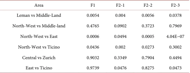
Due to the reason of random sampling of the data set, it is natural to ask ques-tions, like, do East and Ticino have different health inequalities in fact? Do Cen-tral and Zurich have the same health inequality actually? We use statistical infe-rences to address these problems. To fully answer these questions, various inter-esting two-sample comparison tests are carried out, the results are reported in

Table 2. We set the significance level to 5%. From Table 2, we can conclude

that Leman is significantly more imbalanced than Middle-Land in health status. In contrast to the findings in Table 1, Middle-Land and North-West do not show statistically significant differences in their health inequalities. In other words, these two regions have the same health inequality level base on the data set we have. North-West is significantly more unbalanced in health status than East. Except for F2-3, all p-values for North-West and Ticino are all smaller than

5%. Therefore, the difference of health inequality between North-West and

Ti-cino can be confirmed almost. Central and Zurich have the same inequality level, and the same finding has been observed for East and Ticino.

Based on the above analysis, we classify North-West and Middle-Land, East and Ticino, and Central and Zurich into three groups. However, can we com-bine two groups, such as the East and Ticino group with the Central and Zurich group? The question is equivalent to ask whether the average health inequality of the East and Ticino group is the same as that of the other group. The p-values of tests by using the above four measures are 0.5505, 0.1778, 0.7105 and 0.0140, re-spectively, which are all larger than 5% except for F2-3. Therefore, East, Ticino,

Central, and Zurich may be clustered into one group. We also check whether these four regions have the same health inequality levels. The p-values for this global equality hypothesis testing are 0.8805, 0.1824, 0.8946 and 0.0942, respec-tively, which suggest that these regions have the same inequality levels. We then examine whether this four-member group can be enlarged by including the North-West and Middle-Land group? We propose two hypotheses to investigate this question. First, are the average inequalities of North-West and Middle-Land similar to those of the other groups? Second, do these six regions have the same health inequality levels? For these two hypotheses, all the p-values resulting from tests with the four measures are significantly smaller than 5%, which indicate

that the average health inequality of the North-West and Middle-Land group is different from that of the four-member group. We then examine whether the

Table 2.p-values for two-sample comparison problems.

Area F1 F2-1 F2-2 F2-3

Leman vs Middle-Land 0.0054 0.004 0.0056 0.0378 North-West vs Middle-land 0.4765 0.0902 0.3723 0.7969 North-West vs East 0.0006 0.0494 0.0005 4.04E−07 North-West vs Ticino 0.0436 0.002 0.0273 0.3002

health inequality level of Leman is the same as the average level of the North- West and Middle-Land group. The p-values of all four measures are strongly smaller than 5%, which indicate that the health inequality level of Leman is

different from the average level of the North-West and Middle-Land group. In sum, we classify these seven regions into three groups, that is, Leman, North- West and Middle-Land, and the other four regions.

5. Conclusion

In this paper, we propose several statistical inference procedures for the novel health inequality indices introduced in [1]. We consider one-, two-, and mul-tiple-sample cases. Given that health surveys generally cover multiple regions, the health inequalities of multiple sample cases must be tested. The health in-equality in various regions of Switzerland validates the availability of our pro-posed tools. Seven regions covered by SHS can be categorized into three groups after the numerical study; Leman has the highest health inequality followed by the North-West and Middle-Land group. The other four regions (i.e., Central, East, Ticino, and Zurich) have the same health inequality. Our proposed proce-dures can also be applied to other recently proposed health inequality indices. The subjective well-being is influenced by many factors such as health inequality, education, environment and so on. The statistical inference on multi-dimen- sionality well-being inequality can be investigated ongoing.

Acknowledgements

This research was funded by the Fundamental Research Funds for the Central Universities, China Postdoctoral Science Foundation (2016M600951), National Natural Science Foundation of China (11101432) and Natural Science Founda-tion of Guangdong Province, China (2016A030313856). The authors thank the editor, the associate editor and the anonymous referee for their constructive comments and suggestions which led to a substantial improvement of an early manuscript. All correspondence should be addressed to Xuejun, Jiang, Depart-ment of Mathematics, Southern 6 University of Science and Technology, Shenz-hen, China, E-mail: [email protected].

References

[1] Lv, G. M., Wang, Y. and Xu, Y. S. (2015) On a New Class of Measures for Health Inequality Based on Ordinal Data. The Journal of Economic Inequality, 13, 465-477.

https://doi.org/10.1007/s10888-014-9289-4

[2] Allison, R.A. and Foster, J.E. (2004) Measuring Health Inequalities Using Qualita-tive Data. Journal of Health Economics, 23, 505-524.

https://doi.org/10.1016/j.jhealeco.2003.10.006

[3] Abul Naga, R.H. and Yalcin, T. (2008) Inequality Measurement for Ordered Re-sponse Health Data. Journal of Health Economics, 27, 1614-1625.

https://doi.org/10.1016/j.jhealeco.2008.07.015

[4] Apouey, B. (2007) Measuring Health Polarization with Self-Assessed Health Data.

[5] Zheng, B. (2011) A New Approach to Measure Socioeconomic Inequality in Health.

The Journal of Economic Inequality, 9, 555-577.

https://doi.org/10.1007/s10888-010-9148-x

[6] Kobus, M. and Miloś, P. (2012) Inequality Decomposition by Population Subgroups for Ordinal Data. Journal of Health Economics, 31, 15-21.

https://doi.org/10.1016/j.jhealeco.2011.11.005

[7] Wang, H.L. and Yu, Y.W. (2016) Increasing Health Inequality in China: An Empir-ical Study with Ordinal Data. The Journal of Economic Inequality, 14, 41-61.

https://doi.org/10.1007/s10888-015-9315-1

[8] Erreygers, G. and Van Ourti, T. (2011) Measuring Socioeconomic Inequality in Health, Health Care and Health Financing by Means of Rank-Dependent Indices: A Recipe for Good Practice. Journal of Health Economics, 30, 685-694.

https://doi.org/10.1016/j.jhealeco.2011.04.004

[9] Madden, D. (2010). Ordinal and cardinal measures of health inequality: an empiri-cal comparison. Health Economics, 19, 243-250. https://doi.org/10.1002/hec.1472

[10] Allanson, P. (2017) Monitoring Income-Related Health Differences between Re-gions in Great Britain: A New Measure for Ordinal Health Data. Social Science and Medicine, 175, 72-80. https://doi.org/10.1016/j.socscimed.2016.12.033

[11] Makdissi, P. and Yazbeck, M. (2014) MEASURING Socioeconomic Health Inequa-lities in Presence of Multiple Categorical information. Journal of Health Economics, 34, 84-95. https://doi.org/10.1016/j.jhealeco.2013.11.008

[12] Permanyer, I. and D’ambrosio, C. (2015) Measuring Social Polarization with Or-dinal and Categorical Data. Journal of Public Economic Theory, 17, 311-327.

https://doi.org/10.1111/jpet.12093

[13] Fusco, A. and Silber, J. (2014) On Social Polarization and Ordinal Variables: The Case of Self-Assessed Health. The European Journal of Health Economics, 15, 841- 851. https://doi.org/10.1007/s10198-013-0529-5

[14] Erreygers, G. (2009) Correcting the Concentration Index. Journal of Health Eco-nomics, 28, 504-515. https://doi.org/10.1016/j.jhealeco.2008.02.003

[15] Lazar, A. and Silber, J. (2013) On the Cardinal Measurement of Health Inequality When Only Ordinal Information Is Available on Individual Health Status. Health Economics, 22, 106-113. https://doi.org/10.1002/hec.1821

[16] Cowell, F. and Flachaire, E. (2014) Inequality with Ordinal data. Unpublished. [17] Abul Naga, R.H. and Stapenhurst, C. (2015) Estimation of Inequality Indices of the

Cumulative Distribution Function. Economics Letters, 130, 109-112.

Appendix. Proofs of Theorems

Proof of Theorem 1.

Given that d is a consistent estimator of f , for the empirical frequency of

the health categories, we can easily obtain the following:

(

)

(

0, 0

( )

)

,

n d− f ⇒N Ω f (A.1)

where

( )

( )

T

0 diag .

Ω f = f − ff

Note that g i

(

− j

)

f fi j=g

(

j−i f f

)

j i. Therefore,

( )

1

(

)

1 1

2 .

m m

i j i j i

I g i j f f

−

= = +

=

∑ ∑

−

f

Define

( )

( )

T 1 , , m I I J f f ∂ ∂   =  _{∂ ∂}    f f

 It can be easily shown that

( )

₍

₎

2 _l.

l i i

I

g l i f

f ≠ ∂ = − ∂

∑

f (A.2)

Alternatively, we can have J =Gf . Keeping only the first two terms of the

Taylor expansion, we can estimate I f

( )

as

( ) ( )

T

(

)

. I d ≈I f +J ⋅ d− f

Then the variance of I

( )

d −I

( )

f is approximated by

(

)

(

)

(

)

(

)

T T T T 0

Var Cov ,

.

J J J

G n G

⋅ − = ⋅ − − ⋅

= Ω

d f d f d f

f f

Also E I

(

( )

d

)

=E I

(

( )

f

)

since d is a consistent estimator of f , it

fol-lows that

( ) ( )

(

)

(

2

)

0, ,

n I d −I f ⇒N σ

where 2 T T

( )

0

G G

σ

= f Ω f f .

Proof of Theorem 2.

Define n=max

{

n n1, 2

}

, λi=limn→∞

(

n ni 

)

, 0<λi≤1, i=1, 2. From Lemma

1, we have

( ) ( )

(

)

(

)

( )

(

)

(

)

( )

T T T T 1 1 1 1 . p n l p l

n I I n G o

G I V o

n =

− = − +

=

∑

= − +

d f f d f

f h f

Let 2

(

(

) (

T

)

)

1 2

Cov

h I Vl I Vl

σ = =h =h . After that, similarly as the proof of

Theorem 1, it can be derived that

( ) ( )

( ) ( )

( ) ( )

(

)

( ) ( )

(

)

(

)

(

)

(

)

(

)

( )

1 2 T T

1 1 1

1 1 1 1

1

1 1

1 1

2 2 _{T T}

2 2 2 1 2 2 2

2 2 2

2 2

11 1 12 1 2

2 2

21 1 2 22 2

1 1 1 0 , . 0 n l l p n k k n n

G I V

n I I

n

n n

I I

n o

I I _{n n}

n I I G I V

n n n

N σ λ σ λ λ

σ λ λ σ λ

= =     × = − × −      − ₌ ₌ ₊  ₋  _{   }   _{ × −   × = − }         _{ }      ⇒ _{  }  _{   }  

∑

∑

f h f

d f

d f

d f

d f f h f

 



 

Here,

( )

(

) (

)

(

)

( )

2 T T

11 1 0 1 1

2 2 T T T T T 2

12 21 1 1 2 2 1 2

2 T T

22 2 0 2 2 ,

Cov l l h ,

G G

G I V I V G G G

G G

σ

σ σ σ

σ

= Ω

= = = = =

=

f f f

f h h f f f

f f f

Plug in the consistent estimators of fi and 2

h

σ by di and

(

)

{

}

₁min{1,2}

(

) (

)

2 T T

1 2 1 2 1 2

1

ˆ min , ,

n n

h l l

l

n n I V I V

σ −

=

=

∑

=h =h −d d

respectively, thus we can easily estimate 2

, , , 1, 2 i j i j

σ

= _{consistently.}

Combining the above result in (A.3), we can obtain

( ) ( )

(

)

(

( ) ( )

)

( ) ( )

(

)

(

( ) ( )

)

(

)

1 2 1 2

1 1 2 2

2 2 2

11 1 22 2 12 1 2

0, 2 .

n I I I I

n I I I I

N σ λ σ λ σ λ λ

 − − − 

 

 

= _ − − − _

⇒ + −

d d f f

d f d f





Submit or recommend next manuscript to SCIRP and we will provide best service for you:

Accepting pre-submission inquiries through Email, Facebook, LinkedIn, Twitter, etc. A wide selection of journals (inclusive of 9 subjects, more than 200 journals)

Providing 24-hour high-quality service User-friendly online submission system Fair and swift peer-review system

Efficient typesetting and proofreading procedure

Display of the result of downloads and visits, as well as the number of cited articles Maximum dissemination of your research work

Submit your manuscript at: http://papersubmission.scirp.org/