Munich Personal RePEc Archive
Agriculture, Predation and Development
Bethencourt, Carlos and Perera-Tallo, Fernando
Universidad de La Laguna
10 October 2012
Online at
https://mpra.ub.uni-muenchen.de/41919/
Agriculture, Predation and Development
1Carlos Bethencourt Fernando Perera-Tallo Universidad de La Laguna Universidad de LaLaguna
Abstract: Predation attracts a relatively high portion of labor in developing countries and obstructs development. Agriculture also has an important weight in employment in these countries. We formulate a model in which agents devote time either to predation or to producing agricultural and manufactured goods with the following features: a subsistence level of agricultural goods must be reached and, consequently, poor countries devote more resources to agriculture; agriculture is more land intensive and, thus, has a lower labor share than manufacturing; and incentives to devote time to production increase with the labor share. The share of manufactured goods in GDP increases throughout the transition, raising the labor share, which discourages predation and fosters production. This mechanism involves an amplification effect of the differences in productivity among countries due to the reallocation of labor from predation to production. Institutional quality plays a crucial role in this process, since it discourages predation.
1We thank the participants at the XVI conference on Dynamics, Economic Growth, and International
Trade (DEGIT-XVI) held in the SPbU Saint Petersburg for their helpful comments. We specially thank
José-Víctor Ríos-Rull, Alberto Bucci, Jakub Growiec and David Mayer-Foulkes. Both authors are members
I. Introduction
Many developing countries fail to achieve a successful development process (see Quah 1996, 1997 and Parente and Prescott, 1993). Much effort in current macroeconomic research has been devoted to explaining this fact. In particular, new features, such as the nature and composition of the economic activities have been explored. It is well known that in economies, resources are devoted to both productive activities (production of goods and services) and unproductive activities. Unproductive activities entail a group of activities that share the common feature of being profitable, but wasteful: they use resources to generate rents (i.e., income) but not goods (for example, property crime, fraud, begging, lobbying, rent-seeking, etc.). We will call all these unproductive activities predation from now on. Empirical evidence suggests that the size of the unproductive sector is larger in low income countries. For example, the share of the criminal predatory sector in GDP is 20.7% for Latin America, while it is 6.89% for the United States2. Another example in the literature is from Bourguignon (1999), who finds that the share of property crime in GDP is 0.5% for United States, while it is 1.5% for Latin America.
It is widely accepted that the size of the agricultural sector in developing countries is larger than in developed countries. Development literature characterizes the “food problem” as the stage in which a country mustfirst be able to satisfy its own subsistence needs before the transition to economic growth can start to take off. Once the “food problem” is solved, a structural change takes place in which agriculture loses weight throughout the development process.
Many recent studies have found agriculture to be less labor intensive than both industry and services while the capital intensity is similar for all sectors (see Herrendorf and Valentinyi, 2008; and Echevarria, 1999). Thus, since the portion of resources devoted to agriculture is larger in developing countries and labor share in agriculture is smaller than in other sectors, it is reasonable to assume that labor share in developing countries is smaller than in developed countries.
likely that part of their production is not accounted for in the GDP (the denominator of the labor share). In spite of this upward bias in the labor share of developing countries, it still remains lower than in developed countries after the adjustment proposed by Gollin. More precisely, the average labor share of developing countries reported by Gollin is 0.584, while the average in developed countries is 0.6873. One obvious limitation in Gollin’s analysis is the small data set used in which developing countries are under-represented. Harrison (2005) using a similar methodology, but with a much larger data set with respect to both the number of countries and number of years, confirms that there are significant differences in labor share between developing and developed countries, with developing countries displaying lower shares. Another approach is to use industrial data. This approach has the advantage that the weight of the self-employment in the sample is negligible or insignificant. Results show that using such an approach, there exists a clear and positive relationship between labor share and development indicators, such as per capita income (Ortega and Rodriguez, 2006) or capital accumulation (Decreuse and Maarek, 2009; and Maarek, 2010). Thus, all the three empirical methodologies: conventional national account calculation; adjusted national account calculation to incorporate self-employed; and the industrial data approach confirm that developing countries exhibit lower labor shares than developed ones.
This paper introduces a mechanism that connects the empirical facts mentioned above.
3To calculate these averages, we consider developing countries to be those in which the per capita GDP
reported by Gollin was smaller than US $ 6,000 (1985 as basis year) and developed countries as those
above this threshold (GDPs reported by Gollin were mostly from 1992 with 1985 being the basis year).
This classification coincides with the one used by the IMF and the World Bank (the World Bank uses
the terminology low and middle income countries for developing countries and high income countries for
to production. Summarizing, a structural change occurs throughout the transition from an initial per capita capital lower than the steady state level during which predation falls and the weight of agriculture declines in favor of manufacturing.
This paper also offers a new explanation to understand why differences in per capita income among countries have persisted. Conventional wisdom says that differences in TFP are one of the main sources of differences in per capita income4. This paper proposes a mechanism that amplifies differences in TFP and per capita income generated by technolog-ical differences across countries. This mechanism involves the reallocation of resources from predation to productive activities and the incentives to engage in these activities. In this sense, the mechanism is in line with the empirical research that emphasizes the differences in “social infrastructure”, using the terminology by Hall and Jones (1999), to understand diff er-ences in TFP across countries, instead of the more conventional view, which considers these differences as mere technological ones. The mechanism works as follows: when productivity (in manufacturing or agriculture) rises, there is a positive direct effect on production and an indirect effect due to the accumulation of capital (the rise in productivity increases the return on savings and so, the incentives to accumulate more capital). Together with these standard mechanisms, in the current model there is another additional mechanism which amplifies the effect of productivity on per capita income. This new mechanism is related to predation and the change in the sectorial composition so that when productivity rises, the per capita capital rises and resources are reallocated from agriculture to manufacturing. The larger the relative size of the manufacturing sector, the greater the aggregate labor share, reducing the incentive to predate and increasing the portion of labor devoted to production
(agriculture and manufacturing). This increase in the amount of labor devoted to production has three positive effects on the per capita income: )a direct effect on per capita production; ) an indirect effect due to the accumulation of capital: when labor rises, it increases both the marginal productivity of capital and the incentive to accumulate more capital and) a reduction in the portion of labor devoted to predation implies that the share of the marginal product of capital that goes to savers grows, raising the return on savings and promoting the accumulation of capital.
This paper also analyzes the role of institutional quality. We show that institutional quality is a crucial factor for development. In particular, wefind that an improvement in the institutional quality reduces the productivity of predation, generating a labor reallocation from predation to productive activities which produces the same three positive effects on per capita income, as described above.
There is a large amount of literature devoted to the allocation of labor to productive and unproductive activities (see for example, Murphy, Shleifer, and Vishny, 1993, Acemoglu, 1995, Schrag and Scotchmer, 1993, Grossman and Kim, 2002 and Chassang and Padró-i-Miquel, 2010). However, this literature does not deal with the interaction between predation and labor share. Moreover, are also a considerable number of papers on structural transfor-mation which analyze the process of industrialization (see for example Restuccia, Yang and Zhu, 2008, Gollin, Parente and Rogerson, 2002, 2004, 2007, and Córdoba and Ripoll, 2009), though they do not deal with predation.
This paper is organized as follows. Section 2 develops a model of three sectors: agri-culture, manufacturing and predation. Section 3 analyzes agents’ decisions and section 4 defines the equilibrium. Section 5 explains how the labor share and predation evolve with the per capita capital level. Section 6 presents the dynamic behavior of the economy. Sec-tion 7 analyzes how predaSec-tion amplifies differences in productivity across countries and the role of institutions. The last section, section 8, concludes and appendix presents proofs and technical details.
II. The model
investment in physical capital:
() =() + () +() (1)
where () denotes the aggregate production in manufacturing, () denotes the aggre-gate consumption in manufacturing, () denotes aggregate capital and ∈ (01) denotes depreciation rate. () +() is the gross investment.
A. Technology
Production technologies of agricultural and manufactured goods are given by the following production functions:
() = Γ(())(())(())1−− (2)
() = Γ(())(())1− (3)
where () and () denote, respectively, the physical capital used in agriculture and manufacturing; ()and ()the amount of labor used in agriculture and manufacturing, and() denotes the amount of land used in agriculture. In order to capture the fact that
B. Preferences
There are many identical dynasties with “infinite life”. To simplify, we assume that popula-tion is constant. Preferences of a dynasty are given by the following funcpopula-tion:
Z ∞
ln (()−)−(−) () =
⎧ ⎪ ⎪ ⎨ ⎪ ⎪ ⎩
() if ()≤ +() if ()≥
where () and () denote, respectively, the per capita consumption of dynasty of agri-cultural and manufactured goods in period , and 0 is the discount rate of the utility function. Thus, these preferences imply a “food problem”: households do not consume man-ufactured goods until reaching a certain “subsistence” level of consumption of agricultural goods, denoted by.
C. The predation technology
Each period, agents are endowed with units of land and one unit of time, which can be devoted to undertaking two types of economic activities: to produce goods and to commit predation , that is,
1 =() +() (4)
We consider that predation activities are all activities which imply use of resources to obtain incomes without generating production. We include property crimes, fraud, corruption, lobbying, etc. The amount of income obtained through predation is denoted by e()(), where e() is the per capita production and : <+ → [01] is the fraction of per capita
concave, continuous and differentiable of the second order and (0) = 0, (1) 1 and 0(0)≥1.
III. Agents’ decisions
We will concentrate on the case in which consumption is above subsistence level and therefore consumption of manufactured good is positive.
A. Households:
Household maximization problem is as follows:
{()()()()}∞=0
Z ∞
0
ln(())− (5)
:
() = ()()+()()+()-(e())()
| {z }
Net income from production
+ (())e()
| {z }
Predation income
-()-()
() +() = 1
() = ()() + (+())() +()
where()denotes the amount of assets of the household,()the wage per unit of labor,()
the net return on assets, () the renting price of land, () the household’s gross income and() the price of agricultural goods in terms of manufactured goods. We normalize the
predation and e the per capita gross income. Income coming from the production sector is equal to labor income from the production sector()() plus financial income ()(), plus land rents (), minus the amount of this income that is predated by other agents in
the economy(e())(). The other source of income comes from the predation sector which
is equal to(())e(). It is quite obvious from the preferences definition that when an agent enjoys a consumption level above the subsistence consumption level, she is going to consume the subsistence level of agricultural goods . Thus, the total expenditure in consumption is equal to the expenditure in agricultural goods, (), plus the expenditure in consumption of manufactured goods (). The increase of the household’s assets, (), is equal to its savings, which is equal to its income (the one from production plus the one from predation) minus the expenditure in consumption goods, () +().
The first order conditions for the interior solution are as follows:
()h1−(e())
i
= 0(())e() (6)
()
() =
(() +)³1−(e())´−− (7)
Equation 6 specifies that the net wage in the production sector after predation should be equal to the marginal payment of predation activities. That is, the marginal payment of the time devoted to each activity should be equal. Equation (7) is the typical Euler equation. The speed at which consumption grows depends positively on the return on savings,(() +
)³1−(e())´− and negatively on the discount rate of the household, . The following transversality condition should also be satisfied:
lim →+∞
1
()
B. Firms:
Firms maximize profits:
max
−−−(+)
: Γ1−− ≥
(8)
max
−−(+)
: Γ1− ≥
(9)
where factors are measured in per capita terms. The first order conditions of the above problems are:
(1−−)Γ
1−−
= (10)
Γ
1−−
= (+) (11)
Γ
1−−
= (12)
(1−)Γ
1−
= (13)
Γ
1−
= (+) (14)
These conditions are well known and indicate that firms hire a factor until reaching the point at which the marginal productivity of the factor is equal to its price. The per capita production of the agricultural and manufacturing sectors are:
= Γ1−− (15)
IV. Equilibrium Definition
The definition of equilibrium is standard: equilibrium occurs when agents maximize their objective functions and markets clear. Steady state equilibrium is an equilibrium in which both the allocation and prices always remain constant over time.
Definition 1 An equilibrium is an allocation {() () () () () () ()
() () () () ()e()e()
o∞
=0 and a vector of prices{() () () ()}
∞
=0
such that ∀ the following conditions hold:
• Households maximize their utility, that is, {() () () ()}∞=0 is the solution of
the household’s maximization problem (5) and() =.
• Firms maximize profits, that is, ∀ (), (), (), () and (), (), () are the solution of the optimization problem offirms (8) and (9).
• Capital market clears: ∀ () +() =() =().
• Labor market clears: ∀ () +() =().
• Land market clears: ∀ () =.
• Good Market clears: =(),() +
() +() =().
• Finally, since households are identical, per capita variables coincide with household variables: ∀ e() =() ande() =()() + (+())() +().
Definition 2 Steady state equilibrium is an equilibrium in which both the allocation and
V. Predation and per capita capital
A. Labor share
We define the labor share, in the productive sector as the fraction of labor income over the value of the production:
=
=
+
+
We denote the portion of productive labor devoted to agriculture by ≡.
Lemma 3 Labor share is a decreasing function of the portion of productive labor devoted to
agriculture, .
Labor share in the economy is a weighted average of the labor share in the manufacturing and agricultural sectors, where the weight of each sector is equal to the portion of the value of production that each sector has in the aggregate GDP. If a higher portion of productive labor is devoted to agriculture, then a higher portion of GDP comes from the agricultural sector, and this reduces labor share.
Lemma 4 The portion of labor devoted to predation, , is a strictly decreasing function of
labor share, with = 1 when = 0and =min ≤1 when = 1.
Thus, a higher labor share increases the relative reward for work with respect to predating, which encourages work in productive activities and discourages predation.
B. Labor devoted to predation and per capita capital
Proposition 5 The portion of labor devoted to agriculture at equilibrium, , and the
and , and a strictly increasing functions of . The portion of labor devoted to production
at equilibrium, is a strictly increasing function of , Γ and , and a strictly decreasing
function of .
Households’ preferences imply that households do not consume manufactured goods until reaching a certain “subsistence” level of consumption of agricultural goods, . When the resources of the economy (per capita capital or land) expand or agricultural technology improves, then more resources, including labor, become available and may be devoted to the manufacturing sector. This increases labor share, discouraging predation and fostering work in productive activities. Exactly the opposite effects occur if the subsistence level of consumption goes down.
From now on, we will denote by () and () and () the functions that relate, respectively, to the amount of labor devoted to predation, the amount of labor devoted to production and the portion of productive labor devoted to agriculture in equilibrium with the per capita capital, .
VI. Dynamic Behavior
The dynamic system that defines the dynamic behavior of the economy is as follows:
() = (())−()−()
()
() = ((()) +) (1−((())))−−
where () is the function that relates per capita production of the manufacturing sector
and others to predation. (()) is the function that relates the interest rate at equilibrium to per capita capital. These two functions are defined in the appendix.
Lemma 6 The production of the manufacturing sector at equilibrium is a strictly increasing
function of the capital: : [min0] → <+. The net interest rate (()) is a strictly
decreasing function of the capital. If (1−)then the gross interest rate after predation
((()) +) (1−((()))) is a strictly decreasing function of the capital.
The above lemma states that the net interest rate that savers receive (after predation) is a decreasing function of per capita capital.
Lemma 7 Ω ∈ <++ exists so that if Γ Ω then, max min 0 exists so that
+¡min¢ and when ∈¡min max¢ then
() .
The above lemma establishes a sufficient condition to guarantee the existence of a steady state in which the consumption of manufactured goods is positive. We assume that Γ Ω Lemma 6 and 7 imply that the net interest rate equalizes the discount rate of the utility just once. Therefore, there is a unique steady state with a positive amount of manufactured goods.
Corollary 8 If (1− ) there is a unique steady state with a positive amount of
consumption of manufactured goods.
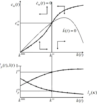
Phase diagram in figure 1 shows that the dynamic behavior of the economy is charac-terized by the typical saddle point dynamic5: there is a unique path which converges to the steady state. This means that, given the initial level of per capita capital, there is a unique equilibrium path, which converges to the steady state. When the initial amount of per capita capital is lower than the steady state level, the consumption and the portion of labor devoted to production grow throughout the equilibrium path, converging to their steady state levels, while the amount of labor devoted to predation goes down. When the amount of per capita capital is larger than the steady state level the opposite happens. Thus, when the starting per capita capital is below the steady state level, there is a “structural change” throughout the transition: there is a reallocation of labor from agricultural and predation sectors to the manufacturing sector, as documented in the empirical literature.
VII. Predation as an amplification mechanism and the role of institutions
A. The effect of an improvement in the technology of the agricultural sector
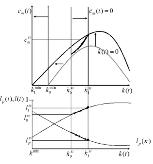
Phase diagram infigure 2 displays the dynamic effect of an improvement in the technology of the agricultural sector,Γ. When there is an improvement in the technology of this sector,Γ,
producing the subsistence level of consumption requires fewer resources. As a consequence, part of the capital and labor devoted to producing the subsistence level of consumption in the agricultural sectorflows to the manufacturing sector, increasing the amount of resources devoted to it. Furthermore, there is an amplification effect due to predation: when the amount of resources devoted to the agricultural sector falls, the labor share of the economy
rises and this encourages the use of labor for productive activities, increasing further the production of the manufacturing sector. This amplification effect involves a rise in the return on savings, due to the fact that the fall in predation has a direct positive effect on the portion of the return on capital that goes to savers, encouraging capital accumulation and moving the locus to the right. The increase in the production of the manufacturing sector is reflected in the movement of the locus, which goes up. As a consequence, the economy moves towards the new steady state with a higher level of capital, a lower portion of labor devoted to predation and a higher portion of labor and capital devoted to manufacturing. Throughout the transition there is a “structural change”: there is a flow of labor from agricultural and predation sectors to the manufacturing sector.
B. The effect of an improvement in the technology of the manufacturing sector
The effect of an improvement in the technology in the manufacturing sector, Γ, is similar
and the increase in productive labor amplify the effect of technological change on capital accumulation. Furthermore, the fall in predation has a direct positive effect on the portion of the return on capital that goes to savers, encouraging additional capital accumulation.
C. The role of institutions
To analyze the role of institutions in the model we make a straightforward extension. We introduce a parameter, , in the predation technology which reduces the productivity of predation, and we interpret such parameter as an index of institutional quality. To be more precise, consider that the amount of income obtained through predation is equal to ( )e(), with ( ) having the same properties defined above but now ()is a strictly
decreasing function of, the index of institutional quality. Thus, the effect of an improvement in institutional quality, , is similar to the improvement in technology analyzed above and displayed in phase diagram infigure 2, but with a jump down in predation and a jump up in productive labor at the moment of change inin the bottom part of thefigure. The economy goes towards the new steady state with a higher level of capital, a lower portion of labor devoted to predation and a higher portion of labor and capital devoted to the manufacturing sector.
VIII. Conclusions
goods before starting to consume manufactured goods. As the country accumulates capital and subsistence needs begin to be satisfied, resources are devoted to manufacturing. This reallocation of factors implies that (aggregate) labor share rises during the transition when the initial per capita capital is lower than the steady state level. This increase in labor share implies a reduction in incentives to predate and a reallocation of labor from predation to production. Thus, this paper not only analyzes how predation affects capital accumulation but also how capital accumulation affects predation and the resulting feedback process.
This paper proposes a mechanism that amplifies the differences in per capita income generated by differences in productivity that shed some light on understanding differences across countries in per capita income. When productivity rises, there is a direct standard effect on production and an indirect standard effect due to the accumulation of capital: the rise in productivity increases the return on savings and thus, the incentives to accumulate more capital. However, in our model, there is an additional mechanism related to the reallocation of resources across sectors and the reduction in predation: when productivity rises, the per capita capital rises, generating a reallocation of resources from agriculture to manufacturing and so, an increase in labor share, which reduces the incentive for predation and increases the portion of labor devoted to production. This increase in the amount of labor devoted to production has three effects: ) a direct effect on per capita production; ) an indirect effect due to the accumulation of capital: when labor rises, it increases the marginal productivity of capital and thus, the incentive to accumulate more capital; )
and promoting further the accumulation of capital.
IX. References
Acemoglu, D. (1995) “Reward Structures and the Allocation of Talent”,European Economic Review, January, 39 (1), 17-33.
Acemoglu, D., Johnson, S. and J.A. Robinson (2005) “Institutions as a Fundamental Cause of Long-Run”, in Handbook of Economic Growth, Volume 1, Part 1, ed. Philippe Aghion and Steve Durlauf, Elsevier.
Anderson, D.A. (1999) “The Aggregate Burden of Crime”, Journal of Law and Eco-nomics, 42 (2), 611-642.
Andonova, V and H. Zuleta (2009) “Beyond Moral Hazard: The Effect of Firm-Level Compensation Strategies on Economic Conflict”,Peace Economics, Peace Science and Public Policy, 15 (1), article 5.
Banerjee, A. and E. Duflo (2007) “The economic lives of the poor. Journal of Economic Perspectives”, 21 (1), 141-167.
Bourguignon, F. (1999) “Crime as a social cost of poverty and inequality: a review focusing on developing countries”, Washington, D.C.-París, World Bank-Delta, mimeo.
Chassang, S. and G. Padró-i-Miquel (2010) “Savings and Predation”, Journal of the European Economic Association, 8 (2-3), 645-654.
Córdoba, J.C. and M. Ripoll (2009) “Agriculture and aggregation”, Economics Letters, 105 (1), 110-112.
Easterly, W. and R. Levine (2001) “It’s Not Factor Accumulation: Stylized Facts and Growth Models”, World Bank Economic Review, 15 (2), 177-219.
Gollin, D. (2002) “Getting Income Shares Right”, Journal of Political Economy, 110 (2), 458-474.
Gollin, D., Parente, S. and R. Rogerson (2002) “The Role of Agriculture in Development”,
American Economic Review, 92 (2), 160-164.
Gollin, D., Parente, S. and R. Rogerson (2004) “Farm Work, Home Work, and Interna-tional Productivity Differences”,Review of Economic Dynamics, 7 (4), 827-850.
Gollin, D., Parente, S. and R. Rogerson (2007) “The food problem and the evolution of international income levels”, Journal of Monetary Economics, 54 (4), 1230-1255.
Grossman, H.I. and M. Kim (2002) “Predation, Efficiency, and Inequality”, Journal of Institutional and Theoretical Economics, 158 (3), 393-407.
Hall, R.E. and C.I. Jones (1999) “Why do Some Countries Produce so much more Output per Worker than Others”,Quarterly Journal of Economics, 114 (1), 83-116.
Harrison, A.E. (2005) “Has globalization eroded labor’s share? Some cross country evi-dence”, University of California Berkeley, mimeo.
Herrendorf, B. and A. Valentinyi (2008) “Measuring Factor Income Shares at the Sector Level”, Review of Economic Dynamics, 11 (4), 820-835.
Londonño, J. and R. Guerrero (1998) “Violencia en América Latina: epidemiología y costos”, in Asalto al desarrollo: violencia en América Latina, eds. J. Londoño, A. Gaviria y R. Guerrero, Washington, D.C., Banco InterAmericano de Desarrollo.
Univer-site d’Aix-Marseille, mimeo.
Mel, S., McKenzie, D. and C. Woodruff (2008) “Who are the microenterprise owners? Evidence from Sri Lanka”, The World Bank, Policy Research Working Paper Series No. 4635.
Murphy, K.M., Shleifer, A. and R.W. Vishny (1993) “Why Is Rent-Seeking So Costly to Growth?”, American Economic Review, 83 (2), 409-414.
Narita, R. (2011) “Self Employment in Developing Countries: a Search-Equilibrium Ap-proach”, mimeo.
Parente, S.L. and E.C. Prescott (1993) “Changes in the Wealth of the Nations”, Federal Reserve Bank of Minneapolis Quarterly Review, 17 (2), 3-16.
Quah, D. (1996) “Twin Peaks: Growth and Convergence in Models of Distribution Dy-namics”,Economic Journal, 106 (437), 1045-1055.
Quah, D. (1997) “Empirics for Growth and Distribution: Stratification, Polarization and Convergence Clubs”,Journal of Economic Growth, 2 (1), 27-59.
Restuccia, D., Yang, D.T. and X. Zhu (2008) “Agriculture and aggregate productivity: A quantitative cross-country analysis”, Journal of Monetary Economics, 55(2), 234-250.
Ortega, D. and F. Rodriguez (2006) “Are capital shares higher in poor countries? Evi-dence from Industrial Surveys”, Wesleyan Economics, working paper No. 2006-023.
Schrag, J. and S. Scotchmer (1993) “The Self-Reinforcing Nature of Crime”, Working Paper 93-11,Center for the Study of Law and Society, School of Law, University of California, Berkeley.
Entrepreneur-ship or Survivalist Strategy? Some Implications for Public Policy”,Analyses of Social Issues and Public Policy, 9 (1), 135-156.
X. Appendix
Proof of Lemma 3
The labor share in the productive sector is a decreasing function of the portion of pro-ductive labor devoted to agriculture:
=
=
+
=
1−− +
1−
= (1−)(1−−)
(1−)
+ (1−−)
= (1−)(1−−)
(1−)+ (1−−)(1−) =
(1−)(1−−)
(1−−) + (17)
where ≡
is the portion of productive labor used in agriculture. We used in the second
equality equations (10), (13), (15) and (16).
Using equation (6) and the fact that all household are identical (e =), it follows that:
() =
0()(1−)
[1−()] = (18)
where : [01]→<+ is defined as () =
0()(1−)
1−() .
We will need the following result in the subsequent analysis.
Lemma 9 There is a unique min
∈ [01) such that () 1 when min ,
¡
min
¢
= 1
and () is strictly decreasing in £min
1
¤
. Furthermore, (1) = 0.
Proof of Lemma 9
It was assumed that (1)1which implies:
(1) =
0(1)(1−1)
[1−(1)] = 0 (19)
By assumption0(0)≥1 and(0) = 0, which imply:
(0) =
0(0)(1−0)
[1−(0)] =
0(0)
Note that if 1and()≤1then
0() = ”()(1−)−0()+()0()
[1−()] ≤
”()(1−)−0()+0()
[1−()] =
”()(1−)
[1−()] 0 (21) It follows from equations (19) and (20) and the fact that () is continuous and strictly decreasing when () ≤ 1 (see equation 21) that there is a unique min
∈ [01), such that
¡min
¢
= 1, beingmin
= 0when 0(0) = 1. Furthermore, it follows from equation (19) and
definition of min
, that
¡
min
¢
1when min . Finally, it follows from equation (21) and
definition of min
that
¡
min
¢
is strictly decreasing when ∈
£
min
1
¤
. Proof of Proposition 5
We will prove a lemma before proving proposition 5.
Lemma 10 At equilibrium −0(1(1−−)) 1 +.
Proof.
Using equation (18)
() =
0()(1−)
[1−()]
ln()
=
0(
)
() =
”()
0() −
1
(1−) −
0(
) 1−()
−
0(1
−)
(1−) = −
”()(1−)
0() + 1 +()1 +
where in the last inequality we used the assumption that() is concave.
The factors markets and agriculture goods clearing condition are the following:
+ = (22)
+ = (23)
Using (10), (11), (13),(14) we get:
(1−−)
=
(1−)
(25)
Using (22), (23) and (25):
(1−−)
= (1−
)−
− ⇔
(1−−)−(1−)+ = (1−)−(1−)
(1−−)+ = (1−)
=
(1−)
(1−−)+ =
(1−)
(1−−) + (26)
Using (15), (24) and (26):
= Γ
µ
(1−)
(1−−) +
1−−1−− ⇔
µ
(1−)
(1−−) +
1−− =
Γ1−−
(27)
Using (18), (17) and (5), it yields the following equation system:
(1−)−(1−)(1−−)
(1−−) + = 0
(28)
µ
(1−)
(1−−) +
1−1−− −Φ = 0 (29)
where Φ ≡
Function Theorem and the Cramer rule:
Φ = −
¯ ¯ ¯ ¯ ¯ ¯ ¯ ¯
0 [(1−−)+
]
−1 Φh−(1−−)+
+
(1−)
i ¯ ¯ ¯ ¯ ¯ ¯ ¯ ¯ ¯ ¯ ¯ ¯ ¯ ¯ ¯ ¯
−0(1−) [(1−−)+
]
(1−−)Φ
Φ
h
−(1−−)+ +
(1−)
i ¯ ¯ ¯ ¯ ¯ ¯ ¯ ¯ =
Φ = −
[(1−−)+]
Φ2
1−
1
h
−0(1(1−−))
(1−)(1−−)
++
i 0
Φ = −
¯ ¯ ¯ ¯ ¯ ¯ ¯ ¯
−0(1−) 0
(1−−)Φ −1
¯ ¯ ¯ ¯ ¯ ¯ ¯ ¯ ¯ ¯ ¯ ¯ ¯ ¯ ¯ ¯
−0(1−) [(1−−)+
]
(1−−)Φ
Φ
h
−(1−−)+ +
(1−)
i ¯ ¯ ¯ ¯ ¯ ¯ ¯ ¯ = − 0
(1−) Φ2
(1−) h
−0(1(1−−)) h
(1−)
+
i
−i 0
where in the last inequality we used lemma 10. Thus,
= Φ
Φ
0;
=
Φ
Φ
0;
Γ
=
Φ
Φ
Γ
0;
=
Γ
0 = Φ Φ
0;
=
Φ
Φ
0;
Γ
=
Φ
Φ
Γ
0;
=
Γ
A. Dynamic System
It follows from (14), (22), (23) and (26) that:
= − =
(1−−)(1−)
(1−−) + (30)
= (1−) (31)
= Γ ∙
(1−−)
(1−−) +
¸
(1−)1− (32)
+ = =
Γ ∙
(1−−) +
(1−−)
¸1−µ
¶1−
(33)
Thus, it follows from the above equation and the capital accumulation equation (1) and Euler equation (7) that:
() = (())−()−()
()
() = ((()) +) (1−((())))−−
where
() = Γ ∙
(1−−)
(1−−) +()
¸
(1−())[()]1− (34)
() = Γ ∙
(1−−) +()
(1−−)
¸1−µ
()
¶1−
− (35)
Using (27) it is possible to rewrite the above functions as follows:
() = Γ ∙
1--
1-
¸∙
Γ
¸
(1-())
1− (())
(36)
() = Γ ∙
1-
1--
¸1−"
()1−Γ(())
1−
#1−
- (37)
Proof of Lemma 6
It follows straightforward from (36) thatis an increasing function of. It follows from
. To prove that, it is enough to prove that is an increasing function of Φ≡
Γ. We may rewrite the equation system (28) and (29) as follows:
(1−)− (1−)(1−−)
(1−−) +
= 0
µ
(1−)
(1−−)
1−−−Φ = 0
Using the Cramer rule:
Φ = −
h
−0(1(1−−)) −
(1−−)+
i
(1−) 0
Φh0(1(1−−)) −1i −1
h
−0(1(1−−)) −
(1−)(1−−)
i
(1−) (1 (1−)
−−)+
1
Φh0(1(1−−)) −1i (1−)Φ = ⊕
z }| {
"
−
0(1−) (1−) −
(1−−) +
#
(1−)
"
−
0(1−) (1−)
-
(1−−) +
#
(1-)(1−)Φ
−
(1-) (1--) +
Φ
∙
0(1-) (1-) -1
¸
| {z }
ª
| {z }
⊕
0
where we have used the fact that −0(1(1−−)) − (1
−−)+
0:
−
0(1
−) (1−) −
(1−−) +
= −
0(1−) (1−) −
∙
1− (1−−)
(1−−) +
¸
1 +−
∙
1− (1−−)
1−
¸
= 1 +−
∙
1−
¸
0
we used lemma 10 in the inequality.
Thus, it follows from equation (37) that:
Finally:
[(()+)(1−(()))]
(() +) =
(()+)
(() +) +
(1−(()))
(1−(())) =
(1−)(1−)
∙ 1
−
(1−)
−0(1−)
(1−−) +
¸
−
0()
(1−())
=
(1−)(1−)
h 1
−
(1−)
−0(1−)
(1−−)+
i
− 0()
(1−())
1
−0(1−)
(1−−)+ =
(1−)(1−)
h 1
−
(1−)
−0(1−)
(1−−)+
i
− 0()
(1−())
1
−0(1−)
(1−−)+ =
(1−)(1−)
h 1
−
(1−)
−0(1−)
(1−−)+
i
−−(10(1−−))
(1−−)+ =
(1−)(1−)
⎡
⎣ 1
−
(1−)
−0(1−)
h1 +
(1−)(1−
i
(1−−) +
⎤
⎦
(1−)(1−)
⎡
⎣1−−
[1+
(1−)(1−)]
1+
(1−−) +
⎤ ⎦
where in the last inequality we have used equation (26) and the assumption that
(1−)⇔(1−)(1−) =+ . Thus:
[(() +) (1−(()))]
=
[(() +) (1−(()))]
0
Proof of Lemma 7
Let’s define as the amount of labor at equilibrium if the labor share of the economy were equal to the one in agriculture and the amount of labor at equilibrium if the labor share of the economy were equal to the one in manufacture:
⇔ () = 1−−
⇔ () = 1−
level of consumption when =):
⇔ = Γ1−− ⇔ =
µ
1−−
¶1
where = ΓIt follows from the definition of , (18) and (27) that:
() = 1
Let’s define such that growth of capital cannot be positive even if all the resources of the economy are devoted to the manufactured sector (there is neither production in the agriculture nor predation):
⇔ = Γ ⇔ = µ Γ ¶ 1 1−
If it is possible to define the following function:
() = max
∈[]
()
It follows from the definition of that:
õ Γ ¶ 1−
1−−
!
= max
∈
(Γ )
1 1−
()
= max∈[]
()
=
()
Γ
=
lim
→0() = lim→0max∈[0]
()
= lim→0max∈[0]
Γ
h
(1−−) (1−−)+()
i
(1−()) [(())]1−
1− =
sup ∈[0]
Γ
µ
¶1−
= +∞
It follows from equations (34) and (27) that ()
is a decreasing function of :
³()
´
=
³()
´
| {z }
Thus, it follows form the Maximum and the Envelope Theorem that there is a unique 1 ∈ ³
0¡Γ
¢
1− 1−−
´
such that (1) = and ∀ 1 (1) . Thus, if 1it is
possible to definemin andmax such that:
min ⇔ 0 =
¡
min¢−min ⇔
¡
min¢ = min (38)
max ⇔max = min
½
∈£min ¤ s.th. () =
¾
(39)
It follows from (27), (35) and (38) that:
lim
→0() = 0 ⇒ lim→0() = Γ
1−
⇒ lim→0min = 0 ⇒
lim →0
¡
min¢
= lim→0() =
lim →0Γ
∙
(1−−) +()
(1−−)
¸1−µ
()
¶1−
− ≥ lim →0Γ
µ
¶1−
− = +∞
If ¡min¢ ≥+ when =
1, then Ω=1. If ¡
min¢ + when =
1, then, there