Relativistic Schrödinger Wave Equation for Hydrogen
Atom Using Factorization Method
Mohammad Reza Pahlavani, Hossein Rahbar, Mohsen Ghezelbash Department of Physics, Faculty of sciences, University of Mazandaran, Babolsar, Iran
Email: [email protected], [email protected], [email protected], mailto:[email protected]
Received December 15, 2012; revised January 17, 2013; accepted January 25, 2013
ABSTRACT
In this investigation a simple method developed by introducing spin to Schrödinger equation to study the relativistic hydrogen atom. By separating Schrödinger equation to radial and angular parts, we modify these parts to the associated Laguerre and Jacobi differential equations, respectively. Bound state Energy levels and wave functions of relativistic Schrödinger equation for Hydrogen atom have been obtained. Calculated results well matched to the results of Dirac’s relativistic theory. Finally the factorization method and supersymmetry approaches in quantum mechanics, give us some first order raising and lowering operators, which help us to obtain all quantum states and energy levels for diffe- rent values of the quantum numbers n and m.
Keywords: Relativistic Schrödinger Wave Equation; Factorization Method; Ladder Operators; Supersymmetry; Spin
1. Introduction
Inserting spin to Schrödinger equation as a relativistic cor- rection, in the base of Pauli exclusion principle with two spinors is a context of perturbation theories [1]. Several other relativistic wave equations dealing with various aspects of spin have been put forth to address large vari- ety of problems. Klein-Gordon equation for spin-(0) par-ticles [2,3], wave equations for describing relativistic
dynamics of a system of two interacting spin- 1
2 parti- cles [4-6], Breit equation for two electrons [7] also called two body Dirac equation, generalized Bruit equation for two fermions [8], Duffin-Kemmer-Petiau (DKP) theory [9-11], of scalar and vector field for describing interact- tion of relativistic spin-(0) and spin-(1) bosons [12-20] are examples of this topic. Some authors include Poin- care invariant theory of classical spinning particles [21], quantum mechanical embedding of spinning particles and spin dependent gauge transformation between clas- sical and quantum mechanics. All these theories fall un- der the class of perturbation theories and no account for inserting spin into the dynamics of motion. The paper or- ganized as follow: We introduce the relativistic Schrö- dinger equation in Section 2. Then, in Section 3, we use mathematical aspect and obtain the exact solution for this wave equation. This approach improved using the so called supersymmetric quantum mechanics in framework of shape invariance in Section 4. Also we study given problem using the factorization method. These results
lead us to have ladder operators which are represent the generators of respective algebra for relativistic particle.
2. Relativistic Schrödinger Wave Equation
The general form of Schrödinger equation consist of an- gular momentum and spin can be define as [22],
2
2 2 2 2 4
0
Δ Ψt Ψ ,
c r m c E V r
(1)
whereΔt is given by,
22 2
2 2
1 1
2
t
r r
r r r
L S (2)
where L is the orbital angular momentum operator and simply introduce as,
2
2 2
2 2
1 sin 1
sin sin
L (3)
and S is the operator associated to the spin. The parame- ter read as,
12 4 2 2 0
2 m c E c
(4)
Substituting Equation (2) in Equation (1) leads us to ob- tain following expression for Schrödinger equation,
2
2 2 4
0
2 2 2
1 1
2
r m c E V
r r r
r c
2 1 2 2
2 2 2
1 1
i sin
sin sin
S r
r r
r
2
(5) The radial and angular parts are separated by apply- ing
r R r Y
,
,
in Equation (5). This substitu- tion leads us to derive an equation which separated in totwo parts. One part related to coordinate r and other part depends on coordinate , so both parts had to equal a constant, say Γ. Thus Equation (5) gives us a radial dif- ferential equation,
2
2 2 4
0
2 2 2 2
1 Γ 1
2 0
r m c
r r r
r r c
R r
E V
(6) and an angular differential equation,
1
2 2
2 2
2
, ,
1 1
i sin
sin sin
, Γ , 0
Y Y
S
Y Y
(7)
In the following section we will attempt to obtain so- lutions of these equations for coulomb potential for spin-
1 2
electrons as relativistic simple hydrogen atom.
3. The Relativistic Hydrogen Atom
In order to solve the radial part of the Relativistic Schrödinger wave equation, we define new parameters as,
2
2
0 0
1 2
2 2
,
m c E m c E
c c
(8)
and . Now we substitute Equation (8) in Equa- tion (6), so the radial part of Schrödinger equation is re- written as,
2 1 2
2
2 2 2 1
2 2 2 2 2
1 Γ 1
2 2 4
0 r
r r r r
r r r
R r
Where
2
e K
c
, K is an electrical constant and is a
real constant which is identified by with eigenva-
lues . Now, by introducing new variable,
2
Γ
1
2j j
Kr
and substituting it in Equation (9) one obtain,
2 2 1
2
2
2 2
1 d d 1 1
d d 2 4 2
1
0 j j
R
In order to obtain the exact solution for the equation (10), we need to consider the radial wave function R
as,
e2R F
(11) Here F
is a polynomial of finite order in af-ter substituting of this definition in Equation (10), result the following second order differential equation for
F ,
2
2 2 1
1
1
2 0
F F
j j
F
(12)
Where is,
2 1
2
(13)
Now we have to modify this equation with the associ- ated Laguerre differential equation. For the real parame- ter 1and 1 this differential equation in the in- terval
0,
is defined as follows [23],
, ,
, ,
, ,
1
1 0.
2 2 2
n m n m
n m
L L
m m m
n L
(14)
where indices n and m are non-negative integers with 0 m n . So it is required to define function F
as,
( )F f g (15)
By substituting this definition in Equation (12) we have,
2
2 2
1 1
2
2 0
g
f f
g
g g j j
g g
f
(16)
ciated Laguerre function ,
, n mL . The Rodrigues rep-
resentation for associated Laguerre differential equation is given by,
,
, , 2 e n mn m n
n m m
a
L , d
d e
(17)
In which an m,
, is the normalization coefficientand is also obtained by,
1
, , 1
1 1
m m
n m
a
n m n
(18)
In addition to the Equation (17) for functionf
,this modification leads us to obtain the function g
as,
12 e12g C
(19)
Here C is the normalization coefficient and the para- meteris evaluated by,
1
1
2 2 2
m n
(20) According to parameters , ,1 2 and , one can
derive the energy levels in Equation (20) for bound states as, , n m E
1 2 2 2, 0 1 2
1 1
2 2 2
n m
E m c
m n (21) Finally the corresponding wave functions R
for these bound states, according to the Equations (11), (15) and (19) can be written as,
21 2 ,
, e ,
n m n m
R C L
, (22) In order to represent an exact view of obtained results, the radial wave function Rn m,
and values of energy spectrum n m, are showed in Table 1 for the differentquantum numbers n and m. E
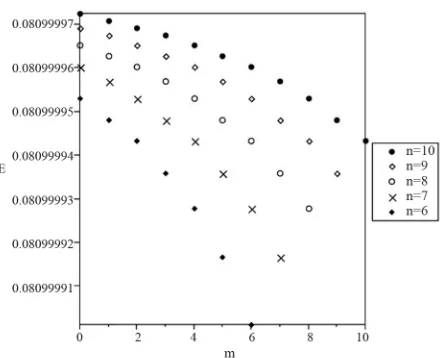
Also, in order to show the effect of spin on the energy spectrum, the obtained energy spectrum of radial part from solving relativistic Schrödinger equation are illus- trated in Figure 1 and Figure 2 as function of quantum numbers n and m.
We may also derive the eigen function of the angular part of the relativistic Schrödinger equation similar to the solution of the radial part. The angular Equation (7) can be further separated by substituting,
,
Θ
ΦY
Table 1. Radial wave function and energy spectrum. Here n and m are the quantum numbers and
ρC
ρ2 ρ 1
. e d
we
assume α 1,β2.
n m Rn m, En m,
1 0 2 eC
1 2 2 2 0 2 1 3
m c
1 1 2C12e
1 2 2 2 0 1 2
m c
2 0 2 2C1 e
1 2 2 2 0 2 1 7
m c
2 1 2C1221 e
1 2 2 2 0 2 1 5
m c
2 2 2 eC
1 2 2 2 0 2 1 3
m c
3 0 3
8 2 24 4 e
6 C 1 2 2 2 0 2 1 11
m c
3 1 2 eC 12
2241 e
1 2 2 2 0 2 1 9
m c
3 2 2 2 1C e
1 2 2 2 0 2 1 7
m c
3 3 2C12e
1 2 2 2 0 2 1 5
m c
4 0 4
3 6 2 9 3 e
3C 1 2 2 2 0 2 1 15
m c
4 1 2 12
4 3 18 2 18 3 e
3 C 1 2 2 2 0 2 1 13
m c
4 2 2
2 2 6 3 e
3C 1 2 2 2 0 2 1 11
m c
4 3
1 2
2 2 3 e
3C 1 2 2 2 0 2 1 9
m c
4 4 4 e
6C 1 2 2 2 0 2 1 7
m c
[image:3.595.308.538.130.726.2]Figure 2. Energy spectrum for n6,,10. We take Φ
as follow,
1 ei2π
m
(23)
So for azimuthal part we have,
2
2 2 2
dΘ
1 d
sin
sin d d
2
Γ Θ 0
sin
S
L S
(24)
where equal to square of quantum number m. The L·Sterm in Equation (24) point to the spin-orbit interact- tion energy. This term simply consider as a perturbation to the final solution, so we ignore it. Here we define a
new constant parameter,
2 2 Γ,
S so the Equation
(24) is rewritten by following expression,
2Θ cot Θ 0
sin
(25)
By introducing a new variable xcos , one can re- write Equation (25) as,
2
2
1 2
1
x x x x x
x
0 (26)
Now we consider wave function as,
x v x w x (27)
Thus the Equation (26) will become,
2 2
2
2
1 2 1 2
1 2
1
w x
x v x x x v x w x
w x w x
x x v x
w x w x x
In order to obtain the wave function Θ
x , we modi-fy this equation with the associated Jacobi differential equation. Here for the real parameters , 1, this equation corresponding ,
, n m
P in the interval x
1,1
is introduced as [24],
2 , ,
, ,
2
, ,
1 2
1
1
0
n m n m
n m
x P x x P
m m x
n n
x
P x
x
(29)
where, the indices n and m are non-negative integers with
0 m n and for m = 0 Equation (29) converts to the differential equation corresponding to the Jacobi Po- lynomials.
After the modification of Equations (28) and (29), in first step one can obtain w x
as,
2d d
2 1 2 1
e .
x x
x
w x C
2
x
x (30)
We conclude that the function in Equation (27) is corresponding to the associated Jacobi function
v x
, , n mP x
as solution of the Equation (29) which has the following Rodriguez representation,
, ,
,
2
,
1 1
d 1 1
d
n m
n m m m
n m
n n
a P x
x x
x x x
2
(31)
Here an m,
,
nm
is the normalization coefficient which for is given by,
, ,
1 1
,
1 1 1
2
n m m
n
a
n m
C
n m n n
(32) In which C
,
is an arbitrary real constant inde-pendent of n and m. Therefore we have following rela- tion for Θ
x ,
2 2
d d
2 1 2 1 ,
, ,
Θ e .
x x x
x x
n m x C Pn m
x (33)
Finally, according to the Equations (23) and (29) the angular wave function is given by,
2 2
d d
2 2
i 1 1 ,
, , e e , c
2π
x x x
m x x
n m n m
C
Y P
os
0
(28) (34)
4. Factorization Method to Wave Equations
In recent years supersymmetry and shape invariance in quantum mechanics have undergone a spectacular deve- lopment. The concepts of shape invariance are developed in several branches of physics, such as atomi, nuclear and mathematical physics as well as quantum optics. Super- symmetry in quantum mechanics is based upon the fac- torization method in the framework of shape invariance. Factorization method goes back to Darboux, but was developed by Schrödinger in order to apply it to quantum mechanics [25,26]. There is a discussion of the factoriza- tion method in the review article of Infield and Hull [27], where they have been shown a large variety of the se- cond-order differential equation with different boundary conditions set in six different types of factorizations. If a quantum mechanics problem admit context of super- symmetry, one able to factorize the Hamiltonian of quan- tum states in terms of a multiplication of the first-order differential operators as the shape invariance equation. In this approach, the Hamiltonians decomposed once in successive multiplication of lowering and raising opera- tors, in such a way that the corresponding quantum states of successive levels are their Eigen states of them. These Hamiltonian are called partner and supersymmetric of each other.
In fact, three separate subject, i.e. the factorization me- thod, the supersymmetry in the quantum mechanics and the shape invariance, nowadays converged at a point. The idea of supersymmetry in the context of quantum mechanics was first study by Nicolai and Witten and la- ter by Cooper and Freedman et al. [28-30]. Recently, Gen- denshtein put forward the concept of shape invariance in the context of the supersymmetric quantum mechanics [31]. As yet, according to the factorization method, many studies on the one-dimensional shape invariance poten- tial in the framework of the supersymmetric quantum mechanics have been carried out [32-38]. One of the most well-known one-dimension quantum mechanical systems is the quantum harmonic oscillator [39]. There are other solvable systems with, say, a Morse potential, Scarf po- tential, Eckart potential, and many others [40-42]. These solvable potentials have established a tight connection with the pioneering work of Infield and Hull on factori- zation and algebraic solution of bound state problems. It should be noted that most of the solvable potentials are shape invariance. On this basis, the one dimension part- ner Hamiltonian is connected by supersymmetry trans- formations. The spectra of two partner Hamiltonians are identical, expect for the ground state. Supersymmetry played important role in analyzing of the quantum me- chanical systems, since it can consider remarkable prop- erties including degeneracy structure of the energy spec-
trum, the relations among the energy spectra of the vari-ous Hamiltonians, derivation of algebraic solutions and etc. In previous section, we determine the radial and an-gular wave functions of relativistic Hydrogen atom. In this section we apply the factorization method to radial and angular parts of Relativistic Schrödinger wave equa-tion. In the first step, we consider the radial part of wave equation obtained in previous section. As mentioned in refs [43,44], one can factorize the associated Laguerre differential equation as the following shape invariance equations with respect to the parameters n and m,
,
,
, , , , ,
n m n m n m n m n m
A r A r L r B L r
,
,, , 1, , 1, ( )
n m n m n m n m n m
A r A r L r B L r (35)
where
,
n m
B nm n (36)
and its associated differential operators are,
,d
d 2
n m
m
A r r r n
r
,d
d 2
n m
m
A r r n
r
(37)
We note that the shape invariance Equations (35) can also be written as the lowering and raising relations,
, ,
, 1, , ,
, ,
, , , 1,
n m n m n m n m
n m n m n m n m
A r r L r B L r A r L r B L r
(38)
Therefore, we obtain the raising and lowering opera-tors for the radial part of the relativistic Hydrogen atom. Next we apply factorization method to the angular part of the Relativistic Schrödinger wave equation. The shape invariance equations of the associated Jacobi differential equation respect to the parameters n and m given by [45,46],
, ,
, , , , ,
,
, , 1, , 1, ( )
n m n m n m n m n m
n m n m n m n m n m
,
A r A r P r C P r A r A r P r C P r
(39)
where
, 2
4
2
n m
n m n n n m C
n
(40)
Therefore raising and lowering operators can be evalu- ated as,
2 ,
2 ,
d 1
d 2
d 1
d 2
n m
n m
n m
A x n x
x n
n m
A x nx
x n
Also in the case of the shape invariance respect to m we have,
, ,
, , ,
,
, 1 , , 1
m m n m n m n m
m m n m n m n m
,
A x A x P x D P x
A x A x P x D P x
(42)
where
, 1
n m
D n m n m
(43)and,
2
2 1 d
1
d 1
m
m x A x x
x x
2
2 d
1
d 1
m
m x A x x
x x
(44)
Note that the shape invariance Equations (39) contain the indices
n m,
and also
n1,m
m
and the shape in- variance Equations (42) contain
n,
n efactorized Equations (39) together describe shape inva- riance with respect to n and also Equations (42) de- scribe shape invariance with respect to m. One can easily rewrite shape invariance Equations (39) and (42) as the laddering relations with respect to the indices n and m respectively,
and 1,m
. Th
, ,
, 1, , ,
, ,
, , , 1,
n m n m n m n m
n m n m n m n m
A x P x C P x
A x P x C P x
(45)
and,
, ,
, 1 , ,
,
, , ,
m n m n m n m
m n m n m n m
, 1
A x P x D P x A x P x D P x
(46)
The general algebra covered this example completed by these raisingwors of radial part make Hr algebra and
the raising andlowering operators of angular part make
H. Therefore we obtain following algebra,
r
HH H (47)
5. Conclusions
In this study, we successfully introduce spin in Schrö- dinger equation. The modification between reformed ra- dial part of this equation for Hydrogen atom and the as- sociated Laguerre differential equation, lead us to derive the exact bound states and corresponding radial wave functions.
Also by applying the factorization method we deter- mine the lowering and raising operators which generate the shape invariance relation of Laguerre differential equation. In similar case, for angular wave functions of Hydrogen atom, the modification between reformed an- gular part of Schrödinger equation and the associated
Jacobi differential equation, give us the exact angular wave functions. The resulting energy levels of Hydrogen atom in this theory are exactly match the results obtained using relativistic Dirac equation.
REFERENCES
[1] W. Greiner, “Quantum Mechanics,” 3rd Edition, Springer- Verlag, Berlin, 1994.
[2] I. T. Todorov, “Quasipotential Equation Corresponding to the Relativistic Eikonal Approximation,” Physical Review D, Vol. 3, 1971, pp. 2351-2356.
doi:10.1103/PhysRevD.3.2351
[3] E. Brezin, C. Itzykson and J. Zinn-Justin, “Relativistic Bal- mer Formula Including Recoil Effects,” Physical Rview D,
Vol. 1, No. 8, 1970, pp. 2349-2355. doi:10.1103/PhysRevD.1.2349.
[4] C. Itzykson and J. B. Zuber, “Quantum Field Theory,” Mc- Graw-Hill, New York, 1985.
[5] E. Fermi and C. N. Yang, “A Relativistic Equation for Bound-State Problems,” Physical Review, Vol. 84, No. 6,
1951, pp. 1232-1242. doi:10.1103/PhysRev.84.1232 [6] E. E. Salpeter and H. A. Bethe, “Are Mesons Elementary
Particles?” Physical Review, Vol. 76, No. 12, 1949, pp.
1739-1743. doi:10.1103/PhysRev.76.1739
[7] G. Breit, “Dirac’s Equation and the Spin-Spin Interac- tions of Two Electrons,” Physical Review, Vol. 39, No. 4,
1932, pp. 616-624. doi:10.1103/PhysRev.39.616
[8] G. D. Tsibidis, “Quark-Antiquark Bound States and the Breit Equation,” Acta Physica Polonica B, Vol. 35, No.
10, 2004, pp. 2329-2365.
[9] R. J. Duffin, “On the Characteristic Matrices of Covariant Systems,” Physical Review, Vol. 54, No. 12, 1939, p.
1114. doi:10.1103/PhysRev.54.1114
[10] J. T. Lunardi, L. A. Manzoni and B. M. Pimentel,“Duf- fin-Kemmer-Petiau Theory in the Causal Approa,” Inter-
national Journal of Modern Physics A, Vol. 17, No. 2,
2002, p. 205. doi:10.1142/S0217751X02005682
[11] I. Boztosun, M. Karakus, F. Yasuk and A. Durmus, “Asy- mptotic Iteration Method Solutions to the Relativistic Du- ffin-Kemmer-Petiau Equation,” Journal of Mathematical
Physics, Vol. 47, No. 6, 2006, Article ID: 062301.
doi:10.1063/1.2203429
[12] Y. Nedjadi and R. C. Barrett, “The Duffin-Kemmer-Pe- tiau Oscillator,” Journal of Physics A: Mathematical and
General, Vol. 27, No. 12, 1994, p. 4301.
doi:10.1088/0305-4470/27/12/033
[13] Y. Nedjadi and R. C. Barrett, “Solution of the Central Field Problem for a Duffin-Kemmer-Petiau Vector Bo- son,” Journal of Mathematical Physics, Vol. 35, No. 9,
1994, pp. 4517-4533. doi:10.1063/1.530801
[14] Y. Nedjadi and R. C. Barrett, “On the Properties of the Duffin-Kemmer-Petiau Equation,” Journal of Physics G:
Nuclear and Particle Physics, Vol. 19, No. 1, 1993, pp.
87-98. doi:10.1088/0954-3899/19/1/006
Vol. 338, No. 2, 2005, pp. 97-107. doi:10.1016/j.physleta.2005.02.029
[16] V. Y. Fainberg and B. M. Pimentel, “Duffin-Kemmer- Petiau and Klein-Gordon-Fock Equations for Electroma- gnetic, Yang-Mills and External Gravitational Field In- teractions: Proof of Equivalence,” Physics Letters A, Vol.
271, No. 1-2, 2000, pp. 16-25. doi:10.1016/S0375-9601(00)00330-3
[17] J. T. Lunardi, P. M. Pimental and R. G. Teixeiri, “Re-marks on Duffin-Kemmer-Petiau Theory and Gauge Inva- riance,” Physics Letters A, Vol. 268, No. 10, 2000, pp.
165-173. doi:10.1016/S0375-9601(00)00163-8
[18] L. Chetouani, M. Merad and T. Boudjedaa, “Solution of Duffin-Kemmer-Petiau Equation for the Step Potential,”
International Journal of Theoretical Physics, Vol. 43, No.
4, 2004, pp. 1147-1159.
doi:10.1023/B:IJTP.0000048606.29712.13
[19] A. Boumali, “Particule de Spin 0 dans un Potentiel d’A- haronov-Bohm,” Canadian Journal of Physics, Vol. 82,
No. 1, 2004, pp. 67-74. doi:10.1139/p03-112
[20] D. A. Kulikov, R. S. Tutik and A. P. Yaroshenko “An Al- ternative Model for the Duffin-Kemmer-Petiau Oscilla- tor,” Modern Physics Letters A, Vol. 20, No. 1, 2005, pp.
43-49. doi:10.1142/S0217732305016324
[21] N. Ogawa, “Quantum Mechanical Embedding of Spin- ning Particle and Induced Spin-Connection,” Modern
Physics Letters A, Vol. 12, No. 21, 1997, pp. 1583-1588.
doi:10.1142/S0217732397001618
[22] H. Koura and M. Yamada, “Single-Particle Potentials for Spherical Nuclei,” Nuclear Physics A, Vol. 671, No. 1-4,
2000, pp. 96-118. doi:10.1016/S0375-9474(99)00428-5 [23] J. Sadeghi “Superalgebras for Three Interacting Particles
in an External Magnetic Field,” European Physical Jour-
nal B, Vol. 50, No. 3, 2006, pp. 453-457.
doi:10.1140/epjb/e2006-00150-9
[24] A. F. Nikiforov and V. B. Uvarov, “Special Functions of Mathematical Physics,” Birkhauser, Basle, 1988.
[25] E. Schrödinger, “A Method of Determining Quantum-Me- chanical Eigenvalues and Eigenfunctions,” Proceedings
of the Royal Irish Academy, Vol. 46A, 1940, pp. 9-16.
[26] E. Schrödinger, “The Factorization of the Hypergeometric Equation,” Proceedings of the Royal Irish Academy, Vol.
47A, 1941, pp. 53-54.
[27] L. Infeld and T. D. Hull, “The Factorization Method,” Re-
views of Modern Physics, Vol. 23, No.1, 1951, pp. 21-68.
doi:10.1103/RevModPhys.23.21.
[28] H. Nicolai, “Supersymmetry and Spin Systems,” Journal
of Physics A, Vol. 9, No. 9, 1976, p. 1497.
doi:10.1088/0305-4470/9/9/010
[29] E. Witten, “Gauge Theories, Vertex Models, and Quan- tum Groups,” Nuclear Physics B, Vol. 380, No. 2-3, 1990,
pp. 285-346.
[30] F. Cooper and B. Freedman, “Aspects of Supersymmetric Quantum Mechanics,” Annals of Physics, Vol.146, No. 2,
1983, pp. 262-288. doi:10.1016/0003-4916(83)90034-9 [31] L. E. Gendenshtein, “Derivation of Exact Spectra of the
Schrödinger Equation by Means of Supper Symmetry,”
Letters to Jounal of Experimental and Theoretical Phy- sics, Vol. 38, 1983, pp. 356-359.
[32] C. X. Chuan, “Exactly solvable potentials and the concept of shape invariance,” Journal of Physics A, Vol. 24, No.
19, 2006, p. L1165. doi:10.1088/0305-4470/24/19/008 [33] F. Cooper, A. Khare and U. Sukhatme, “Supersymmetry
and Quantum Mechanics,” Physics Reports, Vol. 251, No.
5-6, 1995, pp. 267-385.
doi:10.1016/0370-1573(94)00080-M
[34] A. Balantekin, “Algebraic Approach to Shape Invari- ance,” Physical Review A, Vol.57, No. 6, 1998, pp. 4188-
4191. doi:10.1103/PhysRevA.57.4188
[35] A. Balantekin, M. A. C. Ribeiro and A. N. F. Aleixo, “Al- gebraic Nature of Shape-Invariant and Self-Similar Po- tentials,” Journal of Physics A: Mathematical and Gene- ral, Vol. 32, No. 15, 1999, pp. 2785-2790.
doi:10.1088/0305-4470/32/15/007
[36] J. F. Carinena and A. Ramos, “The Partnership of Poten- tials in Quantum Mechanics and Shape Invariance,” Mo-
dern Physics Letters A, Vol. 15, No. 16, 2000, p. 1079.
doi:10.1142/S0217732300001249
[37] H. Aoyama, M. Sato and T. Tanaka, “N-Fold Supersym-
metry in Quantum Mechanics: General Formalism,” Nu-
clear Physics B, Vol. 619, No. 1-3, 2001, pp. 105-127.
doi:10.1016/S0550-3213(01)00516-8
[38] S. W. Qian, B. W. Huang and Z. Y. Gu, “Supersymmetry and Shape Invariance of the Effective Screened Poten- tial,” New Journal of Physics, Vol. 4, 2002, pp. 13.1-13.6.
doi:10.1088/1367-2630/4/1/313
[39] L. Landau and E. M. Lifshitz, “Quantum Mechanics,” Perg- mon, Oxford, 1979.
[40] M. Morse, “Diatomic Molecules According to the Wave Mechanics. Ⅱ. Vibrational Levels,” Physical Review, Vol. 34, No. 1, 1929, pp. 57-64. doi:10.1103/PhysRev.34.57 [41] C. Eckart, “The Penetration of a Potential Barrier by Elec-
trons,”Physical Review, Vol. 35, No. 11, 1930, pp. 1303-
1309. doi:10.1103/PhysRev.35.1303
[42] V. Bargmann,“On the Connection between Phase Shifts and Scattering Potential,” Reviews of Modern Physics,
Vol. 21, No. 3, 1949, pp. 488-493. doi:10.1103/RevModPhys.21.488
[43] J. Sadeghi, “Factorization Method and Solution of the Non-Central Modified Kreutzer Potential,” Acta Physica
Polonica A, Vol. 112, No. 1, 2007, pp. 23-28.
[44] M. A. Jafarizadeh and H. Fakhri, “The Embedding of Pa- rasupersymmetry and Dynamical Symmetry intoGL(2, c)
Group,” Annals of Physics, Vol. 266, No. 1, 1998, pp. 178-
206. doi:10.1006/aphy.1998.5788
[45] M. A. Jafarizadeh and H. Fakhri, “Supersymmetry and Shape Invariance in Differential Equations of Mathema- tical Physic,” Physics Letters A, Vol. 230, No. 3-4, 1997,
pp. 164-170. doi:10.1016/S0375-9601(97)00161-8 [46] H. Fakhri and J. Sadeghi, “Supersymmetry Approaches to
the Bound States of the Generalized Woods-Saxon Poten- tial,” Modern Physics Letters A, Vol. 19, No. 8, 2004, p.