Isomorphic Strategy Spaces in Game Theory

Isomorphic Strategy Spaces in Game

Theory

Gagen, Michael

10 April 2013

Online at

https://mpra.ub.uni-muenchen.de/46176/

Isomorphic Strategy Spaces in Game Theory

Michael J. Gagen

Email: mjgagen at gmail.com

URL: http://www.millitangent.org/

Copyright c_⃝Michael J. Gagen 2013.

All rights reserved. No part of this book may be reproduced in any form by any elec-tronic or mechanical means (including photocopying, recording, or information storage and retrieval) without permission in writing from the author.

Contents

Contents . . . iii

List of Figures . . . vi

List of Tables . . . ix

Preface . . . xi

0.1 Acknowledgments . . . xi

1 Strong isomorphisms in strategy spaces 1 1.1 Introduction . . . 1

1.1.1 Irreducible complexity of strategic optimization . . . 1

1.1.2 Strategy spaces of game theory . . . 2

1.1.3 Isomorphic probability spaces . . . 2

1.1.4 Isomorphism choice alters optimization outcomes . . . 3

1.1.5 Mismatch between probability and game theory . . . 4

1.2 Optimization and isomorphic probability spaces . . . 5

1.2.1 Isomorphic dice . . . 5

1.2.2 Alternate coin probability spaces . . . 10

1.2.3 Joint probability space optimization . . . 14

1.2.4 Entropy maximization . . . 18

1.2.5 Continuous bivariate Normal spaces . . . 19

1.2.6 Quantum probability spaces . . . 21

1.2.7 Perfect correlation reduces dimensionality . . . 21

1.2.8 Example isomorphic functions . . . 23

1.3 Isomorphisms and Optimization . . . 27

1.3.1 Isomorphism constraints alter geometry . . . 27

1.4 Discussion . . . 29

1.5 Appendix: Correlation and mutual information . . . 31

1.5.1 Nonlinear dependencies and correlation . . . 31

1.5.2 Mutual Information . . . 32

2 Isomorphisms in Strategy Spaces 35 2.1 Introduction . . . 35

2.1.1 Mixed strategy probability measure spaces . . . 35

2.2 Mixed and behavioural strategy spaces . . . 37

2.2.1 Mixed strategy space_PM . . . 37

2.2.2 Behavioural strategy space _PB . . . 39

2.2.3 Isomorphic Mixed and Behavioural Spaces . . . 40

2.3 Discussion . . . 42

3 A simple decision tree optimization 43 3.1 Optimizing simple decision trees . . . 43

3.1.1 Non-polylinear payoff functions . . . 43

3.1.2 Polylinear payoff functions . . . 44

4 A simple two-player-two-stage optimization 49 4.1 Optimizing a multistage game tree . . . 49

4.1.1 Unconstrained mixed space _PM . . . 49

4.1.2 Unconstrained behavioural space _PB . . . 50

4.1.3 Constrained behavioural space _PB|_ρxy=ρ . . . 51

4.1.4 Strategic analysis difficulties . . . 52

4.1.5 More general constrained analysis . . . 53

4.2 Backwards induction and isomorphism constraints . . . 58

4.3 Optimizing over multiple joint probability spaces . . . 61

4.3.1 Rational game play: A story . . . 62

4.4 Discussion . . . 68

5 Correlated Equilibria 71 5.1 Introduction . . . 71

5.2 Correlated equilibria . . . 71

6 The chain store paradox 77 6.1 Introduction . . . 77

6.2 The chain store paradox . . . 79

6.2.1 Unconstrained behaviour strategy spaces . . . 79

6.2.2 Isomorphically correlated space _PX B × PBY|q=1 . . . 81

6.2.3 The functionally anti-correlated space: _PX B × PBY|q=0 . . . 82

6.2.4 Expected payoff comparison across multiple probability spaces . . 82

7 The trust game 85 7.1 Introduction . . . 85

7.2 A simplified trust game . . . 85

7.2.1 Unconstrained behaviour strategy spaces . . . 86

7.2.2 The isomorphically correlated space _PX B × PBY|y=¯y . . . 87

CONTENTS v

8 The ultimatum game 91

8.1 Introduction . . . 91

8.2 The Ultimatum game . . . 92

8.2.1 The isomorphically unconstrained space: _PX B × PBY . . . 93

8.2.2 An isomorphically constrained space: _PX B × PBY|y=¯y . . . 94

8.2.3 Payoff comparison across probability spaces . . . 96

8.2.4 An indicative solution reflecting symmetries . . . 96

8.3 Discussion . . . 96

9 The public goods game 99 9.1 Introduction . . . 99

9.2 A simplified public goods game . . . 99

9.2.1 Unconstrained behavioural strategy spaces: _PX B × PBY . . . 101

9.2.2 Isomorphically anti-correlated space _PX B|x2=1−y1 × P Y B|y2=1−x1 . . . 103

9.2.3 Anti-correlated and independent space: _PX B|x2=1−y1 × P Y B . . . 104

9.2.4 Expected payoff comparison . . . 107

10 The centipede game 109 10.1 Introduction . . . 109

10.2 The centipede game . . . 110

10.2.1 The unconstrained space_PX B × PBY . . . 111

10.2.2 Isomorphically constrained spaces . . . 112

10.2.3 The space _PX B|x2=y1,x3=y2 × P Y B|y1=x1,y2=x2,y3=x3 . . . 113

10.2.4 The space _PX B|x2=y1,x3=y2 × P Y B|y2=x2,y3=x3 . . . 114

10.2.5 Expected payoff comparison across multiple probability spaces . . 115

11 The Iterated Prisoner’s Dilemma 117 11.1 Introduction . . . 117

11.2 The finite Iterated Prisoner’s Dilemma . . . 117

11.3 The N = 1 stage Prisoner’s dilemma . . . 120

11.4 The N = 2 stage prisoner’s dilemma . . . 121

11.4.1 The unconstrained space_PX B × PBY . . . 121

11.4.2 Alternate isomorphic probability spaces . . . 123

11.4.3 N = 2 stage: Independent versus Markovian strategies . . . 124

11.4.4 N = 2 stage: Independent versus All Defect strategies . . . 126

11.4.5 N = 2 stage: Independent versus Tit-For-Tat strategies . . . 127

11.4.6 N = 2 stage: Markovian versus Markovian strategies . . . 128

11.4.7 N = 2 stage: Markovian versus All Defect strategies . . . 129

11.4.8 N = 2 stage: Markovian verses Tit-For-Tat strategies . . . 130

11.4.9 N = 2 stage: Comparing payoffs . . . 131

11.4.10N = 2 stage: Extended isomorphic constraints . . . 133

11.5.1 N _≥2: Independent strategies . . . 136

11.5.2 N _≥2: Markovian versus Independent spaces . . . 137

11.5.3 N _≥2: Markovian versus Markovian strategies . . . 139

11.5.4 N _≥2: Comparing payoffs . . . 140

11.5.5 N _≥2: Endgame analysis . . . 141

12 Conclusion 147 12.1 The foundations of strategic analysis . . . 147

List of Figures

1.1 Three alternate dice . . . 6

1.2 The target strategy spaces for alternate dice . . . 9

1.3 A four-sided square probability space . . . 14

1.4 Maximizing joint entropy . . . 19

1.5 Affine transforms of correlated variable . . . 22

1.6 Schematic representation of target strategy space . . . 26

1.7 Correlation constraints in the strategy space . . . 28

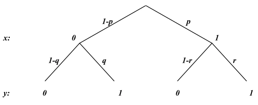
2.1 A simple decision tree . . . 37

3.1 A non-strategic decision tree . . . 44

3.2 A correlated decision tree . . . 45

3.3 An independent decision tree . . . 45

3.4 An anti-correlated decision tree . . . 46

4.1 A two-player strategic game . . . 50

4.2 Alternate probability space gradients . . . 53

4.3 Decision trees, payoffs and equilibria for a simple game . . . 56

4.4 Rational play using the conventional probability space . . . 63

4.5 Rational play using a correlated probability space . . . 64

4.6 Rational play using a hidden probability space . . . 66

4.7 Rational play using alternate probability spaces . . . 67

5.1 Correlated equilibria: An example . . . 72

5.2 Correlated equilibria: Nash equilibria without communication . . . 73

5.3 Correlated equilibria: Communication alters decision tree . . . 74

5.4 Correlated equilibria: Flow diagram . . . 76

6.1 The chain store paradox . . . 79

6.2 Nash equilibria for the chain store paradox . . . 80

7.1 The trust game . . . 86

7.2 Isomorphically correlated choices in the trust game . . . 87

8.1 The Ultimatum game: Conventional analysis . . . 92

8.2 The Ultimatum game: Isomorphically constrained strategies . . . 95

9.1 The public goods game . . . 100

9.2 The public goods game: Anti-correlated choices . . . 103

9.3 The public goods game: Correlated and independent strategies . . . 105

10.1 The centipede game . . . 109

10.2 The centipede game: Isomorphic probability spaces and decision trees . . 116

11.1 A two stage iterated prisoner’s dilemma . . . 118

11.2 Independent and Markovian strategies . . . 124

11.3 Independent and mutual defection strategies . . . 126

11.4 Independent and Tit-For-Tat strategies . . . 127

11.5 Dual Markovian strategies . . . 128

11.6 Markovian and mutual defection strategies . . . 129

11.7 Markovian and Tit-For-Tat strategies . . . 130

List of Tables

2.1 Mixed and Behavioural Spaces and Isomorphic Constraints . . . 41

11.1 The prisoner’s dilemma: Extended payoff table . . . 134 11.2 The prisoner’s dilemma: Alternate isomorphic equilibria . . . 144

xi

Preface

This book summarizes ongoing research introducing probability space isomorphic map-pings into the strategy spaces of game theory.

This approach is motivated by discrepancies between probability theory and game theory when applied to the same strategic situation. In particular, probability theory and game theory can disagree on calculated values of the Fisher information, the log likelihood function, entropy gradients, the rank and Jacobian of variable transforms, and even the dimensionality and volume of the underlying probability parameter spaces. These differences arise as probability theory employs structure preserving isomorphic mappings when constructing strategy spaces to analyze games. In contrast, game theory uses weaker mappings which change some of the properties of the underlying probability distributions within the mixed strategy space. Here, we explore how using strong isomorphic mappings to define game strategy spaces can alter rational outcomes in simple games .

Specific example games considered are the chain store paradox, the trust game, the ultimatum game, the public goods game, the centipede game, and the iterated prisoner’s dilemma. In general, our approach provides rational outcomes which are consistent with observed human play and might thereby resolve some of the paradoxes of game theory.

0.1

Acknowledgments

Chapter 1

Strong isomorphisms in strategy

spaces

1.1

Introduction

1.1.1

Irreducible complexity of strategic optimization

The essential problem of economics and the rational for game theory was first posed by von Neumann and Morgenstern [1]. They described the fundamental economic opti-mization problem by contrasting the non-strategic single player case with the strategic multi-player situation. In particular, they stated the non-strategic case is “an economy which is represented by the ‘Robinson Crusoe’ model, that is an economy of an isolated single person, or otherwise organized under a single will.” In this economy, “Crusoe faces an ordinary maximization problem, the difficulties of which are of a purely technical—and not conceptual—nature”. This non-strategic case was contrasted with a strategic “social exchange economy [where] the result for each one will depend in general not merely upon his own actions but on those of the others as well. . . . This kind of problem is nowhere dealt with in classical mathematics. . . . this is no ordinary maximization problem, no problem of the calculus of variations, of functional analysis, etc” [1].

Thus, von Neumann and Morgenstern essentially claimed that strategic optimization problems were irreducibly more complex than non-strategic optimization problems. And yet, after learning a few new techniques, the solution of strategic games turns out to be not significantly more complex than the solution of non-strategic decision trees—larger and more difficult certainly, but not irreducibly more complex. In this work, we claim that the proposed solution to strategic analysis is incomplete. We will argue that strategic optimization is indeed irreducibly more complex than non-strategic optimization, and this irreducible complexity is missing from current formulations of strategic optimization.

We will look for this missing irreducible complexity by applying probability theory and game theory to the same strategic situation, and examining any differences that arise. We will show that when applied to the same strategic game, probability theory

and game theory can disagree on calculated values of the Fisher information, the log likelihood and entropy gradients, the rank and Jacobian of variable transforms, and even the dimensionality and volume of the underlying probability parameter spaces. These differences arise as probability theory employs structure preserving, isomorphic mappings when constructing a mixed strategy space to analyze games. In contrast, game theory uses weaker mappings which change some of the properties of the underlying probability distributions within the mixed strategy space. We will explore how using strong iso-morphic mappings to define mixed strategy spaces can alter rational outcomes in simple games, and might resolve some of the paradoxes of game theory.

1.1.2

Strategy spaces of game theory

One possibly fruitful way to gain insight into the paradoxes of game theory is to show that probability theory and game theory analyze simple games differently. It would be expected of course that these two well developed fields should always produce consistent results. However, we will show in this paper that probability theory and game theory can produce contradictory results when applied to even simple games. These differences arise as these two fields construct mixed strategy spaces differently.

The mixed strategy space of game theory is constructed, according to von Neumann and Morgenstern, by first making a listing of every possible combination of moves that players might make and of all possible information states that players might possess. This complete embodiment of information then allows every move combination to be mapped into a probability simplex whereby each player’s mixed strategy probability parameters belong to “disjoint but exhaustive alternatives, . . . subject to the [usual normalization] conditions . . . and to no others.” [1]. The resulting unconstrained mixed strategy space is then a “complete set” of all possible probability distributions that might describe the moves of a game [1, 2, 3, 4, 5]. Further, the absence of non-normalization constraints ensures “trembles” or “fluctuations” are always present within the mixed strategy space so every possible pure strategy probability distribution is played with non-zero (but possibly infinitesimal) probability [6]. Together, these properties of the mixed strategy space—a complete set of “contained” probability distributions, no additional constraints, and ever present trembles—lead to inconsistencies with probability theory.

1.1.3

Isomorphic probability spaces

1.1. INTRODUCTION 3

spaces are isomorphic if and only if their dimensionality is identical [7]. When the preser-vation of structure is exact, then calculations within either space must give identical results. Conversely, if the degree of structure preservation is less than exact, then dif-ferences can arise between calculations performed in each space. It is thus crucial to examine the fidelity of the “containment” mappings used to construct the mixed spaces of game theory. Probability theory defines isomorphic probability spaces as follows. We give two definitions for completeness, see Refs. [8, 9, 10].

Definition 1: A probability space _P = _{Ω, σ, P_} consists of a set of events Ω, a

sigma-algebra of all subsets of those events σ, and a probability measure defined over

the eventsP. Two probability spaces _P =_{Ω, σ, P_} and _P′ _={Ω′_{, σ}′_{, P}′_{} are said to be}

strictly isomorphic if there is a bijective (1-to-1 and onto) mapf : Ω_→Ω′ _{which exactly}

preserves assigned probabilities, so for all e _∈ Ω we have P(e) = P′_{[f(e)]. A slight}

weakening of this definition defines an isomorphism as a bijective mapping f of some

unit probability subset of Ω onto a unit probability subset of Ω′_{. That is, the weakened}

mapping ignores null event subsets of zero probability.

Definition 2: Two probability spaces _P = _{Ω, σ, P_} and _P′ _{= {Ω}′_{, σ}′_{, P}′_{} are}

isomorphic if there are null event sets Ω0 _{∈ Ω and Ω}′0 _{∈ Ω}′ _{and an isomorphism}

f : (Ω₋Ω0_)→(Ω′_−Ω′0_{) between the two measurable spaces (Ω−Ω}0_{, σ) and (Ω}′_−Ω′0_{, σ}′₎

with the added properties that P′_{(F) = P[f}−1_{(F)] forF ∈σ}′ _{and P(G) =P}′_{[f(G)] for}

G_∈σ. In other words, an isomorphism exists if there is an invertible measure-preserving

transformation between the unit probability events in each space, (Ω ₋Ω0_{) ∈ Ω and}

(Ω′_−Ω′0_{)∈ Ω}′_{. This also implies that the null probability event sets of each space are}

mapped to each other.

In particular, we note that strong isomorphisms between source and target probability spaces require they have identical dimensionality and tangent spaces [11].

1.1.4

Isomorphism choice alters optimization outcomes

The mixed strategy space of game theory “contains” different probability distributions many possessing different dimensionality (according to probability theory). Their altered dimensionality within the mixed space can alter those computed outcomes dependent on dimensionality. A simple illustration of this process can make this clear.

A 1-dimensional function f(x) can be embedded within a 2-dimensional function

g(x, y) in two ways: using constraints g(x, y0) = f(x), or limits limy_→y0g(x, y) = f(x).

In either case, many of the properties of the source functionf(x) are preserved, but not

necessarily all of them. In particular, these different methods alter gradient optimization calculations. That is, the gradient is properly calculated when constraints are used,

f′_{(x) = g}′_{(x, y}

0), but not when a limit process is used, f′(x) ̸= limy_→y0∇g(x, y) (where

∇ indicates a gradient operator).

expected payoff functions at different points within a probability space. However, we remind ourselves that every comparison of an expected payoff function over a probability

space is equivalent to evaluating a gradient. Specifically, a function Π(x, y) with

expec-tation _⟨Π(a)_⟩ compared at the points a1 and a2 within a probability space employs the

identity

⟨Π(a2)⟩ − ⟨Π(a1)⟩=∇⟨Π(a)⟩.d21, (1.1)

where the distance vector is d21 = ˆa(a2−a1). This results as all expectations are

poly-linear in each probability parameter.

1.1.5

Mismatch between probability and game theory

In this paper, we will show that exactly the same discrepancies arise when probability theory and game theory are applied to simple probability spaces, and that these discrep-ancies can be significant. It is useful to indicate the magnitude of these discrepdiscrep-ancies here to motivate the paper (with full details given in later sections below). We

con-sider a simple card game with two potentially correlated variables x, y _{∈ {}0,1_} with

joint probability distribution Pxy. In the case where x and y are perfectly correlated,

probability theory (denoted by P) and game theory (denoted by G) respectively assign

different dimensions to both the Fisher information matrix (F) and the gradient of the

log Likelihood function (_∇L), and can disagree on the value of the gradient of the joint

entropy at some points (_∇Exy):

P G

dim(F) 1 3

dim(_∇L) 1 3

|∇Exy| 0 ∞.

(1.2)

These fields also disagree on the probability space gradients of both the normalization

condition (P00 +P11 = 1) and the requirement that the joint entropy equates to the

marginal entropy (Exy−Ex = 0):

P G

∇(P00+P11) 0 ̸= 0

∇(Exy −Ex) 0 ̸= 0.

(1.3)

Should these fields model a change of variable within this game, they further disagree

on the rank of the transform matrix (A), and on the invertibility of the Jacobian matrix

(J):

P G

Rank(A) 1 2

J Singular Invertible.

1.2. OPTIMIZATION AND ISOMORPHIC PROBABILITY SPACES 5

These fields even disagree on the dimension (d) and volume (V) of the minimal probability

space used to analyze the game:

P G

d 1 3

V 1 1

6.

(1.5)

The differences between game theory and probability theory arise due to the different use of isomorphic mappings to construct mixed strategy spaces.

We now show the necessity for considering isomorphic probability spaces using exam-ples ranging from simple dice games to bivariate normal distributions.

1.2

Optimization and isomorphic probability spaces

In this section, we introduce the need to use isomorphic mappings when embedding probability spaces within mixed spaces.

1.2.1

Isomorphic dice

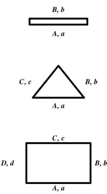
Consider the three alternate dice shown in Fig. 1.1 representing a 2-sided coin, a 3-sided triangle, and a 4-sided square. Faces are labeled with capital letters and the probabilities of each face appearing are labeled with the corresponding small letter. The corresponding probability spaces defined by these die are

Pcoin = _{x_{∈ {}A, B_},_{a, b_}}

Ptriangle = {x∈ {A, B, C},{a, b, c}}

Psquare = _{x_{∈ {}A, B, C, D_},_{a, b, c, d_}}. (1.6)

Here the required sigma-algebras are not listed, and each of these spaces are subject to the usual normalization conditions. For notational convenience we sometimes write

(p1, p2, p3, p4) = (a, b, c, d) and denote the number of sides of each respective die as n ∈

{2,3,4_}. In each respective die space, the gradient operator is

∇=

n₋1

∑

i=1 ˆ

pi

∂ ∂pi

(1.7)

where a hatted variable ˆpi is a unit vector in the indicated direction and we resolve the

normalization constraint via pn = 1−∑ni=1−1pi.

We now wish to optimize a nonlinear function over these spaces, and we choose a function which cannot be optimized using standard approaches in game theory. The chosen function is

A, a

B, b

C , c

D, d

A, a

B, b

C , c

A, a

B, b

Figure 1.1: Three alternate dice with different numbers of sides. A coin with sides A

and B appearing with respective probabilities a and b, a triangle with faces A, B and C occurring with respective probabilities a, band c, and a square die with facesA, B, C and D each occurring with respective probabilities a, b, c and d.

with

V =

∫

spacedv

Ex = −

n

∑

i=1

pilogpi, (1.9)

where V is the volume of each respective probability parameter space and Ex is the

1.2. OPTIMIZATION AND ISOMORPHIC PROBABILITY SPACES 7

As a first pass at optimizing the functionf, we simply maximize f within each

prob-ability space and then compare the optimal outcomes to determine the best achievable

outcome. As is well understood, the entropy of a set ofn events is maximized when those

events are equiprobable giving a maximum entropy of Ex,max = logn. In addition, for

the coin we have

V =

∫ 1

0 da

∫ 1

0 db δa+b=1 =

∫ 1

0 da = 1

Ex = −[alog(a) + (1−a) log(1−a)]

∇Ex = −ˆalog

a

1₋a. (1.10)

For the triangle, the equivalent functions are

V = ∫ 1 0 da ∫ 1 0 db ∫ 1

0 dc δa+b+c=1 =

∫ 1

0 da

∫ 1−a

0 db

= 1

2

Ex = −[alog(a) +blog(b) + (1−a−b) log(1−a−b)]

∇Ex = −aˆlog

a

1₋a₋b −ˆblog

b

1₋a₋b. (1.11)

Finally, for the square, we have

V = ∫ 1 0 da ∫ 1 0 db ∫ 1 0 dc ∫ 1

0 dd δa+b+c+d=1 =

∫ 1

0 da

∫ 1

0 db

∫ 1−a−b

0 dc

= 1

6

Ex = −[alog(a) +blog(b) +clog(c) + (1−a−b−c) log(1−a−b−c)]

∇Ex = −ˆalog

a

1₋a₋b₋c−ˆblog

b

1₋a₋b₋c −cˆlog

c

1₋a₋b₋c. (1.12)

Consequently, the function f takes maximum values in the three probability spaces of

fcoin,max = log 2

ftriangle,max = log 3

4

fsquare,max = log 4

36 . (1.13)

The second method uses isomorphisms to map all of the three incommensurate source spaces into a single target space. We choose our mappings as follows:

Pcoin′ = {x∈ {A, B, C, D},{a, b, c, d}}|(cd)=(00) Ptriangle′ = {x∈ {A, B, C, D},{a, b, c, d}}|d=0

Psquare′ = {x∈ {A, B, C, D},{a, b, c, d}}. (1.14) Here, while all probability spaces share a common event set and probability

distribu-tion, the isomorphic mappings impose constraints on the _P′

coin and Ptriangle′ spaces. The constraints arise from mapping the null sets of zero probability from each source space to the corresponding events of the enlarged target space. The target probability space

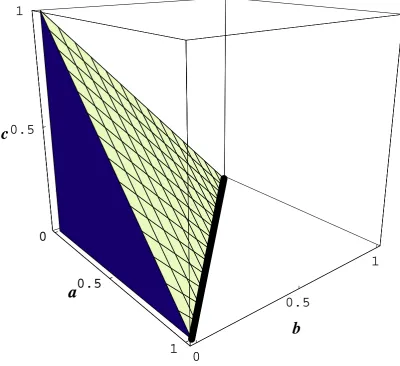
is shown in Fig. 1.2 where the normalization condition d = 1₋a₋b₋c is used. The

points corresponding to the probability spaces of the coin_P′

coin are mapped along the line

a+b = 1 with constraint (c, d) = (0,0). Those points corresponding to the probability

spaces of the triangle _P′

triangle are mapped along the surfacea+b+c= 1 with constraint

d= 0. Finally, the probability spaces corresponding to the square _P′

square fill the volume

a+b+c+d= 1 and are not subject to any other constraint.

The interesting point about the target space is that many points, e.g. (a, b, c, d) =

(1 2,

1

2,0,0), lie in all of the probability spaces of the coin, triangle, and square die and are

only distinguished by which constraints are acting. That is, when this point is subject to

the constraint (cd) = (00), then it corresponds to the probability space_P′

coin (and not to

any other). Conversely, when this same point is subject to an imposed constraint d= 0

then it corresponds to the probability space_P′

triangle. Finally, when no constraints apply then, and only then does this point correspond to the probability space of the square P′

square. This means that it is not the probability values possessed by a point which determines its corresponding probability space but the probability values in combination with the constraints acting at that point.

It is now straightforward to use the isomorphically constrained target space to

max-imize the function f over all embedded probability spaces using standard constrained

optimization techniques. For instance, to optimize f over points corresponding to the

coin and subject to the constraint (c, d) = (0,0) then either simply resolve the constraint

via setting c = d = 0 before the optimization begins, or simply evaluate the gradient

of f at all points (a, b,0,0) in the direction of the unit vector _√1

2(1,−1,0,0) lying along

the line a+b = 1. In more detail, the function f(a, b, c) has a directed gradient in the

direction √1

2(1,−1,0) of

∇f(a, b, c).√1

2(1,−1,0) =V

2_√1

2log

b

a (1.15)

using Eq. 1.12. The rate of change off with respect to the only remaining variablea is

given by

df da =

√

2_∇f.√1

1.2. OPTIMIZATION AND ISOMORPHIC PROBABILITY SPACES 9

0

0.5

1

a

0

0.5

1

b

0.5

1

c

0

0.5

1

a

Figure 1.2: The target space containing points corresponding to the probability spaces

respectively of the coin _P′

coin along the linea+b= 1 with constraint (c, d) = (0,0)(heavy

line), of the triangle_P′

triangle along the surface a+b+c= 1 with constraint d= 0 (hashed

surface), and of the square _P′

square filling the volume a+b+c+d = 1 (filled polygon).

Note that points such as (a, b, c) = (0.5,0.5,0) correspond to all three probability spaces and are only distinguished by which constraints are acting.

Altogether, at points where (a, b, c) = (a,1₋a,0) this gives a directed gradient of

df da =V

2_log 1−a

a (1.17)

which is optimized at (a, b, c) = (1₂,1₂,0). An optimization over all three isomorphic

constraints leads to the same outcomes as obtained previously in Eq. 1.13 with the same result. This completes the second optimization analysis and as promised, it is consistent with the results of the first.

spaces of the triangle and of the coin. This allows a square probability space to mimic

a coin probability space by simply taking the limit (c, d) _→(0,0). Similarly, the square

mimics the triangle through the limit d _→ 0. In turn, this means that an optimization

over the space of the square is effectively an optimization over every choice of space within the square. Specifically, game theory discards constraints to model the choice between contained probability spaces. This optimization over the points of the square

has already been completed above. When optimizing the function f over the

uncon-strained points corresponding to the square, the maximum value is f = log(4)/36 at

(a, b, c, d) = (1₄,1₄,1₄,1₄), and according to game theory, this is the best outcome when players have a choice between the coin, the triangle, or the square.

The optimum result obtained by the third optimization method, that used by game theory, conflicts with those found by the previous two methods as commonly used in probability theory. The difference arises as game theory models a choice between proba-bility spaces by making players uncertain about the values of their probaproba-bility parameters within any probability space. Consequently, their probability parameters are always

sub-ject to infinitesimal fluctuations, i.e. c > 0+ _{or d >0}+ _{always. These fluctuations alter}

the dimensions of the space which impacts on the calculation of the volumeV and alters

the calculated gradient of the entropy. Game theory eschews the role of isomorphism con-straints within probability spaces on the grounds that any such concon-straints restrict player uncertainty and hence their ability to choose between different probability spaces. The probability parameter fluctuations mean that players have access to all possible proba-bility dimensions at all times so a single mixed space is the appropriate way to model the choice between contained probability spaces. In contrast, probability theory holds that the choice between probability spaces introduces player uncertainty about which space to use, but specifically does not introduce uncertainty into the parameters within any indi-vidual probability space. As a result, probability theory employs isomorphic constraints to ensure that the properties of each embedded probability space within the mixed space are unchanged.

The upshot is that a game theorist cannot evaluate the Entropy (or uncertainty) gradient of a coin toss while considering alternate die because uncertainty about which dice is used bleeds into the Entropy calculation. However, the probability theorist will distinguish between their uncertainty about which face of the coin will appear and their uncertainty about which dice is being used.

1.2.2

Alternate coin probability spaces

The preceding section has shown the importance of using isomorphism constraints to

preserve the properties of the coin probability space _Pcoin when embedded within larger

1.2. OPTIMIZATION AND ISOMORPHIC PROBABILITY SPACES 11

the physical apparatus and the probability space. We illustrate this now by adopting several different probability spaces for a coin.

In the preceding sections, we have the physical coin as shown in Fig. 1.1 and its corresponding probability space as defined in Eq. 1.6. To reiterate,

Pcoin={x∈ {A, B},{a, b}}. (1.18)

After taking account of the normalization constraint b = 1₋a, the gradient operator in

this space is

∇= ˆa ∂

∂a. (1.19)

If we define a payoff via the random variable Π(A) = 0 and Π(B) = 1, then a gradient

optimization gives

∇⟨Π_⟩ = _∇P(B)

= ₋aˆ (1.20)

indicating that expected payoffs are maximized by settinga = 0 as expected.

There are many very different formulations possible for the probability space of a simple two sided coin, and these are considered to be functionally identical only after the appropriate structure-preserving isomorphisms have been defined. Every alternative in-troduces a different parameterization which alters dimensionality and gradient operators and modifies the optimization algorithm. We illustrate this now.

Our coin could be optimized using a probability measure space _P2

coin involving two

uncorrelated coins, namely

Pcoin2 ={(x, y)∈ {(0,0),(0,1),(1,0),(1,1)},{(1−p)(1−q),(1−p)q, p(1−q), pq}}. (1.21)

An isomorphism can be defined by mapping event A onto the event set (x, y) _∈

{(0,0),(1,1)_} and B onto (x, y)_{∈ {}(0,1),(1,0)_}. In this space, the gradient operator is

∇= ˆp ∂ ∂p + ˆq

∂

∂q (1.22)

and a gradient optimization of the expected payoff gives

∇⟨Π_⟩ = _∇P(B)

= ˆp(1₋2q) + ˆq(1₋2p). (1.23)

This shows that whenq < 1₂ then payoffs are maximized by settingp= 1 and conversely,

when p < 1₂ then payoffs are maximized by setting q = 1.

Alternatively, the binary decision could be optimized using a continuously

param-eterized probability measure space _P3

coin. In this space, the choices A and B might be

determined using a continuously distributed variableu_∈(_−∞,_∞) possessing a normally

distributed probability distribution

P(u) = √1

2πσe

−12 (u−u¯)2

with mean ¯u, standard deviation σ, and variance σ2_{. We introduce a new parameter,p,}

so outcome A occurs with probability

P(A) = √1

2πσ

∫ p

−∞du e −1

2 (u−u¯)2

σ2 , (1.25)

while outcome B occurs with probability

P(B) = √1

2πσ

∫ ∞

p du e

−1 2

(u−u¯)2

σ2 . (1.26)

This space has only one probability parameter pso the gradient operator is

∇= ˆp ∂

∂p, (1.27)

and optimizing the expected payoff gives

∇⟨Π_⟩ = _∇√1

2πσ

∫ ∞

p du e

−1 2

(u−u¯)2

σ2

= _−∇F(p), (1.28)

whereF(p) is the cumulative normal distribution. As the cumulative normal distribution

is monotonically increasing, _∇F(p)>0, so the expected payoff is maximized by setting

p_{→ −∞}giving P(B) = 1 as expected.

For a more extreme alternative, consider a quantum probability measure space _P4

coin

in which event A corresponds to a measurement finding a two-state quantum system

in its ground state, and event B occurs when the measurement finds the system in its

excited state. Writing the quantum system state as

|Ψ_⟩=

    a b   

, (1.29)

where a and b are complex numbers satisfying _|a_|2_+|b|2 _{= 1, then we have P(A) =|a|}2

and P(B) =_|b_|2_{. In this space, the payoff is an operator}

Π =     0 0 0 1   

, (1.30)

giving the expected payoff as

⟨Π_⟩ = _⟨Ψ_|Π_|Ψ_⟩ = _|b_|2

= r2, (1.31)

where in the last line we write b = reiθ _{with real 0}

≤ r _≤ 1 and 0 _≤ θ < 2π. Here,

the expected payoff depends only on the single real variable r so optimization is via the

gradient operator

∇= ˆr ∂

1.2. OPTIMIZATION AND ISOMORPHIC PROBABILITY SPACES 13

giving

∇⟨Π_⟩= 2r. (1.33)

As required, maximization requires setting r= 1, with θ arbitrary.

For a last example, consider a probability space_P5

coinwhich selects a number uin the

Cantor set _C with uniform probability P(u) such that when u _≤ p then event A occurs

while when p < u then event B occurs. The Cantor set _C is interesting as it has an

uncountably infinite number of members and yet has measure zero [13]. In this space, the expected payoff is

⟨Π_⟩ = ∑

u_∈C

P(u)Π(u)

= ∑

u>p_∈C

P(u)

= 1₋C(p), (1.34)

whereC(p) is the cumulative probability distribution termed the Cantor function.

Inter-estingly, the Cantor function is an example of a “Devil’s staircase”, a function which is continuous but not absolutely continuous everywhere, and is differentiable with deriva-tive zero almost everywhere, and which maps the measure zero Cantor set continuously

onto the measure one set [0,1] [13]. As with the normal distribution example above,

the Cantor function is nondecreasing allowing an intuitive maximization of the expected payoff via the gradient operator

∇= ∂

∂p (1.35)

giving

∇⟨Π_⟩=₋dC(p)

dp . (1.36)

As the cumulative normal distribution is nondecreasing, we have dC_dp(p) _≥0 so the expected

payoff is maximized by settingp= 0. This intuitive ansatz suffices for our purposes here.

Lastly, the player is of course, not restricted to using only simple probability mea-sure spaces, and more complicated spaces can be considered. In fact, players will most likely use a pseudo-random number generator consisting of the correlated dynamical in-teractions of some millions (or more) of electronic components in a computer. It is only the correlations of these millions of variables that allows a dimensionality reduction to the few variables required to model the player’s chosen probability space. Isomorphisms underlie the dimensionality reductions of random number generators.

H

00

L

, a

H

01

L

, b

H

10

L

, c

H

11

L

, d

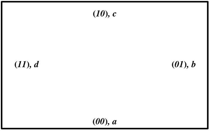
Figure 1.3: A four-sided square probability space where joint variablesxandy take values

(x, y)_{∈ {}(0,0),(0,1),(1,0),(1,1)_} with respective probabilities (a, b, c, d).

1.2.3

Joint probability space optimization

We will briefly now examine isomorphisms between the joint probability spaces of two arbitrarily correlated random variables. In particular, we consider two random variables

x, y as appear on the square dice of Fig. 1.3 with probability space

Psquare = {(x, y)∈ {(0,0),(0,1),(1,0),(1,1)},{a, b, c, d}}. (1.37)

The correlation between the x and y variables is

ρxy = ⟨

xy_{⟩ − ⟨}x_⟩⟨y_⟩ σxσy

= √ ad−bc

(c+d)(a+b)(b+d)(a+c). (1.38)

Here, σx and σy are the respective standard deviations of the xand y variables.

The space _Psquare of course contains many embedded or contained spaces. We will

separately consider the case where x and y are perfectly correlated, and where they are

independent. As noted previously, there are two distinct ways for these spaces to be

contained within _Psquare, namely using isomorphism constraints or using limit processes.

These two ways give the respective definitions for the perfectly correlated case

Pcorr = {(x, y)∈ {(0,0),(0,1),(1,0),(1,1)},{a, b, c, d}}|b=c=0

Pcorr′ = lim

(bc)→(00){(x, y)∈ {(0,0),(0,1),(1,0),(1,1)},{a, b, c, d}} (1.39) and for the independent case

Pind = {(x, y)∈ {(0,0),(0,1),(1,0),(1,1)},{a, b, c, d}}|ad=bc

Pind′ = _adlim

1.2. OPTIMIZATION AND ISOMORPHIC PROBABILITY SPACES 15

Here, all spaces satisfy the normalization constrainta+b+c+d= 1, which we typically

resolve using d = 1₋a₋b ₋c. The gradient operator in the probability space of the

square dice with probability parameters (a, b, c) is

∇= ˆa ∂

∂a + ˆb ∂ ∂b + ˆc

∂

∂c, (1.41)

where a hat indicates a unit vector in the indicated direction. Evaluating any function dependent on a gradient or completing an optimization task using either isomorphic con-straints or limit processes can naturally result in different outcomes as we now illustrate.

Perfectly correlated probability spaces

We first consider the case where the x and y variables are perfectly correlated in the

spaces _Pcorr with isomorphism constraints orPcorr′ using limit processes.

The maximum achievable joint entropy [12] for our two perfectly correlated variables obviously occurs at the point where they are equiprobable. This can be found by evalu-ating the gradient of the joint entropy function

Exy(a, b, c) = −

∑

xy

PxylogPxy (1.42)

= ₋aloga₋blogb₋clogc₋(1₋a₋b₋c) log(1₋a₋b₋c)

giving respective gradients in the _Pcorr and Pcorr′ spaces of

∇Exy|b=c=0 = −ˆalog

( a

1₋a

)

∇Exy = −ˆalog

( a

1₋a₋b₋c

)

−ˆblog

(

b

1₋a₋b₋c

)

−cˆlog

( c

1₋a₋b₋c

)

lim

(bc)→(00)∇Exy = undefined. (1.43)

Equating these gradients to zero locates the maximum at (a, b, c) = (1

2,0,0) in Pcorr and

at (a, b, c) = (1 4,

1 4,

1

4) in Pcorr′ .

The Fisher Information is defined in terms of probability space gradients as the amount of information obtained about a probability parameter from observing any event

[12]. Writing (a, b, c) = (p1, p2, p3), the Fisher Information is a matrix with elements

i, j _{∈ {}1,2,3_} with

Fij =

∑ xy Pxy ( ∂ ∂pi

logPxy

) ( ∂ ∂pj

logPxy

)

. (1.44)

When isomorphically constrained in the space _Pcorr, the Fisher Information is Fij|b=c=0

with the only nonzero term being

F11 = (1−a)

[

ˆ

a ∂

∂a log(1−a)

]2

+a

[

ˆ

a ∂ ∂a loga

]2

= 1

This means that the smaller the Variance the more the information obtained abouta. In

the unconstrained space_P′

corr, the Fisher Information is a very different, 3×3 matrix.

Probability parameter gradients also allow estimation of probability parameters by

locating points where the Log Likelihood function is maximized _∇logL = 0 [12]. This

evaluation takes very different forms in the isomorphically constrained space_Pcorrand the

unconstrained space_P′

corr. The likelihood function estimates probability parameters from

the observation of ntrials with naappearances of event (x, y) = (0,0), nb appearances of

event (x, y) = (0,1), nc appearances of event (x, y) = (1,0), and nd appearances of event

(x, y) = (1,1). We have na+nb+nc+nd=n, giving the Likelihood function

L=f(na, nb, nc, n)anabnbcnc(1−a−b−c)n−na−nb−nc (1.46)

where f(na, nb, nc, n) gives the number of combinations. The optimization proceeds by

evaluating the gradient of the Log Likelihood function. When isomorphically constrained

in the space _Pcorr, the gradient of the Log Likelihood function is

∇logL_|b=c=0 = ˆa

[n

a

a −

n₋na

1₋a

]

, (1.47)

which equated to zero gives the optimal estimate at a = na/n and nb = nc = 0 as

expected. Conversely, when unconstrained in the space _P′

corr, the gradient of the Log

Likelihood function evaluates as

∇logL = ˆa

[n

a

a −

n₋na−nb−nc

1₋a₋b₋c

]

+ ˆb

[n

b

b −

n₋na−nb−nc

1₋a₋b₋c

]

+ˆc

[n

c

c −

n₋na−nb−nc

1₋a₋b₋c

]

. (1.48)

This is obviously a very different result. However, in our case the same estimated

out-comes can be achieved in both spaces. For example, if an observation ofntrials showsna

instances of (x, y) = (0,0) and n₋na instances of (x, y) = (1,1) then both constrained

and unconstrained approaches give the best estimates of the probability parameters of (a, b, c, d) = (na

n,0,0,1− na

n).

Finally, when x and y are perfectly correlated it is necessarily the case that

expecta-tions satisfy _⟨x_{⟩ − ⟨}y_⟩= 0, that variances satisfyV(x)₋V(y) = 0, that the joint entropy

is equal to the entropy of each variable so Exy−Ex = 0, and that finally, the correlation

between these variables satisfiesρxy−1 = 0. In the unconstrained probability spacePcorr′ ,

the expectation, variance, and entropy relations of interest evaluate as

⟨x_{⟩ − ⟨}y_⟩ = c₋b

V(x)₋V(y) = (c₋b)(a₋d) (1.49)

Ex = −[(a+b) log(a+b) + (1−a−b) log(1−a−b)]

Exy = −[aloga+blogb+clogc+ (1−a−b−c) log(1−a−b−c)].

These functions lead to gradient relations in the _Pcorr and Pcorr′ spaces of:

1.2. OPTIMIZATION AND ISOMORPHIC PROBABILITY SPACES 17

lim

(bc)→(00)∇[⟨x⟩ − ⟨y⟩] = − ˆ_{b+ ˆc}

∇[V(x)₋V(y)]_|b=c=0 = 0 lim

(bc)→(00)∇[V(x)−V(y)] = (1−2a)ˆb−(1−2a)ˆc ∇[Exy −Ex]|b=c=0 = 0

lim

(bc)→(00)∇[Exy−Ex] ̸= undefined

∇ρxy|b=c=0 = 0

∇ρxy ̸= 0. (1.50)

Obviously, taking the limit (b, c) _→ (0,0) does not reduce the limit equations to the

required relations.

Independent probability spaces

We next consider the case where the x and y variables are independent using the spaces

Pind with isomorphism constraints orPind′ with limit processes.

When random variables are independent, then their joint probability distribution is

separable for every allowable probability parameter of_PindorPind′ . This means the

gradi-ent of this separability property must be invariant across these probability spaces. That

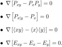
is, we must have Pxy = PxPy and hence ∇[Pxy −PxPy] = 0. Similarly, separability

re-quires we also satisfy_∇[_⟨xy_{⟩ − ⟨}x_⟩⟨y_⟩] = 0. Further, every independent space must have

conditional probabilities equal to marginal probabilities and so satisfy_∇[Px|y −Px

]

= 0. Finally, two independent variables have joint entropy equal to the sum of the individual

entropies so every independent space must satisfy _∇[Exy −Ex−Ey] = 0. These

rela-tions evaluate differently in either _Pind with isomorphism constraints or Pind′ with limit

processes. For the square die under consideration, we have probabilities and expectations of

Pxy(00)−Px(0) = ad−bc

⟨xy_{⟩ − ⟨}x_⟩⟨y_⟩ = ad₋bc

Px_|y(0|0)−Px(0) =

ad₋bc

a+c , (1.51)

and entropies of

Ex = −(a+b) log(a+b)−(1−a−b) log(1−a−b)

Ey = −(a+c) log(a+c)−(1−a−c) log(1−a−c)

Exy = −aloga−blogb−clogc−dlogd. (1.52)

The resulting gradients are

∇[Pxy(00)−Px(0)Py(0)]|ad=bc = 0 lim

∇[_⟨xy_{⟩ − ⟨}x_⟩⟨y_⟩]_|ad=bc = 0 lim

ad→bc∇[⟨xy⟩ − ⟨x⟩⟨y⟩] = adlim→bc∇(ad−bc) ̸= 0

∇[Px_|y(0|0)−Px(0)

]

|ad=bc = 0

lim ad→bc∇

[

Px|y(0|0)−Px(0)

]

= lim

ad→bc∇

[

ad₋bc a+c

]

̸

= 0

∇[Exy −Ex−Ey]|ad=bc = 0 lim

ad→bc∇[Exy −Ex−Ey] = (1.53)

lim ad→bc∇

{

alog

[ d a

a₋ad+bc d₋ad+bc ]

+blog

[ d b

b+ad₋bc d₋ad+bc ] + clog [ d c

c+ad₋bc d₋ad+bc ]

+ log

[

d₋ad+bc d

]}

̸

= 0.

1.2.4

Entropy maximization

The joint entropy Exy reflects the uncertainty between the x and y variables.

Accord-ing to probability theory, this uncertainty does not include any uncertainty about which probability space is being chosen, while conversely, according to game theory the uncer-tainty between these variables increases when it includes additional unceruncer-tainty about which probability space is being chosen.

We now present a numerical investigation of how to determine the maximum joint

entropyExy of embedded probability states featuring possibly correlated variablesx and

y as depicted in Fig. 1.3. The joint entropy is

Exy(a, b, c) =−

∑

xy

PxylogPxy. (1.54)

Using isomorphism constraints, the maximization problem is

maxExy|_ρxy=¯ρ (1.55)

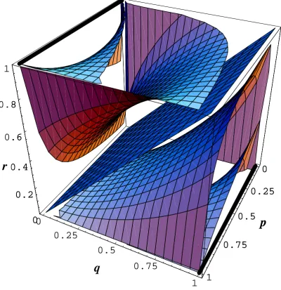
for all ¯ρ_∈[₋1,1]. Here, the correlation function betweenxandyis given by the later Eq.

2.11. This equation can be inverted to solve for the variable r as a function of p,q, and

the constant correlation ¯ρ, and the result r+(p, q,ρ¯) is given in Eq. 3.10. A numerical

optimization then generates the maximum entropy value for every correlation state ¯ρ

with the results shown in Fig. 1.4. As expected, the presence of isomorphism constraints ensures the entropy ranges from a minimum of log 2 up to a maximum of 2 log 2.

In contrast, when the joint entropy is maximized over the entire space using the tech-niques of game theory, then a single maximum outcome is achieved giving the maximum entropy in the absence of isomorphism constraints. This line is also shown in Fig. 1.4 as

1.2. OPTIMIZATION AND ISOMORPHIC PROBABILITY SPACES 19

-1 -0.5 0.5 1

Ρ

0.6 0.8 1 1.2 1.4

E

H

x, y

L

Figure 1.4: Maximizing the joint entropy of two correlated random variablesx, y _{∈ {}0,1_}.

Without isomorphism constraints, the maximum entropy is equal to 2 log 2 (dashed line). However, when subject to isomorphism constraints, the simplex will exactly reproduce the different maximum entropy states of each of its embedded probability spaces (solid line).

1.2.5

Continuous bivariate Normal spaces

The above results are general. When source probability spaces are embedded within target probability spaces, then the use of isomorphic mapping constraints will preserve all properties of the embedded spaces. Conversely, when constraints are not used then some of the properties of the embedded spaces will not be preserved in general. We illustrate this now using normally distributed continuous random variables.

Consider two normally distributed continuous independent random variables xand y

with x, y _∈(_−∞,_∞). When independent, these variables have a joint probability

distri-butionPxy which is continuous and differentiable in six variables, Pxy(x, µx, σx, y, µy, σy)

where the respective means areµx andµy and the variances areσx2 andσy2. The marginal

distributions are Px(x, µx, σx) and Py(y, µy, σy). In particular, we have

Pxy = 1 2πσxσy

e−

1 2

[₍

x−µx)2

σ2_x +

(y−µy)2

σ_y2

]

Px = 1 √

2πσx

e−

1 2

(x−µx)2

σ2_x

Py = 1 √

2πσy

e−

1 2

(y−µy)2

σ_y2

. (1.56)

The conditional distribution forx given some value of y is

Px|y = 1 √

2πσx

e−

1 2

(x−µx)2

These independent joint distributions can now be embedded into an enlarged

distri-bution representing two potentially correlated normally distributed variables x and y.

This enlarged distributionP′

xy(x, µx, σx, y, µy, σy, ρ) differs from Pxy in its dependence on

the correlation parameter ρxy =ρ with ρ∈ (−1,1). This distribution is continuous and

differentiable in seven variables. The joint distribution is

P_xy′ = 1

2πσxσy

√

1₋ρ2e

− 1 2(1−ρ2)

[₍

x−µx)2

σ2_x −

2ρ(x−µx)(y−µy)

σxσy +

(y−µy)2

σ2_y

]

. (1.58)

The marginal distributions for the correlated case are identical to those of the independent

space so P′

x =Px and Py′ =Py. The conditional distribution forx given some value of y

is

P_x′_|y = √ 1

2π(1₋ρ2_)σ

x

e−

1 2(1−ρ2)

(x−µx¯ )2

σ2_{x , (1.59)}

where the new conditioned mean is

¯

µx =µx+ρ

σx

σy

(y₋µy). (1.60)

An isomorphic embedding requires that the unit probability subset of Pxy be mapped

onto the unit probability subset of Pxy′ and this is achieved by imposing an external

constraint thatρ= 0 in the enlarged space. Hence, we expect Pxy′

_ρ

=0=Pxy. It is readily

confirmed that when the isomorphism constraint is imposed on the enlarged distribution all properties are preserved, while this is not the case in the absence of the constraint.

The gradient operator _∇is now a function of seven variables

∇ = ∂

∂xxˆ+ ∂ ∂yyˆ+

∂ ∂µx

ˆ

µx+

∂ ∂µy

ˆ

µy+

∂ ∂σx

ˆ

σx+

∂ ∂σy

ˆ

σy +

∂

∂ρρ.ˆ (1.61)

The probability distributions must satisfy a number of gradient relations, but we have:

∇[Pxy′ −Px′Py′

] _ρ

=0 = 0 lim

ρ_→0∇

[

P_xy′ ₋P_x′P_y′] = ˆρlim ρ_→0

∂ ∂ρP

′

xy ̸= 0

∇[Px′_|y −Px′

]

_ρ=0 = 0

lim ρ→0∇

[

Px′|y−Px′

]

= ˆρlim

ρ→0

∂ ∂ρP

′

x|y ̸= 0. (1.62)

Similarly, the expectations of functions of thexandyvariables must also satisfy a number

of gradient relations. As expectations integrate over the x and y variables, the gradient

operator is a function of only five variables now,

∇= ∂

∂µx ˆ

µx+

∂ ∂µy

ˆ

µy+

∂ ∂σx

ˆ

σx+

∂ ∂σy

ˆ

σy+

∂

∂ρρ.ˆ (1.63)

We have

∇[_⟨xy_⟩′_{− ⟨}x_⟩′_⟨y_⟩′]_|ρ=0 = 0 lim

ρ_→0∇[⟨xy⟩

′_{− ⟨x⟩}′_⟨y⟩′_{] = ˆρlim}

ρ_→0

∂ ∂ρ⟨xy⟩

1.2. OPTIMIZATION AND ISOMORPHIC PROBABILITY SPACES 21

1.2.6

Quantum probability spaces

As noted above, the use of isomorphic mappings to preserve the properties of probability spaces is general. As a last illustration, we show the use of isomorphic mappings when applied to quantum probability spaces.

Suppose a quantum probability space is to be embedded within another enlarged quantum probability space. (See [14] for an overview of quantum information theory

including quantum information geometry.) AnN level quantum system has von Neumann

entropy defined as

EN =−tr ˆRNlog ˆRN (1.64)

where here ˆRN is the quantum density matrix and tr indicates a trace operation applied

to a matrix. Supposing that matrix D diagonalizes the density matrix so DRˆND† is

diagonal, and that its eigenvalues are λi for 1≤i≤N, we have

EN =− N

∑

i=1

λilogλi. (1.65)

The eigenvalueλi specifies the occupancy probability of theith level. Hence, maximizing

the N-level system entropy requires that λi = 1/N for all i. Consequently, a two level

quantum system maximizes its entropy E2 when the density matrix is an equiprobable

mixture equal to half of the two level identity matrix, ˆR2 = 1/2I2, while a three level

quantum system maximizes its entropy E3 when the density matrix is an equiprobable

mixture of ˆR3 = 1/3I3.

Now, if the two level system were isomorphically embedded within a three level system,

then the two level system entropy E2 is properly maximized only when isomorphism

constraints are used to decouple the third level so that it plays no part in the optimization.

This is achieved by using an isomorphism constraint λ3 = 0 to decouple and remove the

third level from the system. That is, the optimization taking account of an isomorphism

constraint _∇3E3|λ3=0 = 0 will determine the correct maximum value for E2. However,

a failure to use an isomorphism constraint will locate an incorrect maximum point via

limλ3→0∇3E3. We have

∇2E2 =∇3E3|λ3=0 ̸= lim

λ3→0∇3

E3. (1.66)

Isomorphism constraints must be used to properly embed one quantum probability space within another.

1.2.7

Perfect correlation reduces dimensionality

Standard probability theory holds that when two variables x and y are known to be

perfectly correlated, thenP(x, y) =P(x)P(y_|x) = P(x). That is, any optimization which

involves the joint distribution P(x, y) does not involve two dimensions but only one as

x = y. Perfect correlation reduces dimensionality which alters the gradient operators

HbL XPX_@PX_HxL,PY_HyLD\

X_PY_@PX_HxL,PY_HyLD\

PX_HxL

PYHyL

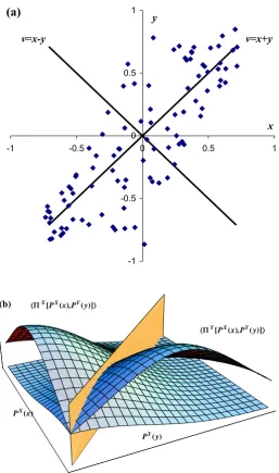
Figure 1.5: (a) An affine transformation of correlated variables x and y generates new

orthogonal variables u = x+y and v = x₋y which are uncorrelated. (b) When x and

y are perfectly correlated, v = 0 and u is the only free variable and dimensionality is

reduced. Optimization solutions must lie on the u-axis satisfying the constraint x=y.

Probability theory takes account of this dimensionality reduction when using Affine variable transforms. Typical presentations of probability theory hold that “any two

real-valued random variables x and y whose mean values and variances exist may be

represented as an Affine transformation of a pair of uncorrelated random variables” [15]. Such statements, carelessly interpreted, would indeed suggest that perfect correlations involve no reduction in the number of variables. Writing the respective mean values as

⟨x_⟩ and _⟨y_⟩, and defining the translated variables

x∗ = x_{− ⟨}x_⟩

1.2. OPTIMIZATION AND ISOMORPHIC PROBABILITY SPACES 23

then an affine transformation can always be used to define two new variables

u = x∗+y∗

v = x∗₋y∗. (1.68)

These variables each have mean zero, _⟨u_⟩=_⟨v_⟩= 0, and are uncorrelated as

cov(u, v) = _⟨uv_⟩= 0. (1.69)

The zero covariance results from the orthogonality of the random variables u and v in

a suitable L2 _{vector space, while the possibly correlated original variables are generated}

from the inverse affine transformation

x = σxx∗+⟨x⟩ =

σx

2 (u+v) +⟨x⟩

y = σyy∗+⟨y⟩ =

σy

2 (u−v) +⟨y⟩, (1.70)

where here, σz is the standard deviation of variablez ∈ {x, y}.

If the xandy variables are perfectly correlated, thenv is identically zero and uis the

only surviving variable. Perfect correlations reduce the dimensionality of the optimization space and probability theory preserves the dimensionality of perfectly correlated variables when using Affine transforms. (See Fig. 1.5.)

A similar preservation of dimensionality occurs in the Hotelling transform, a discrete version of the Karhunen-Lo`eve transform [16]. This transform can also be used to map

the probability space of two uncorrelated centered variables (u, v) into the probability

space of two correlated centered variables (x, y). If the state of correlation betweenxand

y is ρ, then the Hotelling transform is implemented via



 x y



=





1 0

ρ √1₋ρ2



 

 u v



. (1.71)

Then, whenever thexandyvariables are not perfectly correlated both the (u, v) and (x, y)

probability spaces are two dimensional. However, when ρ= 1 and x and y are perfectly

correlated, then the mapping matrix becomes singular and non-invertible ensuring that

x = y = u so that the x and y probability space is one dimensional even while the u

andv probability space is two dimensional. Probability theory again acts to preserve the

dimensionality of the joint probability space of perfectly correlated variables.

1.2.8

Example isomorphic functions

There are different ways to embed a smaller source function within an enlarged target function which can preserve different amounts of the structure of the source function within the target function. Consider for example, mapping a 1-dimensional function

One way to implement this assignment is to use limit processes constraining most of the

neighbourhood of g(x, y) in the vicinity of the line y=x to satisfy

lim

y_→xg(x, y) =f(x). (1.72)

Another way to do this is to ignore the values of g(x, y) away from the line y = x and

simply use externally imposed constraints forcing the assignment on the line via

g(x, y)_|y=x =f(x). (1.73)

This approach does not care about valuesg(x, y) whenx_̸=y. The question then is, under

what circumstances can limy_→xg(x, y) or g(x, y)|y=x be used to examine the properties

of f(x).

Hereinafter, for concreteness we will consider the simplified example functionsf(x) =

x2 _{and g(x, y) = xy. Each of the implementations, lim}

y_→xg(x, y) or g(x, y)|y=x, have different domains (dom) in each space, and hence different integration volume elements (dv)

f(x) limy→xg(x, y) g(x, y)|y=x

dom _{ℜ ℜ × ℜ ℜ}

dv dx dx dy dx.

(1.74)

The different dimensionalities of the domains impacts on any attempt to change

vari-ables within each space. The rank of the change of variable transforms (A) and the

dimensionality of the Jacobian matrices (J) in each space are

f(x) limy→xg(x, y) g(x, y)|y=x

rank(A) 1 2 1

dim(J) 1 2 1.

(1.75)

These differences impact on the evaluation of other properties such as gradients, which should evaluate as

∇f(x) = 2xxˆ (1.76)

where a hatted variable denotes a unit vector in the indicated direction. In contrast, the gradient evaluated using a limit assignment gives

∇g(x, x) = lim

y_→x∇g(x, y) = x(ˆx+ ˆy), (1.77)

which does not satisfy the required relation. Conversely, the use of an externally imposed constraint ensures

∇g(x, y)_|y=x =∇g(x, x) = 2xxˆ (1.78)

as required.

In summary, the definitions

f(x) =g(x, y)_|y=x = lim

1.2. OPTIMIZATION AND ISOMORPHIC PROBABILITY SPACES 25

do not generally carry over to the gradient relations, as

∇f(x) =_∇g(x, y)_|y=x ̸= lim

y→x∇g(x, y), (1.80)

This results as the limit process f(x) = limy_→xg(x, y) treats the x and y variables as

being independent and simply evaluates desired quantities at points (x, y) lying on the

line y = x. In contrast, the constraint f(x) = g(x, y)_|y=x enforces a functional relation

between the x and y variables which preserves all the structures of f(x) within g(x, x).

It is well understood that any functional relation between the variables of a function will impact on the properties of that function. Such functional relations must be preserved whenever that function is mapped into a different space. The need to take account of such functional relations is a standard part of routine optimization techniques such as differentiation via any of the chain rule, Lagrangian multipliers, or directed vector gradients.

A number of standard techniques exist for evaluating the gradient f′_{(x) using the}

constrained function g(x, y)_|y=x. For instance, the chain rule can be applied to the

functions g(x, y) andy(x) = x giving

f′(x) = ∂g

∂x + ∂g ∂y

dy dx

= 2xx.ˆ (1.81)

Another common alternative is by using Lagrange multipliers in which f′_{(x) = L}′_(x)

with

L(x, y, λ) =xy₋λ(y₋x) (1.82)

and

∂L

∂x = (y+λ)ˆx ∂L

∂y = (x−λ)ˆy ∂L

∂λ = (x−y)ˆλ. (1.83)

Equating the last two lines to zero gives the required constraints y = x and λ = x

ensuring f′_{(x) = L}′_{(x). A final way to perform this constrained optimization is to use}

directed vector gradients where

f′(x) = lim

y→x∇g(x, y).v.

√

2 (1.84)

withv = (ˆx+ ˆy)/√2. Here,v is normalized and the extra factor of√2 properly calculates

changes in the x direction. This gives the magnitude of the gradient as f′_{(x) = 2x as}

required.

There are two ways to embed the function f(x) within the surfaceg(x, y) using either