Two stage weighted least squares estimator of the conditional mean of observation driven time series models

Munich Personal RePEc Archive

Two-stage weighted least squares

estimator of the conditional mean of

observation-driven time series models

Aknouche, Abdelhakim and Francq, Christian

USTHB and Qassim University, University of Lille and CREST

1 December 2019

Online at

https://mpra.ub.uni-muenchen.de/97382/

Two-stage weighted least squares estimator of the

conditional mean of observation-driven time series

models

Abdelhakim Aknouche

and Christian Francq

Abstract

General parametric forms are assumed for the conditional meanλt(θ0) and variance

υt(ξ0) of a time series. These conditional moments can for instance be derived from

count time series, Autoregressive Conditional Duration (ACD) or Generalized

Autore-gressive Score (GAS) models. In this paper, our aim is to estimate the conditional

mean parameter θ0, trying to be as agnostic as possible about the conditional

distri-bution of the observations. Quasi-Maximum Likelihood Estimators (QMLEs) based

on the linear exponential family fulfill this goal, but they may be inefficient and have

complicated asymptotic distributions whenθ0 contains zero coefficients. We thus study

alternative weighted least square estimators (WLSEs), which enjoy the same

consis-tency property as the QMLEs when the conditional distribution is misspecified, but

have simpler asymptotic distributions when components ofθ0 are null and gain in

effi-ciency whenυt is well specified. We compare the asymptotic properties of the QMLEs

and WLSEs, and determine a data driven strategy for finding an asymptotically

opti-mal WLSE. Simulation experiments and illustrations on realized volatility forecasting

are presented.

∗_{University of Science and Technology Houari Boumediene, and Qassim University.} †_{Corresponding author, CREST and University of Lille, e-mail: [email protected].}

Keywords: Autoregressive Conditional Duration model; Exponential, Poisson, Negative

Binomial QMLE; INteger-valued AR; INteger-valued GARCH; Weighted LSE.

JEL Classification: C13, C32, C53, C58.

1

Estimating the conditional mean

Consider a real-valued stochastic process {Xt, t∈Z_{}. Let Ft be the sigma-field generated}

by_{Xu, u_≤t_}. Assume a parametric form for the conditional mean :

E(Xt| Ft−1) =λ(Xt−1, Xt−2, ...;θ0) =λt(θ0) =λt, t∈Z. (1.1)

Important classes of count time series models, in particular the Poisson INteger GARCH

(INGARCH), the Negative Binomial INGARCH and the INteger AR (INAR), that will be

considered in Section 3 below, have a conditional mean of the form (1.1). The most frequent,

and maybe most natural, specification forλt is the INGARCH(p, q)-type equation

λt =ω0+

q

X

i=1

α0iXt−i+ p

X

j=1

β0jλt−j. (1.2)

For the INAR models, the conditional mean has also the parametric form (1.2), with p= 0.

In (1.2) the unknown parameter is θ0 = (ω0, α01, . . . , β0p). For modeling positive time series,

such as durations or volumes, Engle and Russell (1998) proposed the ACD model of the form

Xt=λtzt, (1.3)

where (λt) satisfies (1.2) and (zt) is an iid sequence of positive variables of mean 1, for

instance of exponential distribution of rate parameter 1. Standard ARMA models are also

of the form Xt =λt+ǫt with (ǫt) an iid noise and λt satisfying (1.2).

Time series models with linear conditional mean (1.2) are thus very frequent. A drawback

of this linear specification is that it is very sensitive to large ”outliers” in Xt−i. Following

Creal, Koopman and Lucas (2011, 2013), Harvey (2013) and Blasques, Koopman, Lucas

(2015), Generalized Autoregressive Score (GAS) alternative updating equations can be

of degree of freedom ν0 > 2, standardized in such a way that Ezt2 = 1, the GAS approach

developed in Harvey and Chakravarty (2008) leads to the Beta-t-ACD model1 _{in which}

λt=ω0+β0λt−1+α0

ν0+ 1

ν0−2 + Xt_λt−1

−1

Xt−1. (1.4)

When ν0 is large, this equation is close to an INGARCH(1,1), but when ν0 is small or

moderate,λtis less sensitive to an extreme value ofXt−1 in Model (1.4) than in Model (1.2),

which can be a highly desirable robustness property. As far as possible, we thus prefer to

consider the general model (1.1) than the linear specification (1.2).

Estimating θ0 is obviously of primary importance, in particular for predictingXt+h given

Ftforh≥1. The maximum-likelihood estimator (MLE) is often readily computable – except

for parameter-driven models like the INAR model (see Cox, 1981) – but it requires to specify

a conditional distribution. Each parametric specification of the conditional distribution

function (cdf) leads to a parameterization of the conditional variance (when existing)

Var (Xt_{| F}t−1) =υ(Xt−1, Xt−2, ...;ξ0) =υt(ξ0) = υt. (1.5)

In practice, the choice of the cdf is an issue. There exists actually no natural choice for

the cdf, or even for the conditional variance (1.5). For example, for count time series, the

choice of the Poisson distribution with intensity λt entails υt =λt, and is thus questionable

since it has been empirically observed that numerous count time series exhibit conditional

overdispersion (see e.g Christou and Fokianos, 2014). For positive observations, the ACD

model (1.3) entails a conditional variance proportional to the square of the conditional mean,

υt =λ2

t(Ezt2−1). An additive ARMA-type model of the formXt=λt+ǫt entails a constant

conditional variance υt = Eǫ2

t. In practice, one can easily conceive that the conditional

variance may have other forms. Obviously, the choice of a wrong cdf may affect the efficiency,

or even the consistency, of the misspecified MLE.

In the present work, we focus on the estimation of the parameter θ0 of the conditional

mean (1.1), without assuming a specific form for the cdfFθof the observations. In particular,

1_{The original version of this model was proposed for GARCH, but the ACD version is direct because an}

we are interested in estimators that could be consistent even if the conditional variance (1.5)

is misspecified. Since the works of Wedderburn (1974) and Gouri´eroux, Monfort and Trognon

(1984), it is known that, under general regularity conditions, a MLE is a QMLE – that is a

MLE based on a cdf Fθ which remains consistent when the true cdf is not Fθ – if and only

if Fθ is a particular member of the linear exponential family (defined by (2.19) below). For

positive observations X1, . . . , Xn, an example of such misspecification-consistent estimator

is the Exponential QMLE (EQMLE), defined by

b

θE = arg min

θ∈Θ

n

X

t=1

n

Xt/eλt(θ) + logeλt(θ)o, (1.6)

where Θ denotes the parameter space and λte(θ) =λ(Xt−1, . . . , X1,Xe0,Xe−1, . . .;θ) for given

initial valuesXe0,Xe−1, . . . This estimator coincides with the MLE when the cdf of the

obser-vations is the exponential distribution of parameter rate 1, but the EQMLE is consistent and

asymptotically normal (CAN) for a much broader class of cdf’s (see Aknouche and Francq,

2019). Another example of QMLE is the Poisson Quasi-MLE (PQMLE), defined by

b

θP = arg max

θ∈Θ

n

X

t=1

n

Xtlogeλt(θ)−eλt(θ)o. (1.7)

This estimator, which coincides with the MLE when the cdf of the observations is Poisson

Pλt, is CAN for the mean parameter of count time series (see Ahmad and Francq, 2016)

or duration-type (see Aknouche and Francq, 2019) models. However, this estimator is in

general inefficient whenυt6=λt. Motivated by the existence of overdispersed series for which

υt > λt, Aknouche, Bendjeddou and Touche (2018) studied the profile Negative Binomial

QMLE (NBQMLE), defined by

b

θN B = arg max

θ∈Θ

n

X

t=1

Xtlog eλt(θ)

r+eλt(θ)

!

−rlognr+eλt(θ)o, (1.8)

where the parameter r is fixed. An intuition for the CAN of the QMLEs is obtained by

looking at the first order conditions. Any QMLE θbsatisfies

sn(θb) = 0, sn(θ) =

n

X

t=1

Xt₋eλt(θ)

e

υt(θ)

∂eλt(θ)

where _eυt(θ) is an approximation of the conditional variance υt of a given member of the

exponential family. For the Exponential, Poisson and Negative Binomial QMLE, we have

respectively _eυt(θ) = eλ2t(θ), eυt(θ) = λet(θ) and υet(θ) = eλt(θ)(1 + eλt(θ)/r). Each of these

estimators is optimal within the class of the QMLEs when the conditional varianceυtis well

specified. The possible value of υt is however restricted by the fact that it must match the

conditional variance of an exponential family distribution. For example, it is not possible to

have υt = λt or υt =λ2t when the support of the observations is R (see Table 1 in Morris,

1982).

The aim of this paper is to propose and study alternative estimators which enjoy the

same consistency property as the QMLEs when the cdf is misspecified, but gain in efficiency

when υt is well specified.

Given a theoretical weight function wt = w(Xt−1, Xt−2, . . .), where w is a measurable

function from R∞ _{to (0,∞), and its observation-proxy}

e

wt=w(Xt−1, . . . , X1,Xe0,Xe−1, . . .)≥w >0, (1.10)

a first weighted least square estimator (WLSE) is defined by

b

θ1W LS = arg min

θ∈ΘLne (θ,we), (1.11)

where

e

Ln(θ,w_e) = 1

n n

X

t=1

elt(θ,wt_e) with elt(θ, wt) = (Xt−eλt(θ))

2

wt . (1.12)

The role of the weighting sequence w_e = (wt_e)_t≥1 is twofold: it allows the WLSE to be CAN

without too strong moment conditions, and it may reduce the asymptotic variance of the

estimator.

As will be seen in Section 2, the optimal choice of w_e is (proportional to) υ = (υt)_t≥1. In

practice, the actual value of υt is generally unknown. Assuming for the conditional variance

a parametric specification of the form

υ∗

(Xt−1, Xt−2, ...;ξ0∗) =υ

∗

t(ξ

∗

the optimal sequence of weights may be estimated by

{wt,nb }t, wt,nb =υ

∗

Xt−1, Xt−2, ..., X1,Xe0,Xe−1, . . .;ξnb

, (1.14)

where ξnb is a first-step estimator of ξ∗

0 (which is often function of the estimator bθ1W LS of

θ0, and possibly of estimates of some extra parameter ς0). This leads to a two-stage WLSE,

defined by

b

θ2W LS = arg min

θ∈ΘLne θ,{wt,nb }t

. (1.15)

We will see that, even when the conditional variance is misspecified (i.e. υ∗

t(ξ

∗

0) 6= υt), the

two-stage estimator θb2W LS is a consistent estimator of θ0 under mild regularity conditions.

For an informal comparison with the QMLEs, note that the first order conditions entail

sn(θb2W LS) = 0, sn(θ) = n

X

t=1

Xt−eλt(θ)

b

υt

∂eλt(θ)

∂θ , (1.16)

whereυt_b =wt,n_b is a first-step estimator of υt. The main difference with (1.9) is that there is

particular constraint on the conditional variance. We will see that this can lead to efficiency

gains of the WLSE compared to QMLEs.

The rest of the paper is organized as follow. Section 2 provides general regularity

con-ditions for CAN of the WLS estimators and compares these estimators with the MLE and

QMLEs. In Section 3, more explicit CAN conditions are given for particular time series

mod-els. Section 4 proposes a method to select one estimator within a set of possible WLSEs.

Monte Carlo experiments and illustrations on real data sets are presented in Section 5. Proofs

are collected in Section 6.

2

Asymptotic behavior of the WLS estimators

Using a WLSE of the form (1.11), we assume that λ : R∞

×Θ _→ (_−∞,_∞) is a known

measurable function satisfying (1.1), with θ0 an unknown parameter belonging to some

compact parameter space Θ_⊂Rm_{. The WLSEs are semi-parametric estimators in the sense}

2.1

CAN of the estimators

The CAN of the WLSE can be shown under the following assumptions.

A1 There exists a strictly stationary and ergodic process_{Xt, t_∈N_{} satisfying (1.1).}

A2 Lettingat = supθ∈Θ

eλt(θ)−λt(θ), a.s. limt→∞{sup_θ∈Θ|λt(θ)|+|Xt|+ 1}at= 0.

A3 λt(θ) =λt(θ0) a.s. if and only if θ=θ0.

A4 Almost surely, as t→ ∞

|wt−wte|

1 +X_t2+ sup

θ∈Θ

λ2_t(θ)

→0.

A5 Eυ1

w1

<∞with υt= Var (Xt | Ft−1).

A6 The matricesI(θ0, w) = E

υt w2

t

∂λt(θ0)∂λt(θ0)

∂θ∂θ′

andJ(θ0, w) = E

1

wt

∂λt(θ0)∂λt(θ0)

∂θ∂θ′

exist

and J(θ0, w) is invertible.

A7 Almost surely, the function λt(_·) admits continuous second-order derivatives in a

neighbourhood V (θ0) of θ0, and we have Ew−t1 sup

θ∈V(θ0)

{Xt−λt(θ)}2 <∞,

Ew−1

t sup θ∈V(θ0)

∂2_λt(θ)

∂θ∂θ′ 2

<_∞ and Ew−1

t sup θ∈V(θ0)

∂λt(θ)

∂θ

∂λt(θ)

∂θ′

<∞. (2.1)

A8 Lettingbt= supθ∈Θ

∂eλt(θ)/∂θ−∂λt(θ)/∂θ

, the sequences

bt

|Xt_|+ sup

θ∈Θ|

λt(θ)_|

, atsup

θ∈Θ

∂λt_∂θ(θ)

, |wt−wte|sup_θ∈Θ ∂λt_∂θ(θ)

|Xt_|+ sup

θ∈Θ|

λt(θ)_|

are a.s. of orderO(t−κ_{) for some κ >1/2.}

A9 The true parameter θ0 belongs to the interior

◦

Θ of Θ.

Assumptions A1–A3 are used by Ahmad and Francq (2016) for showing the consistency of

the PQMLE in the case of count time series. AssumptionsA2andA4are used to show that

the initial values Xe0,Xe−1, . . . are asymptotically unimportant. The choice of the weight

function wt is guided by A5. If υt is assumed to be (bounded by) a linear function of

|Xt−1|, . . . ,|Xt−r|, then A5 is automatically satisfied if, for instance, wt = 1 +Pr_i=1|Xt−i|.

If wt is chosen to be constant then the moment condition EX2

t < ∞ is required. These

assumptions will be made more explicit in specific examples discussed in Section 3 below.

Remark 2.1 (The WLS estimators avoid boundary problems) Consider the case of

positive observations (for instance (Xt) represents a time series of counts or volumes). For

the estimators in (1.6)–(1.8) be well defined, it is necessary to be able to computelogλet(θ)

for all θ _∈Θ. For this reason, the condition

λ: [0,_∞)∞

×Θ_→[λ,_∞) for some λ >0 (2.2)

is imposed for these QMLEs. In the INGARCH case (1.2), the latter condition is satisfied

by imposing ω _≥ λ, αi ≥ 0 and βj ≥ 0. Indeed, if for instance α < 0 is allowed, then

λt(θ) := ω+αXt−1+βλt−1(θ) can take negative values with non zero probability, and the

QMLEs may fail. When one or several coefficients in (1.2) are equal to zero, θ0 thus lies at

the boundary of Θ, and A9 is not satisfied. In this situation, appearing in particular when

testing the significance of the INGARCH coefficients, Ahmad and Francq (2016) showed that

the PQMLE has a non Gaussian asymptotic distribution, which entails serious practical

difficulties. For the WSLE, it is possible to have eλt(θ) <0 for some values of θ—although

we must have λt(θ0) ≥ 0 for positive observations—and thus A9 may hold even if θ0 has

zero components (see Section 3.1).

Theorem 2.1 Under the assumptions A1-A5, and (1.10)

b

θ1W LS →θ0 a.s. as n→ ∞. (2.3)

If in addition A6-A9 hold, as n _{→ ∞}

√

nθb1W LS −θ0

_d

→ N(0,Σ) Σ = Σ (θ0, w) =J−1(θ0, w)I(θ0, w)J−1(θ0, w). (2.4)

Note that the consistency of the two-stage WLSE cannot be directly deduced from that

of the one-step WLSE because, contrary to wt, wt,n_b is not _Ft-measurable. Let υe∗t(ξ) =

υ∗

Xt−1, Xt−2, ..., X1,Xe0,Xe−1, . . .;ξ

, so thatwt,n_b =υ_e∗

t(ξnb), and letwt =υ∗t(ξ0∗). From now

on, K denotes a generic positive constant, or a positive random variable_F0-measurable, and

ρ a generic constant belonging to [0,1). For consistency of the two-stage WLSE, we replace

A4∗ _{There exists σ > 0 such that, almost surely, w}

t > σ and wbt,n > σ for n large

enough. Assume ξnb is a strongly consistent estimator of ξ∗

0, the function υt∗(·) is almost

surely continuously differentiable,

sup

ξ∈V(ξ∗

0)

|υe∗

t(ξ)−υ

∗

t(ξ)| ≤Kρt and E

1

wtξ∈supV(ξ∗

0)

∂υ

∗

t(ξ) ∂ξ

sup_θ∈Θ{Xt−λt(θ)}2 <∞, (2.5)

where V(ξ∗

0) is a neighborhood of ξ

∗

0. Moreover, assume

Esup

θ∈Θ|

Xt₋λt(θ)_|s <_∞ for some s >0. (2.6)

To show the asymptotic normality, we need to slightly modify other assumptions. First

of all, when υt is well specified, A6 simplifies as follows.

A6∗ _{The matrix I =E}1

υt

∂λt(θ0)∂λt(θ0)

∂θ∂θ′

exists and is invertible.

LetA7∗

be obtained by adding inA7 the assumption that √nξnb −ξ∗

0

=OP(1) and

E 1 wt

sup

ξ∈V(ξ∗

0)

∂υ∗

t(ξ) ∂ξ

2"

1 + sup

θ∈V(θ0)

{Xt₋λt(θ)_}2

#

<_∞. (2.7)

Let A8∗ _{be the assumption obtained by replacing}

|wet−wt| by supξ∈V(ξ∗

0)|eυt(ξ)−υt(ξ)| in

A8, for some neighborhood V(ξ∗

0) ofξ

∗

0.

The following theorem establishes the asymptotic distribution of the two-stage WLSE

when the conditional variance is well specified (i.e. υ∗

t(ξ

∗

0) = υt) or when it is misspecified,

and shows its relative efficiency with respect to the one-step WLSE under correct specification

of υt.

Theorem 2.2 Under A1-A3, (1.10), A4∗ _{and A5 (which is satisfied when υ}

t is well

spec-ified)

b

θ2W LS →θ0 a.s. as n→ ∞. (2.8)

Under the previous assumptions and A6, A7∗

, A8∗

and A9, as n → ∞,

√

nθb2W LS −θ0

_d

If in addition the conditional variance is well specified up to a positive constant, that is (1.5)

and (1.13) hold with ξ∗

0 =ξ0 and υ∗(·) =kυ(·) for some k >0, then A6 can be replaced by

A6∗ _and

√

nθb2W LS −θ0

_d

→ N 0, I−1 _{as n}

→ ∞. (2.10)

Moreover the matrix Σ₋I−1 _{is positive semi-definite.}

2.2

The linear conditional mean case

Assume that Xt ≥ 0 almost surely and that the conditional distribution of Xt given Ft−1,

denoted byFλt, depends on its conditional meanλt (and maybe of other fixed parameters).

Consider the case where λt follows the linear model (1.2). We assume that the stochastic

order of the cdf increases with its mean. More precisely, let Fλ be a family of cumulative

distribution functions indexed by the mean λ = R ydFλ(y) ∈ [0,∞). Assume that, within

this family, the stochastic order is equal to the mean order, i.e.

λ≤λ∗ ⇒ Fλ(x)≥Fλ∗(x), ∀x∈R. (2.11)

Aknouche and Francq (2019) showed that ifP(Xt≤x| Ft−1) = Fλt(x) andλtsatisfies (1.2),

then A1 holds true when _{Fλ, λ_∈(0,_∞)_} satisfies (2.11) and

q

X

i=1

α0i+ p

X

j=1

β0j <1. (2.12)

Moreover, the solution is such thatEXt<_∞. By Remark 2.1 in Ahmad and Francq (2016),

Assumption A2 is satisfied when

p

X

j=1

βj <1 for all θ _∈Θ. (2.13)

In the latter reference, it is also shown that A3 is satisfied if q >0 and

Aθ0(z) :=

q

X

i=1

α0izi and Bθ0(z) := 1−

p

X

i=1

β0izi have no common root,

Now suppose that the weighting sequence w_e is defined by

e

wt=c+aXt−1+bwte−1

with c >0, a >0 andb ∈(0,1). We thus have wt =P∞_i=0bi_(c+aXt

−i−1) and

wt−wte =bt−1(w1−we1) = bt−1

∞

X

i=0

biaX−i−Xe−i

with, for instance, Xet = 0 for t ≤ 0, and thus we1 = c. By the Borel-Cantelli lemma, it is

then easy to show that A4 holds true. It is also clear that A4 holds true for many other

forms of the weighting sequence w_e. Assumptions such as A5, as well as the choice of the

weighting sequence for the two-stage estimator, depend on the particular form ofFλ and are

thus discussed in Section 3 below.

Let us discuss the other assumptions in the case p = q = 1, the results extending to

general orders p and q with the same arguments but heavier notations. We have

λt(θ)−eλt(θ) =βnλt−1(θ)−eλt−1(θ)

o

=βt−1

∞

X

i=0

βiαX−i−Xe−i

and

∂λt(θ)

∂θ =

    

1

Xt−1

λt−1(θ)

    +β

∂λt−1(θ)

∂θ .

This entails that

at≤Kρt, bt≤Ktρt, sup θ∈Θ|

λt(θ)| ≤K

∞

X

i=0

ρi_{{1 +|X} t−i|}

and

sup

θ∈Θ

∂λt(θ) ∂θ

+ sup_θ∈Θ

∂2_λ

t(θ) ∂θ∂θ′

≤K

∞

X

i=0

ρi

1 +|Xt−i|+ sup θ∈Θ|

λt−i(θ)|

. (2.15)

It follows that, for all weighting sequence satisfying (1.10) and A4, Assumptions A7 is

satisfied whenever EX2

t <∞. By the Borel-Cantelli lemma and Markov inequality, we also

deduce that, for weighting sequences satisfying

A8is satisfied under the same moment condition. The existence ofI(θ0, w) for any sequence

wt _≥ w > 0 is ensured by the moment condition EX4

t < ∞. By the arguments given

in Remark 2.3 of Ahmad and Francq (2016), J(θ0, w) is invertible under the identifiability

condition (2.14). Assumptions A6 is thus satisfied when EX4

t < ∞. When the weighting

sequence is optimally chosen, the moment conditions are weaker. In particular Assumptions

A6∗ _{is satisfied when EX}2

t <∞. Now let us further discuss Assumption A9, for simplicity

in the case p=q = 1. For the reasons given in Remark 2.1, for computing the PQMLE the

components of θ must be positively constrained, so that (2.2) holds true. The parameter

space of the PQMLE is thus typically chosen of the form

Θ = [ω, ω]×[0, α]×[0, β], (2.17)

with 0< ω < ω, 0< α and 0 < β <1 (the last inequality ensuring (2.13)). The WLS

esti-mators can be computed without imposing any positivity constraints, so that the parameter

space can be chosen, for instance, of the form

Θ = [₋ω, ω]_×[₋α, α]_×[₋β, β]. (2.18)

When Θ is like (2.17), AssumptionA9 is quite restrictive because it precludes, in particular,

a parameter of the form θ0 = (ω0, α0,0), i.e. the interesting situation where the DGP is an

Integer ARCH (see Section 3.4 below). On the contrary, for Θ of the form (2.18), Assumption

A9 is always satisfied, provided ω, α and β are chosen large enough.

2.3

Optimality of the 2WLSE

UnderA1-A3, assumptions similar toA6-A8, and A9with (2.2) (see Remark 2.1), Ahmad

and Francq (2016) established CAN of the PQMLE in the case of integer-valued observations.

They showed that

√

nbθP ₋θ0

_L

→

n→∞N (0,ΣP), ΣP =J −1

P IPJ

−1

P

with

IP =Eυt(θ0)

λ2

t(θ0)

∂λt(θ0)∂λt(θ0)

∂θ∂θ′

and JP =E_λt(1_θ0)∂λt(θ0)∂λt(θ0)

∂θ∂θ′

Note thatIP =I(θ0, ω) andJP =J(θ0, ω) withω ={λt}. In the same framework, Aknouche

et al. (2018) showed that under certain regularity conditions we have

√

nbθN B−θ0

_L

→

n→∞N(0,ΣN B), ΣN B = Σ(θ0, ω), ω ={λt(1 +λt/r)}.

For positive observations Aknouche and Francq (2019) gave conditions for

√

nθEb ₋θ0

_L

→

n→∞ N(0,ΣE), ΣE = Σ(θ0, ω), ω=

λ2_t .

Note that, as for the last one, the CAN of the first 2 QMLEs is valid not only for count

series but also for positive data in general (see Remark 4.1 in Aknouche and Francq, 2019).

The optimal WLSE is never asymptotically less efficient than a QMLE.

Corollary 2.1 Assume Xt _≥0 almost surely and the CAN of the WLSEs and QMLEs. If

the conditional variance is well specified, the two-stage WLSE is asymptotically more efficient

than the QMLEs, in the sense that the matrices ΣP −I−1, ΣN B−I−1 andΣE −I−1 are all

positive semi-definite.

We now show that θb2W LS is asymptotically efficient when the true cdf of Xt belongs to the

versatile class of the linear exponential distributions. With respect to some σ-finite measure

µ(in general the Lebesgue measure or the counting measure), let fλ be the density of a real

random variable of meanλ =R fλ(x)dµ(x). Let Λ be a nonempty open subspace of R_{. It is}

said that the set_{fλ, λ_∈Λ_} constitutes a one-parameter linear exponential family if for all

λ∈Λ

fλ(x) = h(x)eη(λ)x−a(λ)_{, (2.19)}

for some two times differentiable functionsη(_·) anda(_·). For examplefλ can be the

Exponen-tial density of rate parameter 1/λ=−η, or the Poisson distribution with intensity parameter

λ=eη_{, or the negative binomial distribution with parametersr andp=r/(λ+r), assuming}

that r is fixed.

Corollary 2.2 AssumeA1whereλt(·)admits continuous second-order derivatives. Suppose

given λt =λ has the linear exponential form (2.19), and that λt(θ0) belongs almost surely

to the interior of Λ. The optimal two-stage WLSE is then asymptotically as efficient as the

MLE of θ0.

To apply Theorem 2.2, it is necessary to estimate the matrix Σ involved in (2.9). This

can be done by using the empirical estimator Σ =b Jb−1_IbJb−1_{, where}

b

J = 1

n n

X

t=1 1

b

wt,n

∂eλt(θb2W LS) ∂θ

∂eλt(θb2W LS)

∂θ′ , (2.20)

b

I = 1

n n

X

t=1

n

Xt₋eλt(θb2W LS)

o2

b

w2

t,n

∂eλt(θb2W LS) ∂θ

∂eλt(θb2W LS)

∂θ′ . (2.21)

To estimate the matrix Σ involved in (2.4), it suffices to replace w_bt,n and θe2W LS bywt and

e

θ1W LS in the previous matrices.

3

Application to particular models

We now give primitive conditions ensuring CAN of the WLS estimators for some specific

count time series models, an ACD model and a GAS model. We compare the relative

asymptotic efficiency of the WLSE with respect to the MLE and QMLEs.

3.1

The Poisson INGARCH model

A leading example of count time series satisfying (1.1) is the Poisson Integer GARCH model

proposed by Heinen (2003), in which the distribution of Xt conditional on Ft−1 is Poisson

P(λt) with intensity parameter λt=λt(θ0) of the form (1.2), whereω0 >0, α0i ≥0,β0j ≥0.

Ferland etal (2006) showed that under the condition (2.12) there exists a strictly stationarity

solution to the Poisson INGARCH model. The ergodicity of the solution has been shown by

Davis and Liu (2016). As discussed in Section 2.2, the result is not only true for the Poisson

cdf, but for any class of conditional distributions satisfying (2.11). Note also that under the

condition (2.12) we have EXr

Eυt = Eλt < ∞ under (2.12), A5 is satisfied for any sequence of weight wt > 0. Using

Section 2.2 and Theorem 2.1, we thus have the following result.

Corollary 3.1 Assume that Xt _{| F}t−1 ∼ P(λt) where λt =λt(θ0) follows (1.2) with (2.12)

and (2.14). Assume θ0 ∈Θ with (2.13). For any sequence of weights (wt) satisfying (1.10)

and (2.16), the WLSE is strongly consistent in the sense (2.3). When θ0 ∈

◦

Θ the estimator

is asymptotically normal, in the sense (2.4).

For the two-stage estimator, let us take the weighting sequencewt,n_b =eλtθb1W LS

(which

satisfies (1.10) and (2.16)). We then set bθ2W LS =θb2(PW LS) where

b

θ(₂P_{W LS}) = arg min

θ∈Θ

n

X

t=1

Xt−eλt(θ)2

b

wt,n , wbt,n=eλt

b

θ1W LS

. (3.1)

Using Section 2.2 and Theorem 2.2, it is easy to verify that we have the following result.

Corollary 3.2 Under the assumptions of Corollary 3.1, and if Θis chosen sufficiently large

so that θ0 ∈

◦

Θ, the 2-stage WLSE θb₂(P_{W LS}) is CAN with asymptotic variance

Σ =E 1

λt(θ0)

∂λt(θ0)∂λt(θ0)

∂θ∂θ′

−1

.

Note that, in accordance with Corollary 2.2,θb(₂P_{W LS}) has the same asymptotic distribution as

the (PQ)MLE under A9. When one or several coefficientsα0i or β0j are equal to zero, the

CAN of the 2WLSE may still hold (if Θ is chosen large enough), whereas the asymptotic

distribution of the (PQ)MLE is more complicated (see the previous discussion and Ahmad

and Francq, 2016).

3.2

The Exponential ACD model

Denote by Exp(λ) the exponential distribution of mean λ, which has the density f(x) =

λ−1_{exp(−x/λ)1}

x>0. Assume the standard ACD model (1.3) where λt follows (1.2) and

zt_∼Exp(1). In this case, the optimal 2-stage WLSE is

b

θ(₂E_{W LS}) = arg min

θ∈Θ

n

X

t=1

Xt−eλt(θ)2

b

wt,n , wt,nb =eλ

2

t

b

θ1W LS

For simplicity the following result concerns the first-order model p=q= 1, but it could be

easily extended to higher-orders.

Corollary 3.3 Let the ACD model Xt _{| F}t−1 ∼ Exp(λt) where λt = λt(θ0) follows (1.2)

with p = q = 1 and θ0 = (ω0, α0, β0). Assume that Elog(α0z1 +β0) < 0 and θ0 ∈ Θ

where Θ is a compact subset of (0,_∞)2_{×[0,1). For any sequence of weights (wt) satisfying}

(1.10), (2.16) and E(λ2

t/wt) < ∞, the WLSE is strongly consistent in the sense (2.3). If

(α0+β0)2+α20 <1, then the WLSE is strongly consistent for any sequence of weights (wt)

satisfying (1.10) and (2.16). When, moreover, θ0 ∈

◦

Θ and

24α4₀ + 24α3₀β0+ 12α02β02+ 4α0β03+β04 <1 (3.3)

the estimator is asymptotically normal, in the sense (2.4). The optimal 2-stage WLSE is b

θ₂(E_{W LS}) . Under the previous assumptions, this estimator is CAN with asymptotic variance

Σ =E_λ21

t(θ0)

∂λt(θ0)∂λt(θ0)

∂θ∂θ′

−1

. (3.4)

Comments similar to those in the last section can be made. The 2WLSEθb(₂E_{W LS}) has the same

asymptotic distribution as the MLE θEb , but does not suffer from boundary problems.

3.3

The Negative Binomial-S-INGARCH model

A random variable X follows a negative binomial, X _∼NB (r, p), of parameters r > 0 and

p∈(0,1) if

P(X =k) = Γ(k+r)

k!Γ(r) p

r₍₁

−p)k, k _∈N_.

The parameters are related to the first and second order moments by

EX = (1−p)r

p and Var(X) =

(1₋p)r

p2 . (3.5)

Inspired by Cameron and Trivedi (1998, p. 73), we now introduced a dynamic version of the

negative binomial distribution with a particular parameterization forr=rtand p=pt. The

process {Xt, t∈Z_{} is said to follow a Negative Binomial-S-INGARCH (NB-S-INGARCH)}

model if

Xt | Ft−1 ∼NB (rt, pt), pt =

rt

rt+λt rt =ς0λ

2−S

where S _∈R_{, ς0 >0 and, as in the Poisson INGARCH, λt follows (1.2). With this}

parame-terization, in view of (3.5), we have (1.1) and (1.5) with

υt=

(1₋pt)rt p2

t

=λt

1 + λ

S−1

t ς0

. (3.7)

Since υt > λt, the NB-S-INGARCH model can take into account the conditional

overdis-persion that is often observed in count time series (see Christou and Fokianos, 2014). The

cdf (3.6) was proposed by Cameron and Trivedi (1998) in the context of regression count

data (i.e when λt depends on exogenous variables, but not on lagged values of Xt). It is

clear from (3.7) that the parameter S plays a key role in the NB-S-INGARCH model. The

case S = 1, corresponding to the Negative Binomial-I-distribution proposed by Cameron

and Trivedi (1986), is close to the Poisson distribution when ς0 is large. Christou and

Fokianos (2014) and Ahmad and Francq (2016) considered the NB (r, pt) distribution with

pt = r/(r+λt), which corresponds to (3.6) with S = 2. Note that the NB-II distribution

{NB(r, r/(r+λ)), λ >0_}belongs to the linear exponential family (2.19), whereas this is not

the case for the NB-I distribution NB(p(1₋p)−1_{λ, p). We now detail these two particular}

models, corresponding to S = 1 andS = 2.

3.3.1 The Negative Binomial-I-INGARCH

The NB-I-INGARCH model is obtained when S = 1 in (3.6), so that rt = ς0λt and pt =

ς0/(ς0 + 1) is constant. Note that υt = λt 1 +ς0−1

is proportional to λt. Therefore an

asymptotically optimal two-stage WLSE is θb₂(P_{W LS}) defined by (3.1).

Corollary 3.4 Let the NB-I-INGARCH(1,1) model Xt| Ft−1 ∼NB(ς0λt, ς0/(ς0+ 1)) where

ς0 >0, λt =λt(θ0) follows (1.2) with p=q = 1 and θ0 = (ω0, α0, β0). Assume α0 +β0 <1

and θ0 ∈ Θ where Θ is a compact subset of (0,∞)2 ×[0,1). For any sequence of weights

(wt) satisfying (1.10) and (2.16), the WLSE is strongly consistent in the sense (2.3). When

θ0 ∈

◦

Θthe estimator is asymptotically normal, in the sense (2.4). An optimal 2-stage WLSE

is θb₂(P_{W LS}) . Under the previous assumptions, this estimator is CAN with asymptotic variance

Σ =

1 + 1

ς0

E_λt(1_θ0)∂λt(θ0)∂λt(θ0)

∂θ∂θ′

−1

3.3.2 The Negative Binomial-II-INGARCH

In view of (3.7), when S = 2 in (3.6), an asymptotically optimal two-stage WLSE is

b

θ₂(N B_{W LS}) = arg min

θ∈Θ

n

X

t=1

Xt₋eλt(θ)2

b

wt,n , wt,nb =λte

b

θ1W LS

1 + eλt(θb1W LS)

b

r

!

, (3.8)

where _br is a consistent estimator of r=ς0. Noting that

E(Xt−λt)

2 _−λt

λ2

t

= 1

ς0

,

one can take the estimator proposed by Gouri´erouxet al. (1984) in a static negative binomial

regression context:

b

r= 1

n n

X

t=1

(Xt−λtb)2₋b_λt

b

λ2

t

!−1

, bλt=eλt(θb1W LS). (3.9)

Corollary 3.5 Let the NB-II-INGARCH(1,1) model Xt_{| F}t−1 ∼NB(ς0, ς0/(ς0+λt)) where

ς0 >0, λt =λt(θ0) follows (1.2) with p=q = 1 and θ0 = (ω0, α0, β0). Assume α0 +β0 <1

andθ0 ∈Θwhere Θis a compact subset of(0,∞)2×[0,1). For any sequence of weights(wt)

satisfying (1.10), (2.16) and E(λ2

t/wt) < ∞, the WLSE is strongly consistent in the sense

(2.3). If

(α0+β0)2+

α2 0

ς0

<1, (3.10)

then the WLSE is strongly consistent for any sequence of weights (wt) satisfying (1.10) and

(2.16). If in addition θ0 ∈

◦

Θ and

(α0+β0)4+ 6α2

0(α0+β0)2

ς0

+α

3

0(11α0+ 8β0)

ς2 0

+ 6α

4 0

ς3 0

<1, (3.11)

the estimator is asymptotically normal, in the sense (2.4). An optimal 2-stage WLSE is b

θ₂(N B_{W LS}) . Under the previous assumptions, this estimator is CAN with asymptotic variance

Σ = 1

ς0

E_λt(θ0)(ς01_+λt(θ0))∂λt(θ0)∂λt(θ0)

∂θ∂θ′

−1

.

Note that, as Corollary 2.2 implies, θb₂(N B_{W LS}) has the same asymptotic distribution as the

(Q)MLEθN Bb (whenris estimated by (3.9), see Aknouche et al., 2018, Theorem 3.3).

3.4

INARCH models

An INARCH model is a particular INGARCH, obtained when λt satisfies (1.2) with p= 0.

In this case, the conditional mean function is linear in θ. Indeed, we have λt(θ) =θ′_{χt with}

χt= (1, Xt−1, ..., Xt−q)

′

. A numerically attractive feature of the WLS estimators is that they

have explicit forms for estimating INARCH parameters. More precisely, we have

b

θ1W LS = n

X

t=1

χtχ′

t wt

!−1 _n

X

t=1

Xtχt wt

. (3.12)

If the weight function is chosen of the form w_bt,n=χ′tθb1W LS, we obtain the two-stage WLSE

b

θ2W LS =bθ(2PW LS) , with

b

θ(₂P_{W LS}) =

n

X

t=1

χtχ′

t χ′

tbθ1W LS

!−1 _n

X

t=1

Xtχt χ′

tbθ1W LS

. (3.13)

When the cdf ofXt is_P(λt), the estimator bθ(₂P_{W LS}) is efficient, in the sense that it has exactly

the same asymptotic distribution as the MLE. More generally, i.e. when the cdf of Xt

is not necessarily Poisson, the estimator θb₂(P_{W LS}) has the same asymptotic distribution as

the Poisson QMLE. The two-stage WLSE is however numerically simpler than the Poisson

(Q)MLE because it does not require any numerical optimization.

Assuming a conditional variance equal (or proportional) to that of a NB-II-INGARCH,

we obtain the two-stage WLSEθb2W LS =θb2(N BW LS) , where

b

θ(₂N B_{W LS}) =

 

n

X

t=1

χtχ′

t χ′

tθb1W LS

1 + χ′tbθ1W LS

b

r

 

−1

n

X

t=1

Xtχt

χ′

tθb1W LS

1 + χ′tθb1W LS

b

r

(3.14)

where_bris defined by (3.9). Numerical experiments showed that the two estimatorsbθ(₂P_{W LS}) and

b

θ₂(N B_{W LS}) have similar behaviours when the data generating process (DGP) is INGARCH with

Poisson or NB-II cdf. For other cdf’s (such as the Double-Poisson considered in Section 5

below) the optimal weights can be proportional to the inverse of the conditional mean, which

leads to set θb2W LS =bθ(2InvW LS) with

b

θ₂(Inv_{W LS}) =

n

X

t=1

χ′

tθb1W LSχtχ′t

!−1 _n

X

t=1

χ′

3.5

The INAR

(

p

)

model

Thep-th order integer-valued autoregressive (INAR(p)) model proposed by Du and Li (1991)

is given by the following equation

Xt =α01◦Xt−1+...+α0p◦Xt−p +εt, t ∈Z, (3.16)

where {εt, t∈Z_{} is an iid sequence of non-negative integer-valued random variables with}

mean E(εt) = ω0 >0 and variance Var (εt) = σ02 >0. The symbol ◦ denotes the binomial

thinning operator (cf. Steutel and Van Harn, 1979) defined for any non-negative

integer-valued random variable X byα_◦X =PX_i=1Yi, where {Yi, i∈N} is aniidBernoulli random

sequence which is independent of X with P(Yi = 1) =α _∈ [0,1]. It is assumed that

condi-tionally on _Ft−1, the sequence {α0i◦Xt−i,1≤i≤p} is independent. Clearly, the INAR(p)

model (3.16) is a particular case of (1.2) since

E(Xt| Ft−1) =ω0+α01Xt−1 +....+α0pXt−p =λt=χ′tθ0, (3.17)

where θ0 = (ω0, α′0)

′

, α0 = (α01, ..., α0p)

′

and χt = (1, Xt−1, ..., Xt−p)

′

. The conditional mean

χ′

tθ0 is linear in the parameter θ0 and the conditional variance υt = Var (X | Ft−1) is given

by (cf. Zheng et al, 2006, p. 413)

υt= Var (Xt _{| F}t−1) =

p

X

i=1

α0i(1−α0i)Xt−i+σ20 :=υt α0, σ02

. (3.18)

That conditional variance depends on the mean parameterα0and on the nuisance parameter

σ2

0. Note that a similar INAR(p) specification has been earlier proposed by Alzaid and

Al-Osh (1990), but in which _{α0i◦Xt−i,1≤i≤p} is not a sequence of independent variables.

From Du and Li (1991), Model (3.16) admits a strictly stationary and ergodic solution if

α01+α02+...+α0p <1. (3.19)

Thus under this condition A1 holds. Moreover, the unconditional mean of the model is

given by E(Xt) =ω0/(1−Pp_i=1α0i). Sinceσ02 >0 thenA3 is satisfied. Assumption A5 is

obviously satisfied by taking a weighting function of the form

wt=c0+

p

X

i=1

for some positive constantsc0, ..., cp and wet =wtfor t≥p+ 1. AssumptionsA2and A4 are

then satisfied. This completes the proof of the consistency of θb1W LS defined by (3.12). Let

b

wt,n=υtbθ1W LS,bσ2

=

p

X

i=1

b

αi(1−αib)Xt−i+bσ2,

where θb1W LS = (ωb1,αb1, ...,αpb )

′

and _bσ2 _{is a consistent estimate of σ}2

0, for example

b

σ2 = 1

n₋p n

X

t=p



 Xt−ωb−

p

X

i=1

b

αiXt−i

!2 −

p

X

i=1

b

αi(1−αib)Xt−i



. (3.21)

An optimal WLSE of the INAR model is then

b

θ(₂IN AR_{W LS} ) =

n

X

t=1

χtχ′

t

Pp

j=1bαj(1−αjb )Xt−j+bσ2

!−1 _n

X

t=1

Xtχt

Pp

j=1bαj(1−αjb )Xt−j+bσ2.

We then obtain the following result.

Corollary 3.6 Let the INAR model (3.16). Assume (3.19) and (3.20). If θ0 ∈ Θ, the

WLSE is consistent. If θ0 ∈

◦

Θ and Eǫ4

t < ∞, this estimator is asymptotically normal and

satisfies (2.4). An optimal 2-stage WLSE is θb₂(IN AR_{W LS} ), which is CAN.

3.6

The GAS Beta-t-ACD model

The equation (1.4) is a Stochastic Recursive Equation (SRE) of the form

λt =ω0+a(zt−1)λt−1, a(z) =α0

ν0+ 1

ν0−2 +z

z+β0.

Bougerol (1993) and Straumann and Mikosch (2006) developed a general theory of SRE.

From these works, or simply by using the Cauchy root test for convergence of positive series,

it is known that when Eloga(z1)<0 there exists a stationary solution, explicitly given by

λt=ω0

(

1 +

∞

X

i=1

a(zt−1)· · ·a(zt−i)

)

.

For practical use,λt needs to be written as function of past observations, as in (1.1). When

invertible. The condition (2.13) ensures the uniform invertibility of the linear INGARCH

model. For a non linear model of the form (1.4), finding invertibility conditions is much more

difficult. The problem has been investigated by Blasques, Gorgi, Koopman and Wintenberger

(2018). Given a starting value eλ1(θ), we approximateλt(θ) of model (1.4) by

e

λt(θ) =ω+βeλt−1(θ) +α

ν+ 1

ν₋2 + Xt−1 e

λt−1(θ)

Xt−1, t≥2.

Under non explicit conditions on Θ, θ0 and the distribution of z1, it is known that there

exists a stationary solution _{λt(θ)} to the filter

λt(θ) = ω+βλt−1(θ) +α

ν+ 1

ν−2 + Xt−1

λt−1(θ)

Xt−1, t∈Z,

and that there exits ρ_∈(0,1) such that

1

ρtsup θ∈Θ

eλt(θ)−λt(θ)→0 a.s. ast → ∞, (3.22)

for all eλ1(θ) belonging to some fixed set of initial values.

Corollary 3.7 Let the ACD model (1.3) where λt satisfies the Beta-t updating equation

(1.4). Assume Eloga(z1)<0, the support of the distribution ofz1 contains at least 3 points,

(3.22) and θ0 = (ω0, α0, β0, ν0)′ ∈Θ⊂(0,∞)2×[0,1)×(2,∞). For any sequence of weights

(wt) satisfying (1.10), (2.16) and E(λ2t/wt) < ∞, the WLSE is strongly consistent in the

sense of (2.3). If Ea2_{(z1) < 1 then the WLSE is strongly consistent for any sequence of}

weights (wt) satisfying (1.10) and (2.16). If in addition θ0 ∈

◦

Θ, Ea4_(z

1) < 1 and (3.22)

holds when eλt(θ) and λt(θ) are replaced by their partial derivatives, the estimator is

asymp-totically normal, in the sense (2.4). An optimal 2-stage WLSE is bθ(₂E_{W LS}) , which is CAN with

asymptotic variance (3.4).

4

Data driven choice of the optimal WLSE

We have seen that an asymptotically optimal two-stage WLSE is obtained by taking a

sequence of weights (wt,n_b ) such that, as n _{→ ∞}, wt,n_b converges to a weight of the form

wt=cυt with c >0 and υt=E{(Xt−λt)2 _{| F}

In other words, up to a positive multiplicative constantc, the optimal weighting sequence

is the conditional variance, that is the best predictor of (Xt₋λt)2_{. It is then natural to}

select the weighting sequence w_bt,n by minimizing in (wbt,n) the MSE-like loss

MSEn(wbt,n) = min c 1 n n X t=1

Xt−bλt

2

−cw_bt,n

2 = 1 n n X t=1

Xt−bλt

2

−bcnwbt,n

2 , with b cn= Pn t=1

Xt₋bλt2wt,n_b

Pn t=1wbt,n2

.

Inspired by Patton (2011), we also investigate the method that selects the two-stage WLSE

by minimizing the QLIKE loss

QLIK_n(wt,n_b ) = 1

n n X t=1     

Xt−bλt2

b

cnwbt,n

+ log (_bcnwt,n_b )

   

, bcn=

1 n n X t=1

Xt−bλt2

b

wt,n .

The general theoretical justification for using these two loss functions is that

EZ = arg min

m∈RE(Z−m)

2 _{= arg min}

m>0E

Z

m + logm, (4.1)

where the fist equality requires a random variable Z such that EZ2 _{< ∞ and the second}

one requires Z _≥ 0 and 0 < EZ < _∞. In agreement with Patton (2011), we found that

the method based on the QLIKE loss works much better in practice than that based on the

MSE. In accordance with (4.1) and the following asymptotic result, the fact that the MSE

selection method does not work very well in practice, is certainly related to the requirement

of higher order moments.

Proposition 4.1 Assume A1 where λt(·) has the linear form (1.2) with (2.12) and (2.14).

Assume θ0 ∈

◦

Θ with (2.13) and set bλt= eλt(θb), where θbis a consistent estimator of θ0. Let

wt=υ∗

t(ξ0∗)∈ Ft−1 be an assumed parametric specification of the conditional variance of Xt,

and let its estimation wt,n_b = _eυ∗

t(ξnb). Assume there exists σ > 0 such that, almost surely, wt > σ, the estimator ξnb converges almost surely to ξ∗

0, the function υ∗t(·) is almost surely

continuously differentiable,

sup

ξ∈V(ξ∗

0)

|υe_t∗(ξ)−υ_t∗(ξ)| ≤Kρt, E sup

ξ∈V(ξ∗

0)

υ_t∗2(ξ)<∞, E sup

ξ∈V(ξ∗

0) ∂υ ∗

t(ξ) ∂ξ 2

for some neighbourhood V(ξ∗

0) of ξ0∗. Let another sequence of weights (wt∗) and its

approxi-mation (w_b∗

t,n)satisfying the same assumptions (for another potential parametric specification

of the conditional variance).

If EX4

t <∞ and

0<MSE(wt)<MSE(w∗

t), MSE(wt) := min_c E

(Xt−λt)2−cwt 2,

then, almost surely

(wt,n_b ) = arg min{MSEn(wbt,n∗ ),MSEn(wt,nb )} for n large enough.

If E(υt/wt) < ∞ and Ews

t < ∞ for some s > 0, the last two conditions in (4.2) are

replaced by X 2 t wt p1 + 1 wt sup

ξ∈V(ξ∗

0) ∂υ ∗

t(ξ) ∂ξ p2 + ξ∈supV(ξ∗

0)

wt υ∗

t(ξ)

p3

<_∞, (4.3)

√Xt_wt

p4 + 1

√_wt sup

θ∈V(θ0)

∂λt_∂θ(θ)

p5

<_∞ (4.4)

√Xt_wt

p6 + 1

√_wt sup

θ∈V(θ0)

kλt(θ)k

_p 7 + 1

wtξ∈supV(ξ∗

0) ∂υ ∗

t(ξ) ∂ξ _p 8 + ξ∈supV(ξ∗

0)

wt υ∗

t(ξ)

_p 9

<∞,

(4.5) 1

wtθ∈supV(θ0)

kλt(θ)k2

p10 + 1

wtξ∈supV(ξ∗

0) ∂υ ∗

t(ξ) ∂ξ p11 + ξ∈supV(ξ∗

0)

wt υ∗

t(ξ)

p12

<∞, (4.6)

1

√_wt sup

θ∈V(θ0)

kλt(θ)k

p13 + 1

√_wt sup

θ∈V(θ0)

∂λt(θ) ∂θ p14

<_∞ (4.7)

for some neighbourhood V(θ0) of θ0 and some neighbourhood V(ξ∗0) of ξ0∗, where the pi’s are

positive numbers such that P3_i=1pi =P5_i=4pi =P9_i=6pi =P12_i=10pi =P14_i=13pi = 1, and

0<QLIK(wt)<QLIK(w_t∗), QLIK(wt) := min

c>0 E

(Xt−λt)2

cwt + log(cwt)

,

then, almost surely

(wt,n_b ) = arg min{QLIKn(wb

∗

Remark 4.1 (Moments for the QLIK-based weight selection method) Note that the

moment conditions (4.3)–(4.7) are quite mild when wt is well chosen. As for a Poisson

IN-GARCH model, assume that Xt ≥0 and

υ∗

t(ξ) =c0(ξ) +

∞

X

i=1

ci(ξ)Xt−i, ξ 7→ci(ξ)∈(0,∞) continuous uniformly in i,

with infξc0(ξ)> σ > 0 and ci(ξ)∼ Kρi as i→ ∞, where K >0 and ρ ∈(0,1). Using the

inequality x/(1 +x)≤xs _{for all x≥0 and s∈(0,1), we have}

sup

ξ∈V(ξ∗

0)

wt υ∗

t(ξ) ≤ c0(ξ∗

0)

σ +

∞

X

i=1

ci(ξ∗

0)

ci(ξ)

ci(ξ)Xt−i σ

1 + ci(ξ)Xt−i σ

≤ c0(ξ

∗ 0) σ + ∞ X i=1

ci(ξ∗

0)

ci(ξ)

cs

i(ξ)Xts−i σs .

Assuming only EXs0

t < ∞ for some s0 > 0, we have kXtskp < ∞ whenever s is chosen

small enough (i.e. s < s0/p). If ρ is sufficiently close to ρ∗, where ρ∗ ∈ (0,1) such that

ci(ξ∗

0)∼Kρ∗i, we have

ci(ξ

∗

0)

ci(ξ)c

s

i(ξ)Xts−i

p ∼K ρ∗ ρs ρ i , ρ ∗ ρs ρ <1.

It follows that, for any p _≥ 1, sup_ξ∈V(ξ∗

0)

wt υ∗

t(ξ)

p < ∞ when V(ξ

∗

0) is sufficiently small.

Assuming, as it is the case when the power seriesP∞_i=1ci(ξ)zi _{is the ratio of two polynomials,}

that

∂ci_∂ξ(ξ)

≤Kρi,

the previous arguments show that for any p_≥1, 1

wtξ∈supV(ξ∗

0) ∂υ ∗

t(ξ) ∂ξ _p <∞

whenV(ξ∗

0) is sufficiently small. It follows that, in this situation, conditions (4.3)–(4.7) can

be considerably weakened.

Note that, applying (4.1) withZ _∼Xt _{| F}t−1, under the assumptions of Proposition 4.1,

we have MSE(υt) ≤ MSE(wt) and QLIK(υt) ≤ QLIK(wt) for any weighting sequence wt.

Therefore, provided the moments and the other regularity conditions hold, the optimal

of possible weighting sequence for which one of them converges tocυt,c > 0. When the set of

the potential weighting sequences does not contain such an optimal sequence, Proposition 4.1

guarantees that some kind of sub-optimality is however asymptotically found. The following

example illustrates that point, as well as the moment conditions required with the MSE and

QLIK losses.

Example 4.1 Consider an ACD model of the form Xt =λtzt where (zt) is iid with

distri-bution Exp(1). Assume that EX4

t <∞. Noting that

arg min

c E

(Xt−λt)2−cwt 2 = E(Xt−λt)

2_wt

Ew2

t

= Eλ

2

twt Ew2

t ,

we have

MSE(wt) = 9Eλ4_t − (Eλ 2

twt)

2

Ew2

t .

It follows that

M SE(λ2

t) = 8Eλ4t ≤M SE(λt) = 9Eλ4t −

(Eλ3

t)2 Eλ2

t ≤

M SE(1) = 9Eλ4

t −(Eλ2t)2 (4.8)

where the inequalities are strict in general (in particular, when λt is not degenerated). If the

set of the potential weighting sequences contains w_bt,n = bλ2t and the assumptions of

Propo-sition 4.1 are satisfied, the optimal WLSE is found when n is large enough by minimising

either the MSEn or the QLIKn criterion. If we have only the two potential weighting

se-quences wt,n_b = bλt and wt,n_b = 1, the MSEn criterion will select asymptotically the first

sequence. We do not know what would be the choice of the QLIK_n criterion in the same

situation because

QLIK(wt) = 1 + logE

λ2

t

wt +Elogwt

does not seem to be explicitly computable.

Recall that the existence of the MSEs in (4.8) require EX4

t < ∞. Assume that λt = ω0+α0Xt−1 +β0λt−1. Standard computations show that, in the ACD(1,1) case, EXt4 <∞

if and only if

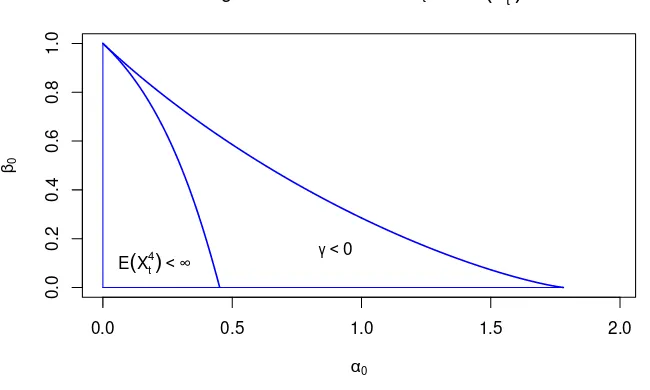
where µn = n!. This condition entails strong restrictions on α0 and β0. The condition for

the existence of a strictly stationary solution to the ACD model isγ :=Elog(α0z1+β0)<0.

Figure 1 shows that the region of strict stationarity is much wider than that of the existence

of fourth-order moments. Under γ < 0, it is know that EXs

t < ∞ for some s > 0, and

thus Elogλk

t <∞ for any k. It follows that QLIK(λ2t) is finite whenever γ < 0, and that QLIK(λt)<_∞ (respectively QLIK(1) <_∞) iff Eλt<_∞ (respectively Eλ2

t <∞).

0.0 0.5 1.0 1.5 2.0

0.0

0.2

0.4

0.6

0.8

1.0

Regions of existence of Xt and E

(

)

α0

β0

γ <0 E(X_t4)< ∞

Figure 1: Region of strict stationarity γ < 0 and region of existence of the fourth-order

moment for the ACD process Xt =λtzt where zt∼Exp(1) and λt=ω0+α0Xt−1+β0λt−1.

5

Numerical illustrations

In this section we first present a small Monte Carlo experiment that compares the finite

sample performance of different estimators of θ0. We then applied our methodology for

predicting a realized volatility series. Other numerical illustrations are available from the

5.1

A simulation study

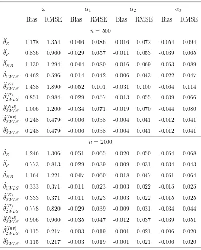
We simulated N = 1000 independent replications of length n = 500 and n = 2000 of

INARCH(q) models, and compared the finite-sample performance of the following estimators:

the PQMLE (1.7), the NBQMLE (1.8) with r=1, the WLSE (1.11) withw_e≡1, and the

two-stage WLS estimators (3.13), (3.14) and (3.15). For choosing between the different versions

of the two-stage WLSE, we used the data-driven methods presented in Section 4. Since the

criterion based of the QLIK loss works much better than that based of the MSE, we only

present the estimator selected by the former (denoted by θb∗

2W LS).

When the cdf is Poisson or Negative Binomial, there is no much difference between

the estimators (thus we do not present these results). Table 1 displays the results for an

INARCH(3) with parameter θ0 = (ω0, α01, α02, α03) = (1,0.3,0.1,0.5), when the cdf is the

Double-Poisson of Efron (1986) of parameters such that the conditional variance iss/λtwith

s = 50.2 _{As expected, the version θ}b(Inv)

2W LS of the two-stage WLSE clearly outperforms the

other estimators, both in terms of bias and Root Mean Square Error (RMSE) of estimation.

Interestingly, the data-chosen WLSE bθ∗

2W LS always coincides with the optimal two-stage

WLSE.

Of course, we made other numerical experiments, that we do not present here to save

space. In particular, we compared the computation time of the different estimators on

INARCH(q) models for increasing values of q. We found that, when the number q + 1

of parameters becomes large the computation time of the QMLEs tends to be prohibitive

because these estimators require numerical optimizations, which is not the case for the WLS

estimators. We also performed Monte Carlo experiments showing that, for all the estimators,

the estimated standard errors based on the asymptotic theory, using the estimators (2.20)

and (2.21), are close to the observed RMSEs on simulations of INGARCH models.

2_{For small values of sthe variance is small and, as a consequence, the weighting sequence wt has little}

Table 1: Bias and RMSE of estimators of the mean parameters when the DGP is a

Double-Poisson INARCH(3).

ω α1 α2 α3

Bias RMSE Bias RMSE Bias RMSE Bias RMSE

n= 500

b

θE 1.178 1.354 -0.046 0.086 -0.016 0.072 -0.054 0.094

b

θP 0.836 0.960 -0.029 0.057 -0.011 0.053 -0.039 0.065

b

θN B 1.130 1.294 -0.044 0.080 -0.016 0.069 -0.053 0.089

b

θ1W LS 0.462 0.596 -0.014 0.042 -0.006 0.043 -0.022 0.047

b

θ₂(E_{W LS}) 1.438 1.890 -0.052 0.101 -0.031 0.100 -0.064 0.114

b

θ₂(P_{W LS}) 0.851 0.984 -0.029 0.057 -0.013 0.055 -0.039 0.066

b

θ₂(N B_{W LS}) 1.006 1.200 -0.034 0.071 -0.019 0.070 -0.044 0.080

b

θ₂(Inv_{W LS}) 0.248 0.479 -0.006 0.038 -0.004 0.041 -0.012 0.041

b

θ∗

2W LS 0.248 0.479 -0.006 0.038 -0.004 0.041 -0.012 0.041

n = 2000

b

θE 1.246 1.306 -0.051 0.065 -0.020 0.050 -0.054 0.068

b

θP 0.773 0.813 -0.029 0.039 -0.009 0.031 -0.034 0.043

b

θN B 1.164 1.221 -0.047 0.060 -0.018 0.047 -0.051 0.064

b

θ1W LS 0.333 0.371 -0.011 0.023 -0.003 0.022 -0.015 0.025

b

θ₂(E_{W LS}) 0.333 0.371 -0.011 0.023 -0.003 0.022 -0.015 0.025

b

θ₂(P_{W LS}) 0.778 0.820 -0.029 0.039 -0.009 0.031 -0.034 0.044

b

θ₂(N B_{W LS}) 0.906 0.960 -0.035 0.047 -0.012 0.037 -0.039 0.051

b

θ₂(Inv_{W LS}) 0.115 0.217 -0.003 0.019 -0.001 0.021 -0.006 0.020

b

θ∗

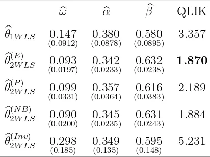
Table 2: WLS estimation results for the CAT series.

b

ω α_b βb QLIK

b

θ1W LS 0.147

(0.0912) (00..0878)380 (00..0895)580 3.357

b

θ(₂E_{W LS}) 0.093

(0.0197) (00..0233)342 (00..0238)632 1.870

b

θ(₂P_{W LS}) 0.099

(0.0331) (00..0364)357 (00..0383)616 2.189

b

θ(₂N B_{W LS}) 0.090

(0.0200) (00..0235)345 (00..0243)631 1.884

b

θ(₂Inv_{W LS}) 0.298

(0.185) 0(0..349135) 0(0..595148) 5.231

5.2

Predicting a realized volatility series

Considerable interest has been paid in recent years to modeling and forecasting daily realized

volatility, which is defined as an integrate variability of high frequency intra-day asset returns

(see e.g. Barndorff-Nielsen and Shephard, 2002). We consider in this subsection the daily

series of Caterpillar Inc. (CAT) realized volatility, from 01/04/1999 to 31/12/2008, which

corresponds to the sample size n = 2489. On this series, we fitted an ACD model with

linear conditional mean (1.2). We found that the first orders p = q = 1 are sufficient

(for larger orders, the usual information criteria AIC and BIC are not smaller, and the

estimated additional parameters are not significantly different from zero). To estimate the

mean parameter of the ACD model, we used the previously described five WLSEs. Table 2

shows that the estimated values of the parameters are close, while their estimated standard

deviations (in parentheses) vary more. The QLIK criterion of Section 4 selects θb₂(E_{W LS}) as the

best WLSE. Note also that bθ(₂E_{W LS}) and θb(₂N B_{W LS}) (now calculated while replacing the estimate

in (3.9) by the value 1) provide almost the same results.

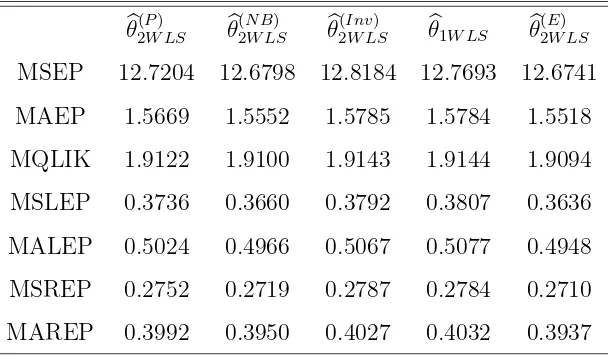
We also compared the performance of the different WLSEs by means of out-of-sample

realized volatility forecast at time t > nc (and horizon 1)

b

Xt=bλt=ωb+ q

X

i=1

b

αiXt−i+ p

X

j=1

b

βjλbt−j

is compared to the actual value Xt, for t = nc + 1, ..., n. We used seven loss functions

considered in Paton (2011): the mean square error prediction, the mean absolute error

prediction, the mean QLIKE, the mean square error prediction, the mean absolute

log-error prediction, the mean square root log-error prediction, and the mean absolute root log-error

prediction, respectively defined by

MSEP = 1

n n

X

t=nc+1

Xt−bλt2, MAEP = 1

n n

X

t=nc+1

Xt−bλt, MQLIK = 1

n n

X

t=nc+1

logbλt+ Xt

b

λt,

MSLEP = 1

n n

X

t=nc+1

logXt−logλtb2, MALEP = 1

n n

X

t=nc+1

logXt−logbλt,

MSREP = 1

n n

X

t=nc+1

p

Xt₋

q b

λt

2

, MAREP = 1

n n

X

t=nc+1

p

Xt₋

q b

λt

2

.

Table 3 displays the loss functions when the learning sample size is nc = 500. Very similar

results have been obtained for nc = 1000 and nc = 1500. Using theR packageMCSdeveloped

by Bernardi and Catania (2014), which implements the Model Confidence Set procedure of

Hansen, Lunde, and Nason (2011), we found that the models estimated byθb(₂E_{W LS}) andθb₂(N B_{W LS})

generally constitute the so-called Superior Set Models. These results comfort those obtained

in-sample: the best estimator is bθ(₂E_{W LS}) , closely followed by θb(₂N B_{W LS}) .

6

Proofs of the main results

Proof of Theorem 2.1 Let Ln(θ, w) and lt(θ, wt) be the random variables obtained by

Table 3: Loss functions for out-of-sample predictions of the CAT realized volatility.

b

θ₂(P_{W LS}) θb(₂N B_{W LS}) θb₂(Inv_{W LS}) θb1W LS θb₂(E_{W LS})

MSEP 12.7204 12.6798 12.8184 12.7693 12.6741

MAEP 1.5669 1.5552 1.5785 1.5784 1.5518

MQLIK 1.9122 1.9100 1.9143 1.9144 1.9094

MSLEP 0.3736 0.3660 0.3792 0.3807 0.3636

MALEP 0.5024 0.4966 0.5067 0.5077 0.4948

MSREP 0.2752 0.2719 0.2787 0.2784 0.2710

MAREP 0.3992 0.3950 0.4027 0.4032 0.3937

without loss of generality that wt ≥w >0. We have

sup

θ∈Θ

lt(θ, wt)₋elt(θ,wt_e)

= sup

θ∈Θ

n e

λt(θ)₋λt(θ)o nλt(θ) +eλt(θ)₋2Xto

e

wt +

(wt−wte){Xt−λt(θ)}2

wtwt_e

≤sup

θ∈Θ

λt(θ)−eλt(θ)

_w2

1 +_|Xt|+ sup θ∈Θ|

λt(θ)|

+_|wt−wet|

2

w2

X_t2+ sup

θ∈Θ

λ2_t(θ)

(6.1)

for t large enough. Therefore, under A2 and A4, by Ces`aro’s lemma we have

sup

θ∈Θ

eLn(θ,w_e)−Ln(θ, w)→0 a.s. as n→ ∞. (6.2)

Now, noting that _{wt, λt(θ), Xt} is a stationary and ergodic process, limn→∞Ln(θ, w) =

Elt(θ, wt)∈[0,∞] a.s. Moreover

Elt(θ0, wt) =E

(Xt−λt)2 wt =E

E

(Xt−λt)2

wt | Ft−1

=Eυt

wt <∞

under A5. Obviously, A3 then implies Elt(θ0, wt)≤ Elt(θ, wt) with equality if and only if

θ =θ0.

The rest of the proof of the consistency (2.3) follows from standard arguments (see e.g.

We now show that the choice of the initial values does not modify the asymptotic

distri-bution of the estimator. Indeed, we have

√

nsup

θ∈Θ

∂Lne (θ,w_e)

∂θ −

∂Ln(θ, w)

∂θ

≤√2

n n X t=1     at w +

|wt−wte|

|Xt|+at+ sup

θ∈Θ|

λt(θ)|

w2

   sup_θ∈Θ

∂λt_∂θ + bt

|Xt|+at+ sup

θ∈Θ|

λt(θ)|

w ,

which tends to zero almost surely, byA8. Now noting that{et,Ft}t, whereet=Xt−λt(θ0),

is a stationary martingale difference sequence, under A6 we have

√

n∂Ln(θ0, w) ∂θ = −2 √ n n X t=1 et wt

∂λt(θ0)

∂θ d

→ N {0,4I(θ0, w)} asn → ∞. (6.3)

Using Taylor expansions and standard arguments (see e.g. the proof of Theorem 2.2 in

Ahmad and Francq, 2016), the convergence in law (2.4) is then proven by showing

∂2_{Ln(θn, w)}

∂θ∂θ′ →2J(θ0, w) as n→ ∞ (6.4)

for any sequenceθn tending toθ0 as n→ ∞. The convergence result (6.4) can be shown by

using the ergodic theorem, the dominated convergence theorem, the continuity of the second

order derivatives of lt(_·, wt) andA7 (see the proof of Theorem 2.2 where, in a more complex

framework, this part of the demonstration is detailed).

Proof of Theorem 2.2 First note that (2.5) entails that for n large enough

|wt,nb ₋wt_{| ≤}Kρt+υ∗

t(ξnb)−υ

∗

t(ξ

∗

0)

≤Kρt+_kξnb ₋ξ∗

0kZt

where Zt= supξ∈V(ξ∗

0)k∂υ

∗

t(ξ)/∂ξk. Therefore, in view of (6.1) and A4

∗

, we have

sup

θ∈Θ