Online Learning in Tensor Space

Online Learning in Tensor Space

Yuan Cao Sanjeev Khudanpur

Center for Language & Speech Processing and Human Language Technology Center of Excellence The Johns Hopkins University

Baltimore, MD, USA, 21218 {yuan.cao, khudanpur}@jhu.edu

Abstract

We propose an online learning algorithm based on space models. A tensor-space model represents data in a compact way, and via rank-1 approximation the weight tensor can be made highly struc-tured, resulting in a significantly smaller number of free parameters to be estimated than in comparable vector-space models. This regularizes the model complexity and makes the tensor model highly effective in situations where a large feature set is de-fined but very limited resources are avail-able for training. We apply with the pro-posed algorithm to a parsing task, and show that even with very little training data the learning algorithm based on a ten-sor model performs well, and gives signif-icantly better results than standard learn-ing algorithms based on traditional vector-space models.

1 Introduction

Many NLP applications use models that try to in-corporate a large number of linguistic features so that as much human knowledge of language can be brought to bear on the (prediction) task as pos-sible. This also makes training the model param-eters a challenging problem, since the amount of labeled training data is usually small compared to the size of feature sets: the feature weights cannot be estimated reliably.

Most traditional models are linear models, in the sense that both the features of the data and model parameters are represented as vectors in a vector space. Many learning algorithms applied to NLP problems, such as the Perceptron (Collins,

2002), MIRA (Crammer et al., 2006; McDonald et al., 2005; Chiang et al., 2008), PRO (Hop-kins and May, 2011), RAMPION (Gimpel and Smith, 2012) etc., are based on vector-space mod-els. Such models require learning individual fea-ture weights directly, so that the number of param-eters to be estimated is identical to the size of the feature set. When millions of features are used but the amount of labeled data is limited, it can be dif-ficult to precisely estimate each feature weight.

In this paper, we shift the model from vector-space to tensor-vector-space. Data can be represented in a compact and structured way using tensors as containers. Tensor representations have been ap-plied to computer vision problems (Hazan et al., 2005; Shashua and Hazan, 2005) and information retrieval (Cai et al., 2006a) a long time ago. More recently, it has also been applied to parsing (Cohen and Collins, 2012; Cohen and Satta, 2013) and se-mantic analysis (Van de Cruys et al., 2013). A linear tensor model represents both features and weights in tensor-space, hence the weight tensor can be factorized and approximated by a linear sum of rank-1 tensors. This low-rank approxi-mation imposes structural constraints on the fea-ture weights and can be regarded as a form of regularization. With this representation, we no longer need to estimate individual feature weights directly but only a small number of “bases” in-stead. This property makes the the tensor model very effective when training a large number of fea-ture weights in a low-resource environment. On the other hand, tensor models have many more de-grees of “design freedom” than vector space mod-els. While this makes them very flexible, it also creates much difficulty in designing an optimal tensor structure for a given training set.

We give detailed description of the tensor space

model in Section 2. Several issues that come with the tensor model construction are addressed in Section 3. A tensor weight learning algorithm is then proposed in 4. Finally we give our exper-imental results on a parsing task and analysis in Section 5.

2 Tensor Space Representation

Most of the learning algorithms for NLP problems are based on vector space models, which represent data as vectors φ ∈ Rn_{, and try to learn feature}

weight vectorsw ∈ Rn _{such that a linear model} y = w·φ is able to discriminate between, say, good and bad hypotheses. While this is a natural way of representing data, it is not the only choice. Below, we reformulate the model from vector to tensor space.

2.1 Tensor Space Model

A tensor is a multidimensional array, and is a gen-eralization of commonly used algebraic objects such as vectors and matrices. Specifically, a vec-tor is a 1st _{order tensor, a matrix is a 2}nd _order

tensor, and data organized as a rectangular cuboid is a 3rd _{order tensor etc. In general, aD}th _order

tensor is represented asT ∈Rn1×n2×...nD, and an

entry inT is denoted byTi1,i2,...,iD. Different

di-mensions of a tensor1,2, . . . , Dare named modes of the tensor.

Using a Dth _{order tensor as container, we can}

assign each feature of the task a D-dimensional index in the tensor and represent the data as ten-sors. Of course, shifting from a vector to a tensor representation entails several additional degrees of freedom, e.g., the order D of the tensor and the sizes {nd}Dd=1 of the modes, which must be

ad-dressed when selecting a tensor model. This will be done in Section 3.

2.2 Tensor Decomposition

Just as a matrix can be decomposed as a lin-ear combination of several rank-1 matrices via SVD, tensors also admit decompositions1_into

lin-ear combinations of “rank-1” tensors. A Dth

or-der tensorA ∈Rn1×n2×...nDis rank-1 if it can be

1_{The form of tensor decomposition defined here is named}

as CANDECOMP/PARAFAC(CP) decomposition (Kolda and Bader, 2009). Another popular form of tensor decom-position is called Tucker decomdecom-position, which decomposes a tensor into a core tensor multiplied by a matrix along each mode. We focus only on the CP decomposition in this paper.

written as the outer product ofDvectors, i.e.

A=a1⊗a2⊗, . . . ,⊗aD,

whereai _∈Rnd,1≤d≤D. ADthorder tensor

T ∈Rn1×n2×...nD can be factorized into a sum of

component rank-1 tensors as

T =XR r=1

Ar= R

X

r=1

a1

r⊗a2r⊗, . . . ,⊗aDr

whereR, called the rank of the tensor, is the mini-mum number of rank-1 tensors whose sum equals

T. Via decomposition, one may approximate a tensor by the sum ofHmajor rank-1 tensors with

H≤R.

2.3 Linear Tensor Model

In tensor space, a linear model may be written (ig-noring a bias term) as

f(W) =W ◦Φ,

whereΦ∈Rn1×n2×...nDis the feature tensor,W

is the corresponding weight tensor, and◦denotes the Hadamard product. If W is further decom-posed as the sum ofH major component rank-1 tensors, i.e. W ≈PH_h=1w1

h⊗w2h⊗, . . . ,⊗wDh,

then

f(w1

1, . . . ,wD1 , . . . ,w1h, . . . ,wDh) = XH

h=1

Φ×1w1h×2w2h. . .×DwDh, (1)

where×l is thel-mode product operator between

aDth_{order tensorT and a vectoraof dimension}

nd, yielding a(D−1)thorder tensor such that

(T ×la)i1,...,il−1,il+1,...,iD

= Xnd il=1

Ti1,...,il−1,il,il+1,...,iD ·ail.

The linear tensor model is illustrated in Figure 1.

2.4 Why Learning in Tensor Space?

So what is the advantage of learning with a ten-sor model instead of a vector model? Consider the case where we have defined 1,000,000 features for our task. A vector space linear model requires es-timating 1,000,000 free parameters. However if we use a2nd_{order tensor model, organize the}

Figure 1: A 3rd _{order linear tensor model. The}

feature weight tensor W can be decomposed as the sum of a sequence of rank-1 component ten-sors.

one rank-1 matrix to approximate the weight ten-sor, then the linear model becomes

f(w1,w2) =wT1Φw2,

where w1,w2 ∈ R1000. That is to say, now we

only need to estimate 2000 parameters!

In general, ifV features are defined for a learn-ing problem, and we (i) organize the feature set as a tensor Φ ∈ Rn1×n2×...nD and (ii) use H

component rank-1 tensors to approximate the cor-responding target weight tensor. Then the total number of parameters to be learned for this ten-sor model isHPD_d=1nd, which is usually much

smaller thanV = QD_d=1ndfor a traditional

vec-tor space model. Therefore we expect the tensor model to be more effective in a low-resource train-ing environment.

Specifically, a vector space model assumes each feature weight to be a “free” parameter, and es-timating them reliably could therefore be hard when training data are not sufficient or the fea-ture set is huge. By contrast, a linear tensor model only needs to learnHPD_d=1nd “bases” of them

feature weights instead of individual weights di-rectly. The weight corresponding to the feature

Φi1,i2,...,iD in the tensor model is expressed as

wi1,i2,...,iD =

H

X

h=1

w_h,i1 ₁w_h,i2 ₂. . . w_h,iD_D, (2)

wherewj_h,ij is theith

j element in the vectorwjh.

In other words, a true feature weight is now ap-proximated by a set of bases. This reminds us of the well-known low-rank matrix approximation of images via SVD, and we are applying similar techniques to approximate target feature weights, which is made possible only after we shift from vector to tensor space models.

This approximation can be treated as a form of model regularization, since the weight tensor is represented in a constrained form and made highly structured via the rank-1 tensor approximation. Of course, as we reduce the model complexity, e.g. by choosing a smaller and smallerH, the model’s ex-pressive ability is weakened at the same time. We will elaborate on this point in Section 3.1.

3 Tensor Model Construction

To apply a tensor model, we first need to con-vert the feature vector into a tensorΦ. Once the structure ofΦis determined, the structure of W is fixed as well. As mentioned in Section 2.1, a tensor model has many more degrees of “design freedom” than a vector model, which makes the problem of finding a good tensor structure a non-trivial one.

3.1 Tensor Order

The order of a tensor affects the model in two ways: the expressiveness of the model and the number of parameters to be estimated. We assume

H = 1in the analysis below, noting that one can always add as many rank-1 component tensors as needed to approximate a tensor with arbitrary pre-cision.

Obviously, the 1st _{order tensor (vector) model}

is the most expressive, since it is structureless and any arbitrary set of numbers can always be repre-sented exactly as a vector. The2nd _{order rank-1}

tensor (rank-1 matrix) is less expressive because not every set of numbers can be organized into a rank-1 matrix. In general, a Dth _{order rank-1}

tensor is more expressive than a(D+ 1)th _order

rank-1 tensor, as a lower-order tensor imposes less structural constraints on the set of numbers it can express. We formally state this fact as follows:

Theorem 1. A set of real numbers that can be rep-resented by a(D+ 1)th _{order tensorQ can also}

be represented by aDth_{order tensorP, provided}

P andQhave the same volume. But the reverse is not true.

Proof. See appendix.

On the other hand, tensor order also affects the number of parameters to be trained. Assuming that aDth_{order has equal size on each mode (we}

of the model is DVD1. This is a convex

func-tion ofD, and the minimum2 _{is reached at either} D∗ _=blnVcorD∗_=dlnVe.

Therefore, as D increases from 1 to D∗_{, we}

lose more and more of the expressive power of the model but reduce the number of parameters to be trained. However it would be a bad idea to choose aDbeyondD∗_{. The optimal tensor order depends}

on the nature of the actual problem, and we tune this hyper-parameter on a held-out set.

3.2 Mode Size

The size nd of each tensor mode, d = 1, . . . , D,

determines the structure of feature weights a ten-sor model can precisely represent, as well as the number of parameters to estimate (we also as-sumeH = 1 in the analysis below). For exam-ple, if the tensor order is 2 and the volume V is 12, then we can either choose n1 = 3, n2 = 4

or n1 = 2, n2 = 6. For n1 = 3, n2 = 4, the

numbers that can be precisely represented are di-vided into 3 groups, each having 4 numbers, that are scaled versions of one another. Similarly for

n1 = 2, n2 = 6, the numbers can be divided into

2 groups with different scales. Obviously, the two possible choices of(n1, n2)also lead to different

numbers of free parameters (7 vs. 8).

GivenDandV, there are many possible combi-nations ofnd, d= 1, . . . , D, and the optimal

com-bination should indeed be determined by the struc-ture of target feastruc-tures weights. However it is hard to know the structure of target feature weights be-fore learning, and it would be impractical to try ev-ery possible combination of mode sizes, therefore we choose the criterion of determining the mode sizes as minimization of the total number of pa-rameters, namely we solve the problem:

min n1,...,nD

D

X

d=1

nd s.t D

Y

d=1

nd=V

The optimal solution is reached whenn1 =n2 =

. . . = nD = VD1. Of course it is not

guaran-teed that VD1 is an integer, therefore we choose

nd = bVD1c or dVD1e, d = 1, . . . , D such that

Q_D

d=1nd≥V andhQDd=1nd

i

−V is minimized. The hQD_d=1nd

i

− V extra entries of the tensor correspond to no features and are used just for 2_{The optimal integer solution can be determined simply}

by comparing the two function values.

padding. Since for each nd there are only two

possible values to choose, we can simply enumer-ate all the possible2D _{(which is usually a small}

number) combinations of values and pick the one that matches the conditions given above. This way

n1, . . . , nD are fully determined.

Here we are only following the principle of min-imizing the parameter number. While this strat-egy might work well with small amount of train-ing data, it is not guaranteed to be the best strategy in all cases, especially when more data is avail-able we might want to increase the number of pa-rameters, making the model more complex so that the data can be more precisely modeled. Ideally the mode size needs to be adaptive to the amount of training data as well as the property of target weights. A theoretically guaranteed optimal ap-proach to determining the mode sizes remains an open problem, and will be explored in our future work.

3.3 Number of Rank-1 Tensors

The impact of usingH > 1rank-1 tensors is ob-vious: a largerHincreases the model complexity and makes the model more expressive, since we are able to approximate target weight tensor with smaller error. As a trade-off, the number of param-eters and training complexity will be increased. To find out the optimal value ofH for a given prob-lem, we tune this hyper-parameter too on a held-out set.

3.4 Vector to Tensor Mapping

Finally, we need to find a way to map the orig-inal feature vector to a tensor, i.e. to associate each feature with an index in the tensor. Assum-ing the tensor volumeV is the same as the number of features, then there are in allV!ways of map-ping, which is an intractable number of possibili-ties even for modest sized feature sets, making it impractical to carry out a brute force search. How-ever while we are doing the mapping, we hope to arrange the features in a way such that the corre-sponding target weight tensor has approximately a low-rank structure, this way it can be well approx-imated by very few component rank-1 tensors.

“surro-gate” weight vector. We then use this surrogate vector to guide the design of the mapping. Ide-ally we hope to find a permutation of the surro-gate weights to map to a tensor in such a way that the tensor has a rank as low as possible. How-ever matrix rank minimization is in general a hard problem (Fazel, 2002). Therefore, we follow an approximate algorithm given in Figure 2a, whose main idea is illustrated via an example in Figure 2b.

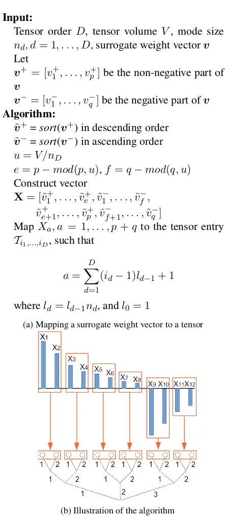
Basically, what the algorithm does is to di-vide the surrogate weights into hierarchical groups such that groups on the same level are approx-imately proportional to each other. Using these groups as units we are able to “fill” the tensor in a hierarchical way. The resulting tensor will have an approximate low-rank structure, provided that the sorted feature weights have roughly group-wise proportional relations.

For comparison, we also experimented a trivial solution which maps each entry of the feature ten-sor to the tenten-sor just in sequential order, namely

φ0is mapped toΦ0,0,...,0,φ1is mapped toΦ0,0,...,1

etc. This of course ignores correlation between features since the original feature order in the vec-tor could be totally meaningless, and this strategy is not expected to be a good solution for vector to tensor mapping.

4 Online Learning Algorithm

We now turn to the problem of learning the feature weight tensor. Here we propose an online learning algorithm similar to MIRA but modified to accom-modate tensor models.

Let the model bef(T) = T ◦Φ(x, y), where T = PH_h=1w1

h ⊗w2h⊗, . . . ,⊗wDh is the weight

tensor, Φ(x, y) is the feature tensor for an input-output pair(x, y). Training samples (xi, yi), i = 1, . . . , m, wherexi is the input and yi is the ref-erence or oracle hypothesis, are fed to the weight learning algorithm in sequential order. A predic-tion zt is made by the model Tt at time tfrom a set of candidatesZ(xt), and the model updates the

weight tensor by solving the following problem:

min

T∈Rn1×n2×...nD

1

2kT −Ttk2+Cξ (3) s.t.

Lt≤ξ, ξ≥0

whereT is a decomposed weight tensor and

Lt=T ◦Φ(xt, zt)−T ◦Φ(xt, yt) +ρ(yt, zt)

Input:

Tensor order D, tensor volume V, mode size

nd, d= 1, . . . , D, surrogate weight vectorv

Let v+ _{= [v}+

1, . . . , vp+]be the non-negative part of

v

v−_{= [v}−

1, . . . , vq−]be the negative part ofv Algorithm:

˜

v+_=sort(v+_{) in descending order}

˜

v−_=sort(v−_{) in ascending order}

u=V/nD

e=p−mod(p, u),f =q−mod(q, u)

Construct vector

X= [˜v₁+, . . . ,˜v+

e,v˜1−, . . . ,˜v−f, ˜

v_e+₊₁, . . . ,˜v+

p,v˜f−+1, . . . ,˜v−q]

MapXa, a = 1, . . . , p+q to the tensor entry Ti1,...,iD, such that

a= D

X

d=1

(id−1)ld−1+ 1

whereld=ld−1nd, andl0 = 1

(a) Mapping a surrogate weight vector to a tensor

(b) Illustration of the algorithm

Figure 2: Algorithm for mapping a surrogate weight vectorX to a tensor. (2a) provides the al-gorithm; (2b) illustrates it by mapping a vector of lengthV = 12to a (n1, n2, n3) = (2,2,3)

is the structured hinge loss.

This problem setting follows the same “passive-aggressive” strategy as in the original MIRA. To optimize the vectors wd

h, h = 1, . . . , H, d = 1, . . . , D, we use a similar iterative strategy as pro-posed in (Cai et al., 2006b). Basically, the idea is that instead of optimizingwd

h all together, we

op-timizew1

1,w21, . . . ,wDH in turn. While we are

up-dating one vector, the rest are fixed. For the prob-lem setting given above, each of the sub-probprob-lems that need to be solved is convex, and according to (Cai et al., 2006b) the objective function value will decrease after each individual weight update and eventually this procedure will converge.

We now give this procedure in more detail. Denote the weight vector of the dth _{mode of}

the hth _{tensor at time t as w}d

h,t. We will

up-date the vectors in turn in the following order: w1

1,t, . . . ,wD1,t,w12,t, . . . ,wD2,t, . . . ,w1H,t, . . . ,wDH,t.

Once a vector has been updated, it is fixed for future updates.

By way of notation, define

Wd

h,t = w1

h,t+1⊗, . . . ,⊗wdh,t−1+1⊗wdh,t⊗, . . . ,⊗wDh,t

(and letWD_h,t+1,w1_h,t+1⊗, . . . ,⊗wD_h,t+1),

c

Wd_h,t

= w1_h,t+1⊗, . . . ,⊗w_h,td−1₊₁⊗wd⊗, . . . ,⊗wD_h,t (wherewd_∈Rnd),

Td_h,t = h−1

X

h0₌₁

WD_h0+1_,t +Wd_h,t+

H

X

h0_=h+1

W1_h0_,t(4)

b

Td_h,t = hX−1 h0₌₁

WD_h0+1_,t +Wcd_h,t+

H

X

h0_=h+1 W1_h0_,t

φd_h,t(x, y)

= Φ(x, y)×2w2h,t+1. . .×d−1wdh,t−1+1×d+1 wd_h,t+1. . .×DwD_h,t (5)

In order to update from wd

h,t to get wdh,t+1, the

sub-problem to solve is:

min

wd∈Rnd

1 2kTb

d

h,t−Tdh,tk2+Cξ

= min

wd∈Rnd

1 2kWc

d

h,t−Wdh,tk2+Cξ

= min

wd∈Rnd

1

2βh,t1 +1. . . βh,td−1+1βh,td+1. . . βh,tD kwd_−wd

h,tk2+Cξ s.t. L_h,td ≤ξ, ξ ≥0.

where

βd

h,t = kwdh,tk2

Ld

h,t = Tbdh,t◦Φ(xt, zt)−Tbdh,t◦Φ(xt, yt) +ρ(yt, zt)

= wd·φd_h,t(xt, zt)−φd_h,t(xt, yt)

− hX−1 h0₌₁

WD_h0+1_,t +

H

X

h0_=h+1 W1_h0_,t

!

◦

(Φ(xt, yt)−Φ(xt, zt)) +ρ(yt, zt)

Letting

∆φd

h,t,φdh,t(xt, yt)−φdh,t(xt, zt)

and

sd_h,t ,

h−1

X

h0₌₁

WD_h0+1_,t +

H

X

h0_=h+1 W1_h0_,t

!

◦

(Φ(xt, yt)−Φ(xt, zt))

we may compactly write

Ld

h,t =ρ(yt, zt)−sdh,t−wd·∆φdh,t.

This convex optimization problem is just like the original MIRA and may be solved in a similar way. The updating strategy forwd

h,tis derived as

wd

h,t+1 =wdh,t+τ∆φdh,t

τ = (6)

min

(

C,ρ(yt, zt)−Tdh,t◦(Φ(xt, yt)−Φ(xt, zt)) k∆φd_h,tk2

)

The initial vectorswi

h,1 cannot be made all zero,

since otherwise the l-mode product in Equation (5) would yield all zeroφd

h,t(x, y) and the model

would never get a chance to be updated. There-fore, we initialize the entries of wi

h,1 uniformly

such that the Frobenius-norm of the weight tensor W is unity.

5 Experiments

In this section we shows empirical results of the training algorithm on a parsing task. We used the Charniak parser (Charniak et al., 2005) for our ex-periment, and we used the proposed algorithm to train the reranking feature weights. For compari-son, we also investigated training the reranker with Perceptron and MIRA.

5.1 Experimental Settings

To simulate a low-resource training environment, our training sets were selected from sections 2-9 of the Penn WSJ treebank, section 24 was used as the held-out set and section 23 as the evaluation set. We applied the default settings of the parser. There are around V = 1.33 million features in all defined for reranking, and the n-best size for reranking is set to 50. We selected the parse with the highestf-score from the 50-best list as the or-acle.

We would like to observe from the experiments how the amount of training data as well as dif-ferent settings of the tensor degrees of freedom affects the algorithm performance. Therefore we tried all combinations of the following experimen-tal parameters:

Parameters Settings

Training data (m) Sec. 2, 2-3, 2-5, 2-9 Tensor order (D) 2, 3, 4 # rank-1 tensors (H) 1, 2, 3

Vec. to tensor mapping approximate, sequential

Here “approximate” and “sequential” means us-ing, respectively, the algorithm given in Figure 2 and the sequential mapping mentioned in Section 3.4. According to the strategy given in 3.2, once the tensor order and number of features are fixed, the sizes of modes and total number of parameters to estimate are fixed as well, as shown in the tables below:

D Size of modes Number of parameters

2 1155×1155 2310

3 110×110×111 331

4 34×34×34×34 136

5.2 Results and Analysis

The f-scores of the held-out and evaluation set given by T-MIRA as well as the Perceptron and

MIRA baseline are given in Table 1. From the re-sults, we have the following observations:

1. When very few labeled data are available for training (compared with the number of fea-tures), T-MIRA performs much better than the vector-based models MIRA and Percep-tron. However as the amount of training data increases, the advantage of T-MIRA fades away, and vector-based models catch up. This is because the weight tensors learned by T-MIRA are highly structured, which sig-nificantly reduces model/training complex-ity and makes the learning process very ef-fective in a low-resource environment, but as the amount of data increases, the more complex and expressive vector-based models adapt to the data better, whereas further im-provements from the tensor model is impeded by its structural constraints, making it insen-sitive to the increase of training data.

2. To further contrast the behavior of T-MIRA, MIRA and Perceptron, we plot thef-scores on both the training and held-out sets given by these algorithms after each training epoch in Figure 3. The plots are for the exper-imental setting with mapping=surrogate, # rank-1 tensors=2, tensor order=2, training data=sections 2-3. It is clearly seen that both MIRA and Perceptron do much better than T-MIRA on the training set. Nevertheless, with a huge number of parameters to fit a limited amount of data, they tend to over-fit and give much worse results on the held-out set than T-MIRA does.

As an aside, observe that MIRA consistently outperformed Perceptron, as expected. 3. Properties of linear tensor model: The

heuris-tic vector-to-tensor mapping strategy given by Figure 2 gives consistently better results than the sequential mapping strategy, as ex-pected.

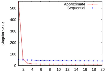
To make further comparison of the two strate-gies, in Figure 4 we plot the 20 largest sin-gular values of the matrices which the surro-gate weights (given by the Perceptron after running for 1 epoch) are mapped to by both strategies (from the experiment with training data sections 2-5). From the contrast between the largest and the 2nd_{-largest singular}

by the first strategy approximates a low-rank structure much better than the second strat-egy. Therefore, the performance of T-MIRA is influenced significantly by the way features are mapped to the tensor. If the correspond-ing target weight tensor has internal struc-ture that makes it approximately low-rank, the learning procedure becomes more effec-tive.

The best results are consistently given by2nd

order tensor models, and the differences be-tween the 3rd _{and 4}th _{order tensors are not}

significant. As discussed in Section 3.1, al-though3rd_and4th_{order tensors have less}

pa-rameters, the benefit of reduced training com-plexity does not compensate for the loss of expressiveness. A 2nd _{order tensor has}

al-ready reduced the number of parameters from the original 1.33 million to only 2310, and it does not help to further reduce the number of parameters using higher order tensors. 4. As the amount of training data increases,

there is a trend that the best results come from models with more rank-1 component tensors. Adding more rank-1 tensors increases the model’s complexity and ability of expression, making the model more adaptive to larger data sets.

6 Conclusion and Future Work

In this paper, we reformulated the traditional lin-ear vector-space models as tensor-space models, and proposed an online learning algorithm named Tensor-MIRA. A tensor-space model is a com-pact representation of data, and via rank-1 ten-sor approximation, the weight tenten-sor can be made highly structured hence the number of parame-ters to be trained is significantly reduced. This can be regarded as a form of model regular-ization.Therefore, compared with the traditional vector-space models, learning in the tensor space is very effective when a large feature set is defined, but only small amount of training data is available. Our experimental results corroborated this argu-ment.

As mentioned in Section 3.2, one interesting problem that merits further investigation is how to determine optimal mode sizes. The challenge of applying a tensor model comes from finding a proper tensor structure for a given problem, and

95.5 96 96.5 97 97.5 98 98.5 99

1 2 3 4 5 6 7 8 9 10

f-score

Iterations Training set f-score

T-MIRA MIRA Perceptron

(a) Training set

87 87.5 88 88.5 89 89.5 90

1 2 3 4 5 6 7 8 9 10

f-score

Iterations Training set f-score

T-MIRA MIRA Perceptron

(b) Held-out set

Figure 3: f-scores given by three algorithms on training and held-out set (see text for the setting).

the key to solving this problem is to find a bal-ance between the model complexity (indicated by the order and sizes of modes) and the number of parameters. Developing a theoretically guaran-teed approach of finding the optimal structure for a given task will make the tensor model not only perform well in low-resource environments, but adaptive to larger data sets.

7 Acknowledgements

This work was partially supported by IBM via DARPA/BOLT contract number HR0011-12-C-0015 and by the National Science Foundation via award number IIS-0963898.

References

Deng Cai , Xiaofei He , and Jiawei Han. 2006. Tensor Space Model for Document Analysis Proceedings of the 29th Annual International ACM SIGIR Con-ference on Research and Development in Informa-tion Retrieval(SIGIR), 625–626.

Mapping Approximate Sequential

Rank-1 tensors 1 2 3 1 2 3

Tensor order 2 3 4 2 3 4 2 3 4 2 3 4 2 3 4 2 3 4

Held-out score 89.43 89.16 89.22 89.16 89.21 89.24 89.27 89.14 89.24 89.21 88.90 88.89 89.13 88.88 88.88 89.15 88.87 88.99

Evaluation score 89.83 89.69

MIRA 88.57

Percep 88.23

(a) Training data: Section 2 only

Mapping Approximate Sequential

Rank-1 tensors 1 2 3 1 2 3

Tensor order 2 3 4 2 3 4 2 3 4 2 3 4 2 3 4 2 3 4

Held-out score 89.26 89.06 89.12 89.33 89.11 89.19 89.18 89.14 89.15 89.2 89.01 88.82 89.24 88.94 88.95 89.19 88.91 88.98

Evaluation score 90.02 89.82

MIRA 89.00

Percep 88.59

(b) Training data: Section 2-3

Mapping Approximate Sequential

Rank-1 tensors 1 2 3 1 2 3

Tensor order 2 3 4 2 3 4 2 3 4 2 3 4 2 3 4 2 3 4

Held-out score 89.40 89.44 89.17 89.5 89.37 89.18 89.47 89.32 89.18 89.23 89.03 88.93 89.24 88.98 88.94 89.16 89.01 88.85

Evaluation score 89.96 89.78

MIRA 89.49

Percep 89.10

(c) Training data: Section 2-5

Mapping Approximate Sequential

Rank-1 tensors 2 3 4 2 3 4

Tensor order 2 3 4 2 3 4 2 3 4 2 3 4 2 3 4 2 3 4

Held-out score 89.43 89.23 89.06 89.37 89.23 89.1 89.44 89.22 89.06 89.21 88.92 88.94 89.23 88.94 88.93 89.23 88.95 88.93

Evaluation score 89.95 89.84

MIRA 89.95

Percep 89.77

(d) Training data: Section 2-9

Table 1: Parsingf-scores. Tables (a) to (d) correspond to training data with increasing size. The upper-part of each table shows the T-MIRA results with different settings, the lower-part shows the MIRA and Perceptron baselines. The evaluation scores come from the settings indicated by the best held-out scores. The best results on the held-out and evaluation data are marked in bold.

0 100 200 300 400 500

2 4 6 8 10 12 14 16 18 20

Singular value

Approximate Sequential

Figure 4: The top 20 singular values of the surro-gate weight matrices given by two mapping algo-rithms.

Eugene Charniak, and Mark Johnson 2005. Coarse-to-fine n-Best Parsing and MaxEnt Discriminative Reranking Proceedings of the 43th Annual Meeting on Association for Computational Linguistics(ACL)

173–180.

David Chiang, Yuval Marton, and Philip Resnik. 2008. Online Large-Margin Training of Syntactic and Structural Translation Features Proceedings of Empirical Methods in Natural Language

Process-ing(EMNLP), 224–233.

Shay Cohen and Michael Collins. 2012. Tensor De-composition for Fast Parsing with Latent-Variable PCFGs Proceedings of Advances in Neural Infor-mation Processing Systems(NIPS).

Shay Cohen and Giorgio Satta. 2013. Approximate PCFG Parsing Using Tensor Decomposition Pro-ceedings of NAACL-HLT, 487–496.

Michael Collins. 2002. Discriminative training meth-ods for hidden Markov Models: Theory and Exper-iments with Perceptron. Algorithms Proceedings of Empirical Methods in Natural Language Process-ing(EMNLP), 10:1–8.

Koby Crammer, Ofer Dekel, Joseph Keshet, Shai Shalev-Schwartz, and Yoram Singer. 2006. Online Passive-Aggressive Algorithms Journal of Machine Learning Research(JMLR), 7:551–585.

Maryam Fazel. 2002. Matrix Rank Minimization with Applications PhD thesis, Stanford University. Kevin Gimpel, and Noah A. Smith 2012. Structured

Ramp Loss Minimization for Machine Translation

Tamir Hazan, Simon Polak, and Amnon Shashua 2005. Sparse Image Coding using a 3D Non-negative Ten-sor Factorization Proceedings of the International Conference on Computer Vision (ICCV).

Mark Hopkins and Jonathan May. 2011. Tuning as Reranking Proceedings of Empirical Methods in Natural Language Processing(EMNLP), 1352-1362.

Tamara Kolda and Brett Bader. 2009. Tensor Decom-positions and Applications SIAM Review, 51:455-550.

Ryan McDonald, Koby Crammer, and Fernando Pereira. 2005. Online Large-Margin Training of Dependency Parsers Proceedings of the 43rd An-nual Meeting of the ACL, 91–98.

Amnon Shashua, and Tamir Hazan. 2005. Non-Negative Tensor Factorization with Applications to Statistics and Computer Vision Proceedings of the International Conference on Machine Learning (ICML).

Tim Van de Cruys, Thierry Poibeau, and Anna Korho-nen. 2013. A Tensor-based Factorization Model of Semantic Compositionality Proceedings of NAACL-HLT, 1142–1151.

A Proof of Theorem 1

Proof. For D = 1, it is obvious that if a set of real numbers{x1, . . . , xn}can be represented by

a rank-1 matrix, it can always be represented by a vector, but the reverse is not true.

For D > 1, if {x1, . . . , xn} can be

repre-sented by P = p1 ⊗ p2 ⊗ . . . ⊗pD, namely xi = Pi1,...,iD =

Q_D

d=1pdid, then for any

compo-nent vector in moded,

[pd₁, pd₂, . . . , pd_nd] = [s₁dpd₁, sd₂pd₁, . . . , sd_np dp

d

1]

wherenp_dis the size of modedofP,sd

j is a

con-stant andsd

j = ppii11_,...,id,...,id−₋1₁,j,id,1_,id+1₊₁,...,iD_,...,iD Therefore

xi=Pi1,...,iD =x1,...,1

D

Y

d=1

sd_id (7)

and this representation is unique for a givenD(up to the ordering ofpj andsdj inpj, which simply

assigns{x1, . . . , xn}with different indices in the

tensor), due to the pairwise proportional constraint imposed byxi/xj, i, j= 1, . . . , n.

If xi can also be represented byQ, thenxi = Qi1,...,iD+1 = x1,...,1

Q_D+1

d=1 tdid, where tdj has a

similar definition assd

j. Then it must be the case

that

∃d1, d2 ∈ {1, . . . , D+ 1}, d∈ {1, . . . , D}, d1 6=d2

s.t. td1

id₁t

d2

id₂ =s

d

id, (8)

tda

ida =s

db

i_db, da6=d1, d2, db 6=d

since otherwise {x1, . . . , xn} would be

repre-sented by a different set of factors than those given in Equation (7).

Therefore, in order for tensor Q to represent the same set of real numbers that P represents, there needs to exist a vector[sd

1, . . . , sdnd]that can

be represented by a rank-1 matrix as indicated by Equation (8), which is in general not guaranteed.

On the other hand, if{x1, . . . , xn}can be

rep-resented byQ, namely

xi =Qi1,...,iD+1 =

D_Y+1

d=1

qd_id

then we can just pickd1 ∈ {1, . . . , D}, d2 =d1+

1and let

q0 _{= [q}d1

1 q1d2, qd11q2d2, . . . , qnd1q_d2qdn2q_d1]

and

Q0 =q1⊗. . .⊗qd1−1⊗q0⊗qd2+1⊗. . .⊗qD+1

Hence{x1, . . . , xn}can also be represented by a