Zero-shot Recognition via Direct Classifier Learning
with Transferred Samples and Pseudo Labels
AAAI Anonymous Submission 182
Abstract
As an interesting and emerging topic, zero-shot recognition (ZSR) makes it possible to train a recognition model by spec-ifying the category’s attributes when there are no labeled ex-emplars available. The fundamental idea for ZSR is to trans-fer knowledge from the abundant labeled data in diftrans-ferent but related source classes via the class attributes. Conventional ZSR approaches adopt atwo-stepstrategy in test stage, where the samples are projected into the attribute space in the first step, and then the recognition is carried out based on consid-ering the relationship between samples and classes in the at-tribute space. Due to this intermediate transformation, infor-mation loss is unavoidable, thus degrading the performance of the overall system. Rather than following this two-step s-trategy, in this paper, we propose a novelone-stepapproach that is able to perform ZSR in the original feature space by using directly trained classifiers. To tackle the problem that no labeled samples of target classes are available, we propose to assignpseudo labelsto samples based on the reliability and diversity, which in turn will be used to train the classi-fiers. Moreover, we adopt a robust SVM that accounts for the unreliability of pseudo labels. Extensive experiments on four datasets demonstrate consistent performance gains of our ap-proach over the state-of-the-art two-step ZSR apap-proaches.
Introduction
In the recent years, we have witnessed the emerging of zero-shot recognition (ZSR) in computer vision and related com-munities. Basically, the objective of ZSR is to build classi-fication models for target classes with no labeled samples (Lampert, Nickisch, and Harmeling 2014). To construct su-pervised models without supervision information for target classes, existing approaches make use of knowledge from related but different source classes which are well labeled, and transfer the knowledge to target classes via the classes’ attributes (Farhadi et al. 2009; Socher et al. 2013). Gener-ally, a two-step strategy in the test stage is adopted. First-ly, based on the supervision information in source classes, a projection function that projects the original features into the attribute space is learned, such as linear projection (Akata et al. 2013) and n-way classifier (Norouzi et al. 2013). Sec-ondly, after projecting a test sample from the target classes
Copyright c2017, Association for the Advancement of Artificial Intelligence (www.aaai.org). All rights reserved.
Dog
Cat
Car Truck
Source Class Target Class
Car
Cat Truck
Class Attributes
Attribute Space
Car Dog
Cat
Truck
Projection
0.13 0.88
Car Dog
Sample Selection & Pseudo Label
Classifier Prediction
Original Space Dog
[image:1.612.328.552.220.445.2]Car
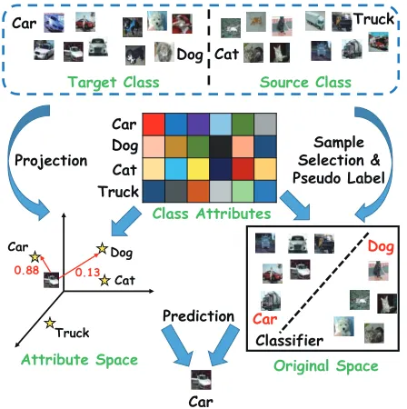
Figure 1: Frameworks of the previous two-step strategy and the proposed one-step approach. Ours does not require the intermediate space in theteststage while the previous do.
into the attribute space, the classification is performed by considering the relationship between the test sample and all target classes in the attribute space. Typically, the relation-ship can be measured by Euclidean distance (Socher et al. 2013), inner-product similarity (Guo et al. 2016), and man-ifold distance (Fu et al. 2015). The basic framework of the two-step strategy is illustrated in Figure 1 on the left side.
In this paper, we propose a novel approach that adopts
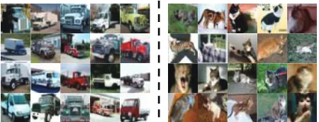
Figure 2: Some selected sample images from truck and cat. We use them with pseudo labels to train a car-dog classifier.
labeled samples from truck and cat. Intuitively, we can se-lect some samples from truck class alike to car (measured in the attribute space) and treat them as the labeled samples for car. Similarly, we can select some samples from cat as the labeled samples for dog. Having used the pseudo labels, a classifier can be trained as usual. It is believed that such a scheme is very logical because human being often uses one category to deduce another one as long as they share the same characteristics. In Figure 2, we illustrate20 selected images (500in total) from truck and cat respectively. We as-sign pseudo labels to them, and on top of it, we train a linear car-dog SVM classifier. We found out that the classifier is able to achieve92.80%recognition accuracy in the test set.
Implementing the above idea in a ZSR system is not that simple, because we have to solve two problems. Firstly, we need to select proper samples for pseudo labeling. Here, we take two aspects into consideration for the sample selection procedure, which are reliability and diversity. The former reflects how a sample is similar to the target classes while the latter one shows how the selected samples cover the d-ifferent characteristics of target classes. In our approach, we formulate them as a joint quadratic problem. Secondly, we have to deal with the label noise which arises from the fact that the pseudo labels are not the true labels. To alleviate the influence of the label noise, we propose to use a robust SVM classifier. The main contributions of this paper are as below:
• We propose a novel one-step approach for ZSR. Classi-fiers for target classes are directly trained in the original feature space by using the pseudo labels. Such classifiers allow to directly predict the class labels from test samples without utilizing the attribute space as the intermediary so that less information is leaked in the whole procedure.
• To select good samples for pseudo labeling, we propose a quadratic formulation taking into account the reliability and the diversity of the selected samples simultaneously.
• To cope with the label noise existed in the pseudo labels, we make use of a robust SVM as the classifier which can be derived from the standard SVM and efficiently trained.
Related Work
Now we introduce the key principles for ZSR and ZSR varia-tions. For ease of explanation, we firstly define the notavaria-tions.
Notations
We have a set of source classesCs = {cs
1, ..., csks} andns labeled source samples Ds = {(xs
1,ys1), ...,(xsns,y s ns)},
Table 1: Notations and descriptions.
Notation Description Notation Description
xs,xt features ns, nt #samples
ys,yt label vector d #dimension
as,at class attribute q #attributes
α weights ks, kt #classes
r ranking score σ, β, µ, C parameters
wherexs
i ∈ Rdis the feature vector andyis ∈ {0,1}ks is the corresponding label vector which hasyij= 1if the sam-pleibelongs to classcs
j or0otherwise. We are given some target samples Dt = {xt
1, ...,xtnt} from kt target classes
Ct={ct
1, ..., ctkt}satisfyingC
s∩ Ct=∅. The goal of ZSR is to build classification models which can predict the label
c(xt
i)givenxtiwith no labeled training data for target class-es. For each classci ∈ Cs∪ Ct, we assign a class attribute representationai ∈Rq to it. We summarize some notations in this paper and the corresponding descriptions in Table 1.
Basic Idea of ZSR
Generally, the classification in ZSR can be summarized as:
c(xti) =argmaxc∈Ctsim(ac,P(xti)), (1)
where sim(·,·)denotes a similarity / distance measure, and
Prepresents a projection function which is learned as below,
P =argminP
ns
X
i=1
ℓ(P(xsi),ac(xs
i)), (2)
whereℓ(·,·)is a loss function. As the source samples are ful-ly labeled,c(xsi)is known for the above problem. And since the attributes are shared among source and target classes, the projection learned based on the source classes also works in the target classes (Lampert, Nickisch, and Harmeling 2014).
ZSR Variations
The main difference of various ZSR approaches lies in using different projections or/and similarity measures. Lampert et al. (2009) propose Direct Attribute Prediction which adopt-s binary claadopt-sadopt-sifieradopt-s for P and Euclidean distance. Socher et al. (2013) propose a Cross-modal Transfer which uses a nonlinear projection forP and isometric Gaussian probabil-ity. Akata et al. (2013) propose a Label Embedding which adopts a linear projection and Euclidean distance. Fu et al. (2015) propose to use a deep model DeViSE (Frome et al. 2013) for projection and measure the similarity using the se-mantic manifold distance obtained from absorbing Markov chain process. Jayaraman and Grauman (2014) propose a random forest approach and the prediction error statistics of attributes are considered in the similarity measure. Kodirov et al. (2015) propose to use sparse coding for projection learning. Norouzi et al. (2013) and Fu et al. (2014) consider ZSR under the transductive setting and propose to perform label propagation on a graph to produce the final similarity.
[image:2.612.324.555.76.152.2]the parameters of the linear classifier for classcis construct-ed aswc=acV′whereacis the class attribute andVis the
parameter to be learned. Their classification is achieved by
c(xti) =argmaxcx t iw
′
c=argmaxcx t iVa
′
c. (3) In fact, it is equivalent to Eq. (1) whereVis the projection and the similarity is measured by the inner-product similari-ty. Hence, they also follow the two-step strategy. In addition, they focus on learningVinstead of the hyperplanes of clas-sifiers, which can be regarded as indirect classifier learning. Thus, these approaches are intrinsically different from ours.
The Proposed Approach
Sample Selection
The key idea of the proposed approach is to select samples which are most similar to the target classes for a direct clas-sifier learning. As there is no labeled data for target classes and only class attributes are given, we measure the similarity in the attribute space. To do so, it is required to project the samples into the attribute space. Here, we need to highlight the difference between existing ZSR approaches and ours because we also use the projection to some extent. Existing approaches adopt the projection as an important step for the classification (test), whereas in our approach the attributes are only utilized to select samples for classifier training and we do not need them during the whole classification process. To find the projection, we can follow the general frame-work introduced in Eq. (2). Since it is not the focus of this paper, we just utilize the linear projection learned as follows,
min P
ns
X
i=1
kxs
iP−ac(xs i)k
2 F+
nt
X
j=1
kxt
jP−ac˜(xt j)k
2 F, (4)
wherek · kF denotes the Frobenius norm of matrix. Here, ˜
c(xt
j)is theestimated label for an unlabeled sample from target classes. We will discuss how to obtain it later. In the above formulation, we also incorporate the informa-tion from the target classes such that the learned projec-tion can avoid the domain shift problem (Fu et al. 2014; Kodirov et al. 2015). DenoteX= [xs
1;...;xsns;x t
1;...;xtnt] andA= [ac(xs
1);...;ac(xsns);a˜c(xt1);...;ac˜(xtnt)], the closed-form solution to the above problem can be written as below,
P= (X′X+ǫId)−1X′A,
(5)
whereIdis an identity matrix,ǫis a small positive value to avoid numeric problem,(·)−1denotes the inverse of matrix and(·)′
expresses the transpose. Now, following (Socher et al. 2013), given the projectionP, the similarity between a samplexiand a target classctjand attributeact
j is defined as si=N(xiP|act
j,I), (6)
whereN is the Gaussian distribution. For each sample in the dataset, we can compute the similaritysibetween it and target classct
j. Now we can select samples from the dataset to assign pseudo label ct
j to them based on the similarity. Intuitively, to capture the characteristics of target class, it is expected that the selected samples to be as similar to the
target class as possible. This criterion, termed as reliability, can be implemented by the following optimization problem,
min ri
Xn
i=1−risi+R(r), s.t., r1 ′
n= 1, ri≥0, (7) whereri is the ranking score for sampleiandR(r)is the regularization term. Then we rank all the samples by their ranking scores and the top-ranked samples are selected to as-sign pseudo labelct
j. Here, we use the notationn indiscrim-inately. In fact, we haven=nsif the selection is performed only with source samples,n=ntif only with unlabeled tar-get samples, orn=ns+ntif with both source and target samples. In this paper, we adopt a disjoint selection strategy, i.e., we treat source samples and unlabeled target samples independently. First, we select mssamples by solving Eq. (7) onDs. Then, anotherm
tsamples are selected fromDt. In fact, without a proper regularization, Eq. (7) will sim-ply assign large scores to samples with largesi. However, this result may be very redundant because similar samples may have similar scores. For example, if xi has a largesi based on Eq. (6), another samplexjwhich is highly similar toxi, also has a largesjbecausexiPandxjPare close in the attribute space. For this case, both of them are selected. If so, the selected samples are not diverse enough for training an effective classifier (Bishop and others 2006). To tackle this issue, we propose to use thediversityas a regularization term for Eq. (7). Specifically, we first define a heat kernel matrix (Belkin and Niyogi 2001) to measure the similarity between samples asKij=exp(−kxi−xjk2/σ2)whereσ is set to the mean Euclidean distance between feature vectors in the candidate set. Note that our direct classifier learning is performed in the original feature space, we expect the se-lected samples to be diverse in the original space, and thus the kernel matrix is defined in the original space. Then we can utilize the regularization termR(r) = 1
2 P
i,jKijrirj. Obviously, ifxiandxjare similar (Kijis large), assigning large scoresriandrjsimultaneously will lead to a large val-ue forR(r). Hence, selecting diverse samples is equivalent to minimizing this term. With the diversity regularization, the overall objective function can be described as follows
min r
β
2rKr ′
−rs′, s.t.r1′n= 1, ri≥0, (8)
whereβ is a trade-off parameter to balance reliability and diversity. It is a standard constrained quadratic programming (QP) problem. We can use well-established tools to solve it, such as the quadprogfunction in Matlab. However, the time complexity isO(n3)for a typical QP solver, which is a bit too expensive. Instead, based on the augmented Lagrange multiplier (ALM) framework (Bertsekas 1999), we adopt a more efficient algorithm for this problem in this paper.
We first rewrite Eq. (8) into the standard ALM framework,
min r
β
2rKr ′−rs′
, s.t.r1′n−1 = 0,r−u= 0, ui≥0, (9)
where1n is a vector withn1s anduis an auxiliary vector. The augmented Lagrange function for Eq. (9) is as follows,
L(r,u, µ, η1, η2) = β
2rKr
′−rs′+µ 2kr1
′
n−1k2
+µ 2kr−uk
2+ (r−u)η′
1+ (r1′n−1)η2, s.t.ui≥0
Algorithm 1Optimization algorithm for Eq. (8)
Input: Sample-class similarity vectors; Sample-sample similarity matrixK;
Output: Ranking scorerifor each sample;
1: Initialize: τ > 1,µ > 0,ri = si/P n
j=1si, u=r,
η1=0n, andη2= 0; 2: repeat
3: UpdateA=βK+µIn+µ1′1;
4: Updateb=s+µ1n+µu−η1−η21n; 5: Updaterby solving linear systemrA=b;
6: Updateuby Eq. (13);
7: Updateη1,η2andµby Eq. (14); 8: untilConvergence;
9: Returnri;
whereµis a scalar,η1andη2are the Lagrange coefficients. To find the solution to Eq. (8), we just need to update the variables inL iteratively until convergence. The finalr is the global optimum. Please refer to (Bertsekas 1999) for the proof. Specifically, the updating rules for them are as below.
Updater. Obviously, we have the following equivalence.
min
r L ⇔min 1 2rAr
′
−rb′, (11)
whereA=βK+µIn+µ1′1andb=s+µ1n+µu−
η1−η21n. The solution to the above unconstrained problem is given by solving a linear systemrA=b. Apparently,A is a positive defined matrix and thus the linear system has a unique solution. We use the algorithm proposed by Spielman and Teng (2004) which gives a nearly linear complexity.
Updateu. The Lagrange functionLw.r.t.uis reduced to
min ui≥0
L ⇔ min ui≥0
µ
2kr−uk
2+ (r−u)η′
1, (12)
and the solution to the nonnegativity-constrained problem is
ui=max(0, ri+η1i/µ). (13)
Update η1, η2 and µ. Following the pipeline of ALM framework,η1, η2andµare updated respectively as follows,
η1←η1+µ(r−u), η2←η2+µ(r1′n−1), µ←τ µ, (14)
whereτ > 1is a parameter. The optimization algorithm is shown in Algorithm 1. After applying the above steps, we select some samples from both labeled source samples and unlabeled target samples and assign target classct
jfor them. We can perform the selection and assignment for each target class. Finally, we obtain a set of samples assigned by pseudo labels for all target classes and train classifiers with them.
Robust SVM
Based on the selected samples and pseudo labels, classifiers can be directly trained in the original feature space, and thus the classification can be achieved in one step from sample to class without using the attribute space as the intermediary. In this paper, we choose the SVM classifier (Cortes and Vapnik 1995) due to its superior performance. However, we need to notice the label noise caused by the fact that the pseudo
labels are not the true labels. To achieve better performance, we modify the standard SVM in our scenario. Specifically, suppose we have totally mselected samples {x1, ...,xm} and each sample has a pseudo label fromCt. To handle the multi-class scenario, we trainktone-vs-all classifiers where each classifierfctreats classcas positive and the others as negative. Withktclassifiers, the final decision is given by
c(x) =argmaxc∈Ctfc(x). (15)
To train the classifierfc(c∈ Ct), we construct the pseudo label vectorlc∈ {−1,1}mwherelc
i = 1if the samplexiis assigned by the pseudo labelc, orlc
i = −1otherwise. We consider the following dual formulation of SVM learning,
min αc
1 2
m
X
i,j=1
αc iα
c jl
c il
c
jK(xi,xj)− m
X
i=1
αc i
s.t.0≤αc i ≤C,
m
X
i=1
αc il
c i = 0,
(16)
whereK(·,·)is the kernel matrix. Given a test sample and the learned weightsαc, we havef
c(x) =PiαcilciK(xi,x). In the linear case whereK(xi,x) =xix′, we can setwc= P
iα c
ilcixiand then we havefc(x) =xw′c. To address the unreliability of the pseudo labels, i.e., label noise, we need to modify the learning objective. In this paper, the label noise is modeled as the label flip (Xiao, Xiao, and Eckert 2012) where each labellc
i has an i.i.d. probability to be the flipped version of the true label˜lc
i =lic(1−2ǫi)whereǫiis a binary variable withp(ǫi= 1) =µ(flipped) andp(ǫi= 0) = 1−µ (not flipped). We have the expectation E[ǫ] = µ and the varianceσ2=µ(1−µ). To take the flip into account, we can replacelc
iwithlic(1−2ǫi). DenoteMij=K(xi,xj)liclcj(1− 2ǫi)(1−2ǫj), the expected value ofMijw.r.t.ǫiis as below,
Eǫ[Mij] =
(
K(xi,xj)lc
iljc(1−4σ2), ifi6=j
K(xi,xj)lc il
c
j, ifi=j.
(17)
DenoteM˜ij=Eǫ[Mij]. We can rewrite Eq. (16) as follows,
min αc
1 2α
cM˜αc′
−αc1′
m, s.t., 0≤α c i ≤C, α
clc′
= 0. (18)
This formulation is intrinsically identical to the standard SVM dual formulation with a matrixM, which can be ef-˜ ficiently solved by the existing tools, like LIBSVM (Chang and Lin 2011). In fact, we can observe that the label noise only influences the similarity between training samples in the dual formulation, i.e.,i 6= j. Hence, Eq. (17) actually aims to decrease the similarity between samples to alleviate the influence of the label noise. In the robust SVM, we need to choose a parameterµto constructM. In fact, the large˜ µ
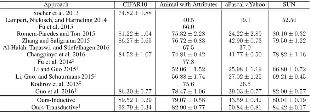
Table 2: The results on four benchmark datasets. The symbol‡indicates that the approach is in the transductive setting.
Approach CIFAR10 Animal with Attributes aPascal-aYahoo SUN
Socher et al. 2013 74.82±0.88
Lampert, Nickisch, and Harmeling 2014 40.5 19.1 52.50
Fu et al. 2015 66.0
Romera-Paredes and Torr 2015 81.22±1.04 75.32±2.28 24.22±2.89 80.10±0.32 Zhang and Saligrama 2015 86.27±0.65 76.72±0.83 42.90±0.73 79.50±1.22
Al-Halah, Tapaswi, and Stiefelhagen 2016 67.5 37.0
Changpinyo et al. 2016 84.52±1.07 74.81±0.42 41.77±0.50 78.82±1.16
Fu et al. 2014‡ 77.8
Li and Guo 2015‡ 52.06±1.52 25.98±1.19 66.80±0.72
Li, Guo, and Schuurmans 2015‡ 56.88±1.74 27.02±1.25 69.21±0.45
Kodirov et al. 2015‡ 75.6 26.5
Guo et al. 2016‡ 86.30±0.77 78.47±1.06 39.03±0.77 82.00±0.57
Ours-Inductive 89.52±0.29 79.07±0.58 43.59±0.42 80.04±0.19 Ours-Transductive‡ 92.79±0.34 82.90±0.77 50.84±0.81 84.42±0.17
Initialization and Iterative Refinement
In the transductive setting where the unlabeled target sam-ples are available, to solve Eq. (4), the estimated labels ˜
c(xj)should be given. However, there is no model to es-timate them at first. In this paper, we propose to use an itera-tive refinement procedure to address the initialization prob-lem. Specifically, at the first iteration, we ignore the sec-ond part in Eq. (4) and learn the projection only with the labeled source samples. Then we perform the sample selec-tion, pseudo label assignment, and robust SVM training se-quentially. Having obtained the classifiers for target classes, the estimated labels can be generated. Next, we can solve Eq. (4) based on the target samples and estimated labels and afterwards it can result in a better projection. With a better projection, the whole procedure is re-executed and we nor-mally expect to generate more effective classifiers for target classes which refine the estimated labels. Therefore, we pro-pose to iteratively refine the estimated labels and models un-til convergence. In the coming experiment, we will demon-strate that the iterative refinement can always lead to better results. On the other hand, in the inductive setting where no target sample is available. We just need to ignore the second part in Eq. (4) and run the procedure by only one iteration.
Experiment
Settings
We conduct experiments on four datasets. The first one is CIFAR10 (Krizhevsky 2009) which has10 object classes. There are 6,000images in each class. Following (Socher et al. 2013), in each split, we select 2 classes as the tar-get classes and the other8 as the source classes, and thus we have C2
10 = 45 different splits. The second database is Animal with Attributes (AwA) (Lampert, Nickisch, and Harmeling 2014) dataset which consists of50animal classes and30,475images. Following the split suggested in (Lam-pert, Nickisch, and Harmeling 2014),40classes with24,295 images are adopted as the source classes and 10 classes with 6,180images are adopted as the target classes. The third one is aPascal-aYahoo (aPY) dataset (Farhadi et al.
2009), in which aPascal has 20objects designed for PAS-CAL VOC2008 challenge, such as “people” and “dog”. It contains in total 12,695images. aYahoo dataset was col-lected from Yahoo image search. It has 12 classes which are similar but different from the ones in aPascal, such as “cen-taur” and “wolf”. It contains2,644images. We regard aPas-cal as the source classes and aYahoo as the target classes. The last one is SUN scene recognition dataset (Patterson and Hays 2012). It has717scenes and each scene has20images. We use707classes as the source and10as the target follow-ing the settfollow-ing from (Jayaraman and Grauman 2014). For CI-FAR10, the class attributes are the50-dimensional word rep-resentation learned by (Huang et al. 2012). For AwA, aPY, and SUN, we use the attributes provided by the dataset. For each image, we utilize the4096-dimensional features from fc7 layer of the pre-trained AlexNet (Krizhevsky, Sutskever, and Hinton 2012). Finally, the performance is evaluated by the multi-class classification accuracy on the target classes.
To implement our approach, we use the following setting. As introduced above, we select samples for each target class individually. In the inductive setting, for each target class, we selectms = 500,500,200,200source samples for CI-FAR10, AwA, aPY, and SUN respectively. In the transduc-tive setting, we further select mt = 500,200,50,10from unlabeled target samples. In addition, to determine the pa-rameter value forβ for sample selection,µandCfor train-ing robust SVM, we adopt the claswise crosvalidation s-trategy (Zhang and Saligrama 2015; Guo et al. 2016) where
β and C are chosen from {10−2,10−1,1,10,102} and µ is from {0,0.025,0.05, ...,0.2}. We report the results of both inductive and transductive versions of our approach and compare them to the baseline approaches from both settings.
Benchmark Comparison
0 0.05 0.1 0.15 0.2 50
60 70 80 90 100
µ
Accuracy (%) airplane−frog cat−dog bird−cat
(a) CIFAR10
0 0.05 0.1 0.15 0.2
60 70 80 90
µ
Accuracy (%)
(b) AwA
0 0.05 0.1 0.15 0.2
30 40 50 60
µ
Accuracy (%)
(c) aPY
0 0.05 0.1 0.15 0.2
60 70 80 90
µ
Accuracy (%)
[image:6.612.87.519.51.368.2](d) SUN
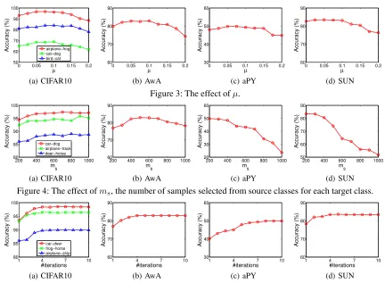
Figure 3: The effect ofµ.
200 400 600 800 1000
80 85 90 95 100
ms Accuracy (%) car−dogairplane−track
deer−horse
(a) CIFAR10
200 400 600 800 1000
60 70 80 90
ms
Accuracy (%)
(b) AwA
200 400 600 800 1000
20 30 40 50 60
ms
Accuracy (%)
(c) aPY
200 400 600 800 1000
50 60 70 80 90
ms
Accuracy (%)
(d) SUN
Figure 4: The effect ofms, the number of samples selected from source classes for each target class.
1 4 7 10
80 85 90 95 100
#iterations Accuracy (%) car−deer
frog−horse airplane−ship
(a) CIFAR10
1 4 7 10
60 70 80 90
#iterations
Accuracy (%)
(b) AwA
1 4 7 10
30 40 50 60
#iterations
Accuracy (%)
(c) aPY
1 4 7 10
60 70 80 90
#iterations
Accuracy (%)
(d) SUN
Figure 5: The classification accuracy w.r.t. the number of iterations.
better than the two-step strategy because it suffers from less information loss. Meanwhile, it also proves that our sample selection algorithm can choose samples from source classes that can well capture the characteristics of the target class.
More Results
Now we investigate some important issues of our approach. Because of the space limitation, we only discuss the trans-ductive version. In fact, the intrans-ductive one has similar trends. We first investigate how our approach behaves when vary-ing ofµin robust SVM. The results w.r.t. different values of
µ on four datasets are are shown in Figure 3. On the one hand, ifµis too small, the label noise will affect the quality of the classifiers. On the other hand, ifµis too large, the re-lationship between samples will be neglected such that the information may be not enough to train effective classifiers. Empirically, we can chooseµ∈[0.05,0.1]for our approach. The influence of the number of selected samples from source classes for each target class, i.e.,ms, is presented in Figure 4. For CIFAR10, the increase of performance is pro-portional to the rise in selected sample number. For AwA, more samples lead to better performance whenms < 600 but lead to worse performance when ms > 600. For the other two datasets, increasingmsmay result in worse per-formance. The reason is as follows. The main assumption for our approach is that there exists some samples in source classes that are verysimilarto target classes and thus we can use them to capture the characteristics of target classes, as illustrated in Figure 2. For CIFAR10, it has a large
candi-date set and thus there may exist a lot of good samples such that selecting more samples leads to better result. However, in aPY and SUN, the candidate set is small, so that there is only a few good samples (ms < 400). Whenms is large, many dissimilar (bad) samples are mistakenly selected such that they fail to effectively describe the target classes. We leave how to determinemsautomatically to our future work. In the transductive setting, we propose an iterative algo-rithm to progressively refine the estimated labels and the models. In Figure 5, we plot the accuracy on the test set w.r.t. the number of iterations. Obviously, the accuracy increases steadily at beginning and remains stable after10iterations, which validates the effectiveness of the iterative refinement.
Conclusion
References
Akata, Z.; Perronnin, F.; Harchaoui, Z.; and Schmid, C. 2013. Label-embedding for attribute-based classification. In2013 IEEE Conference on Computer Vision and Pattern Recognition, 819–826.
Al-Halah, Z.; Tapaswi, M.; and Stiefelhagen, R. 2016. Re-covering the missing link: Predicting class-attribute associa-tions for unsupervised zero-shot learning. InCVPR. Belkin, M., and Niyogi, P. 2001. Laplacian eigenmaps and spectral techniques for embedding and clustering. In Ad-vances in Neural Information Processing Systems 14, 585– 591.
Bertsekas, D. 1999.Nonlinear programming. Belmont,MA: Athena Scientific.
Bishop, C. M., et al. 2006.Pattern recognition and machine learning, volume 1. Springer, New York.
Chang, C., and Lin, C. 2011. LIBSVM: A library for support vector machines.ACM TIST2(3):27.
Changpinyo, S.; Chao, W.; Gong, B.; and Sha, F. 2016. Synthesized classifiers for zero-shot learning. In2016 IEEE Computer Society Conference on Computer Vision and Pat-tern Recognition.
Cortes, C., and Vapnik, V. 1995. Support-vector networks.
Machine Learning20(3):273–297.
Farhadi, A.; Endres, I.; Hoiem, D.; and Forsyth, D. A. 2009. Describing objects by their attributes. In2009 IEEE Com-puter Society Conference on ComCom-puter Vision and Pattern Recognition, 1778–1785.
Frome, A.; Corrado, G. S.; Shlens, J.; Bengio, S.; Dean, J.; Ranzato, M.; and Mikolov, T. 2013. Devise: A deep visual-semantic embedding model. In27th Annual Conference on Neural Information Processing Systems 2013, 2121–2129.
Fu, Y.; Hospedales, T. M.; Xiang, T.; Fu, Z.; and Gong, S. 2014. Transductive multi-view embedding for zero-shot recognition and annotation. In Computer Vision - ECCV 2014 - 13th European Conference, 584–599.
Fu, Z.; Xiang, T.; Kodirov, E.; and Gong, S. 2015. Zero-shot object recognition by semantic manifold distance. In2015 IEEE Computer Society Conference on Computer Vision and Pattern Recognition.
Guo, Y.; Ding, G.; Jin, X.; and Wang, J. 2016. Transductive zero-shot recognition via shared model space learning. In
Proceedings of the Thirtieth AAAI Conference on Artificial Intelligence.
Huang, E. H.; Socher, R.; Manning, C. D.; and Ng, A. Y. 2012. Improving word representations via global context and multiple word prototypes. InThe 50th Annual Meeting of the Association for Computational Linguistics, 873–882. Jayaraman, D., and Grauman, K. 2014. Zero-shot recog-nition with unreliable attributes. InAnnual Conference on Neural Information Processing Systems 2014, 3464–3472.
Kodirov, E.; Xiang, T.; Fu, Z.; and Gong, S. 2015. Unsu-pervised domain adaptation for zero-shot learning. InIEEE International Conference on Computer Vision.
Krizhevsky, A.; Sutskever, I.; and Hinton, G. E. 2012. Ima-genet classification with deep convolutional neural network-s. InAdvances in Neural Information Processing Systems 25, 1106–1114.
Krizhevsky, A. 2009. Learning multiple layers of features from tiny images.Tech Report. Univ. of Toronto.
Lampert, C. H.; Nickisch, H.; and Harmeling, S. 2009. Learning to detect unseen object classes by between-class attribute transfer. In2009 IEEE Computer Society Confer-ence on Computer Vision and Pattern Recognition, 951–958. Lampert, C. H.; Nickisch, H.; and Harmeling, S. 2014. Attribute-based classification for zero-shot visual objec-t caobjec-tegorizaobjec-tion. IEEE Trans. Pattern Anal. Mach. Intell.
36(3):453–465.
Li, X., and Guo, Y. 2015. Max-margin zero-shot learning for multi-class classification. InProceedings of the Eighteenth International Conference on Artificial Intelligence and S-tatistics.
Li, X.; Guo, Y.; and Schuurmans, D. 2015. Semi-supervised zero-shot classification with label representation learning. In
IEEE International Conference on Computer Vision. Norouzi, M.; Mikolov, T.; Bengio, S.; Singer, Y.; Shlens, J.; Frome, A.; Corrado, G.; and Dean, J. 2013. Zero-shot learn-ing by convex combination of semantic embeddlearn-ings. CoRR
abs/1312.5650.
Patterson, G., and Hays, J. 2012. SUN attribute database: Discovering, annotating, and recognizing scene attributes. In2012 IEEE Conference on Computer Vision and Pattern Recognition, 2751–2758.
Romera-Paredes, B., and Torr, P. H. S. 2015. An embarrass-ingly simple approach to zero-shot learning. InProceedings of the 32nd International Conference on Machine Learning, 2152–2161.
Socher, R.; Ganjoo, M.; Manning, C. D.; and Ng, A. Y. 2013. Zero-shot learning through cross-modal transfer. In27th An-nual Conference on Neural Information Processing Systems 2013, 935–943.
Spielman, D. A., and Teng, S. 2004. Nearly-linear time algorithms for graph partitioning, graph sparsification, and solving linear systems. InProceedings of the 36th Annual ACM Symposium on Theory of Computing, 81–90.