Direct numerical simulation of a turbulent 90º bend pipe flow

Manuscript version: Author’s Accepted Manuscript

The version presented in WRAP is the author’s accepted manuscript and may differ from the published version or Version of Record.

Persistent WRAP URL:

http://wrap.warwick.ac.uk/106812

How to cite:

Please refer to published version for the most recent bibliographic citation information. If a published version is known of, the repository item page linked to above, will contain details on accessing it.

Copyright and reuse:

The Warwick Research Archive Portal (WRAP) makes this work by researchers of the University of Warwick available open access under the following conditions.

© 2019 Elsevier. Licensed under the Creative Commons Attribution-NonCommercial-NoDerivatives 4.0 International http://creativecommons.org/licenses/by-nc-nd/4.0/.

Publisher’s statement:

Please refer to the repository item page, publisher’s statement section, for further information.

Direct numerical simulation of a turbulent

90

◦

bend pipe flow

Zhixin Wang

, Ramis ¨

Orl¨

u

, Philipp Schlatter

and Yongmann M. Chung

1

_{School of Engineering, University of Warwick, Coventry CV4 7AL, UK}

2

_Linn´

_{e FLOW Centre, KTH Mechanics SE-100 44, Stockholm, Sweden}

Abstract

Direct numerical simulation (DNS) has been performed for a spatially

develop-ing 90◦ bend pipe flow to investigate the unsteady flow motions downstream of the bend. A recycling method is implemented to generate a fully-developed turbulent

inflow condition. The Reynolds number of the pipe flow is ReD = 5300 and the

bend curvature is γ = 0.4. A long straight pipe section (40D) is attached in the

downstream of the bend to allow the flow to develop. Flow oscillations downstream

of the bend are measured using several methods, and the corresponding oscillation

frequencies are estimated. It is found that different characteristic frequencies are

obtained from various flow measurements. The stagnation point movement and

single-point velocity measurements may not be good measures to determine the

swirl-switching frequency. The oscillations of the lateral pressure force on the pipe

wall and half-sided mass flow rate are proposed to be a more unambiguous measure

of the unsteady flow motions downstream of the bend.

1

Introduction

Turbulent flow in 90◦ pipe bends is encountered in many engineering applications, and attracted a significant interest in recent years. Many experimental studies focused on

flow oscillations related to thermal and mechanical fatigue in industrial pipeline systems,

and some numerical studies tackle more fundamental issues regarding the secondary flow

oscillations in bend pipes. An extensive literature review is available in Kalpakli Vester

Apart from the practical aspects, one of the most intriguing fundamental problems

arises from turbulent pipe flow with 90◦bends is the so-calledswirl-switchingphenomenon (Tunstall and Harvey, 1968; Br¨ucker, 1998). This phenomenon is associated with the

unsteady motions of the Dean vortices (Dean, 1927, 1928) downstream of 90◦ bends. It has been the focus of many studies in the past two decades (R¨utten et al., 2001, 2005;

Ebara et al., 2010; Ono et al., 2011; Takamura et al., 2012; Sakakibara and Machida,

2012; Kalpakli et al., 2012; Kalpakli and ¨Orl¨u, 2013; Kalpakli et al., 2013; Hellstr¨om

et al., 2013; Kalpakli Vester et al., 2015; Carlsson et al., 2015; Tunstall et al., 2016;

Noorani and Schlatter, 2016; Wang and Chung, 2017; Chung and Wang, 2017), and this

phenomenon is directly associated with the thermal and mechanical fatigue in pipeline

systems.

It is interesting to see that various flow properties have been used to study the

swirl-switching phenomenon in previous studies; of particular interest has been the

determina-tion of the swirl-switching frequency. Br¨ucker (1998) used filtered streamwise vorticity

from his PIV experiments, and the filtering was applied to reduce the noise from the PIV

data. Velocity fluctuations on the symmetry plane were used by Takamura et al. (2012);

Sakakibara and Machida (2012), while pressure fluctuations were used by Ebara et al.

(2010); they all reported a frequency of St= 0.5. The variation of the outer stagnation

point of the Dean vortices was used by R¨utten et al. (2001, 2005). 2D POD (proper

or-thogonal decomposition) was employed in several experimental (Kalpakli and ¨Orl¨u, 2013;

Hellstr¨om et al., 2013; Kalpakli Vester et al., 2015) and numerical (Carlsson et al., 2015;

Tunstall et al., 2016) studies, but the results are found to be inconclusive. This clearly

shows the difficulty in measuring the swirl-switching frequency. Recently, Hufnagel et al.

(2018) found that 2D POD is not appropriate for the analysis of the swirl-switching

frequency, and they argued that instead 3D POD should be used. However, 3D POD

would be out of reach for most experimental studies. In this paper, we first review several

methods used in literature to study the swirl-switching phenomenon, and propose two

simple measures of the swirl-switching frequency.

As pointed out in a review paper by Kalpakli Vester et al. (2016), the three-dimensional

phenomenon. Most of previous numerical studies on 90◦ bend pipe flow were performed using large-eddy simulation (LES) (Boersma and Nieuwstadt, 1996; R¨utten et al., 2001,

2005; Carlsson et al., 2015; R¨ohrig et al., 2015; Tunstall et al., 2016). DNS studies have

only started recently (Wang and Chung, 2016, 2017; Chung and Wang, 2017; Hufnagel

et al., 2018). In the present study, DNS of a spatially developing turbulent pipe flow with

a 90◦ bend has been performed at γ = 0.4 and ReD = 5300. The main aim is to assess different flow measurement methods associated with the swirl-switching phenomenon.

2

Computational details

2.1

Governing equations

The high-order spectral element method code, Nek5000 (Fischer et al., 2008), is used to

perform DNS of a spatially developing 90◦ bend pipe flow. The flow is governed by the incompressible Navier-Stokes equations,

∂ui ∂xi

= 0, (1)

∂ui ∂t +uj

∂ui ∂xj

= −∂p

∂xi

+ 1

ReD ∂2ui ∂xj∂xj

. (2)

Nek5000 is written in FORTRAN and C, and parallelised using MPI technique. The

governing equations are solved in Cartesian coordinates. The computational domain is

comprised of local hexahedral elements, and each element is further refined by structured

Gauss-Lobatto-Legendre (GLL) nodes. The velocity solution space is represented by a

basis ofN-th order Lagrange polynomials on the GLL points, while the pressure solution

space on the Gauss-Legendre points is two orders lower than the velocity. This is known

as the _PN −PN−2 method detailed in Maday and Patera (1989). The polynomial order was set to be N = 7 in the present DNS study. A third-order semi-implicit method was

used for the time advancement.

In the present paper, the Reynolds number is defined as ReD = UmD/ν, where Um is the bulk mean velocity in the pipe, D is the pipe diameter, and ν is the kinematic

ReD γ Lrecyc Lout Grid points ∆z+, ∆r+, R∆θ+ N

5300 0.4 25R 80R 105×106 _{[3.03, 9.91], [0.14, 4.36], [1.51, 4.93] 7}

Table 1: Simulation parameters of the turbulent 90◦ bend pipe flow DNS.

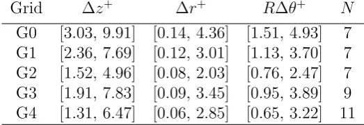
Grid ∆z+ _∆r+ _R∆θ+ _N

G0 [3.03, 9.91] [0.14, 4.36] [1.51, 4.93] 7

G1 [2.36, 7.69] [0.12, 3.01] [1.13, 3.70] 7

G2 [1.52, 4.96] [0.08, 2.03] [0.76, 2.47] 7

G3 [1.91, 7.83] [0.09, 3.45] [0.95, 3.89] 9

G4 [1.31, 6.47] [0.06, 2.85] [0.65, 3.22] 11

Table 2: Grid resolutions used in the grid independence study.

radius R(≡ D/2) to the mean curvature radius at the pipe centreline Rc. Details of the simulation parameters are summarised in Table 1. The total length of the pipe is more

than 120R, including the bend.

2.2

Grid sensitivity study

A grid independence study was performed to determine the necessary grid resolutions

for the simulation. A cylindrical grid was chosen for the near-wall region between 0.8≤

r/R ≤ 1, so that no extra interpolation was needed for the data processing within this

near-wall region to calculate near-wall turbulence statistics. The sizes of elements were

set to increase gradually within the cylindrical region whilst uniform outside this region

towards the pipe centre. Five different grids (details are shown in Table 2) were used

for DNSs at ReD = 5300 with a pipe length of L/R = 10. Please note that the grid

resolutions of G0 were similar to those in El Khoury et al. (2013). Both the element size

and the polynomial order were changed. G1 and G2 used more elements with the same

polynomial order of N = 7. G3 and G4 used higher polynomial orders while using the

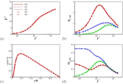
same number of elements as in G0. Several flow quantities including mean velocity, rms

of the velocity fluctuations, Reynolds shear stress and rms of the vorticity fluctuations are

shown in figure 1. The DNS results show no discernible difference between the five grids

considered. Therefore, the baseline grid resolution (G0) was used for the main turbulent

pipe flow simulations. In grid G0, ∆r+

(a) y+ U + 100 101 102 0 5 10 15 20 25 G0 G1 G2 G3 G4

(b) y+

ui, rm s 100 101 102 0 1 2 3 (c) y/R -< u ’v ’>

0 0.2 0.4 0.6 0.8 1

0 0.2 0.4 0.6 0.8 1

(d) y+

ω

i,

rm

s

100 101 102 0

0.1 0.2 0.3 0.4

Figure 1: Comparison of (a) mean velocity, (b) rms of the velocity fluctuations, (c) Reynolds shear stress, and (d) rms of the vorticity fluctuations with five grid resolutions used. All variables are in wall units. Solid lines represent the results of G0 grid resolution, dashed and dash-dotted lines represent the results of G1 and G2 grid resolutions, and circles and triangles represent the results of G3 and G4 grid resolutions, respectively.

fourteen grid points below ∆r+ _{= 10, and ∆z}+

max ≤ 10 and R∆θmax+ ≤ 5, respectively. Note that similar grid strategy was used in the recent DNS study of a 90◦ bend pipe flow by Hufnagel et al. (2018).

2.3

Boundary condition

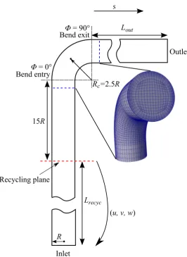
Figure 2 shows a schematic of the computational domain. In the present study, an

additional coordinate is introduced to analyse the downstream flow development after

the bend: s is defined as the distance in the downstream direction from the bend exit.

The origin of the coordinate is located at the bend exit (s/D = 0) as shown in figure 2.

The no-slip condition was applied at the pipe wall and the zero-stress outflow condition

R

L_recyc Recycling plane

Inlet

Outlet L_out

Rc=2.5R

15R

(u, v, w) Bend exitΦ = 90°

Bend entryΦ = 0°

s

Figure 2: Schematic of the computational domain.

a fully-developed turbulent inflow condition. The velocity solution of the present time

step un(Lrecyc, r, θ) is used as the Dirichlet condition at the pipe inlet for the next time step un+1_{(0, r, θ). This procedure is explicit in time and is carried out at every time} step during the simulation. Neither scaling nor interpolation is required when copying

the velocity to the inlet since the mesh is identical at all pipe cross-sections. In order to

obtain a fully-developed turbulent inflow condition, the recycling plane was chosen to be

Lrecyc/R = 25 according to the DNS study of pipe length effect on turbulence statistics (Chin et al., 2010). The recycling technique has been used in many numerical studies

(Chung and Sung, 1997). Figure 3 shows mean velocity and velocity fluctuations in the

upstream recycling section. The turbulence statistics show an excellent agreement with

the DNS data for the straight pipe flow (El Khoury et al., 2013; Chin et al., 2014) at the

(a) y+

U

+

100

101

102 0

5 10 15 20 25

El Khouryet al.(2013) Chinet al.(2014) Inflow

(b) y+

ui,

rm

s

100

101

102 0

1 2 3

El Khouryet al.(2013) Inflow

Figure 3: Comparison of (a) mean velocity and (b) rms of the velocity fluctuations at

ReD = 5300 (or Reτ = 180). All variables are in wall units. Solid lines represent the present bend pipe DNS. Symbols represent the DNS data of El Khoury et al. (2013) and Chin et al. (2014).

Figure 4: Time-averaged in-plane velocity magnitude (pu2

r+u2θ) and velocity vectors

at 1D downstream of the pipe bend (s/D = 1). I and O indicate the inner and outer

(a)

(b)

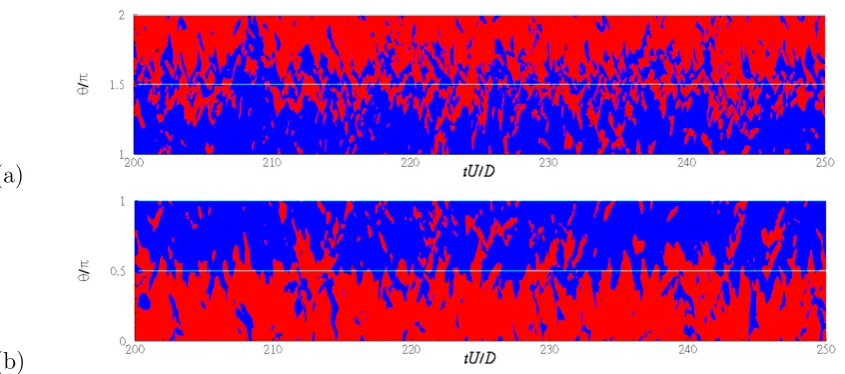
Figure 5: Time history of azimuthal velocity at first grid point from the pipe wall along (a) 1≤θ/π ≤2 and (b) 0≤θ/π ≤1. Red colour represents clockwise velocity and blue colour represents anticlockwise velocity.

3

Results and discussion

Figure 4 shows the time-averaged secondary flow motions at 1D downstream of the pipe

bend. A pair of counter-rotating vortices, i.e., the Dean vortices, are clearly seen, and

they are symmetric about the axis of symmetry (from the inner side “I” to the outer

side “O”). These vortex cells take turns to dominate in the instantaneous flow field.

To investigate the unsteady flow motions in the downstream of a 90◦ bend, several flow properties are measured from the present DNS dataset.

3.1

Stagnation point

In the time-averaged flow field (figure 4), the stagnation points of the in-plane flow

motions are easy to identify. Due to the oscillation of the Dean vortices, the stagnation

points also vary in time during the swirl-switching as shown in Br¨ucker (1998). Figures 5

and 6 show the time variations of azimuthal velocity at the first grid point and 0.05Rfrom

the pipe wall, respectively. The boundary between the clockwise (red) and anticlockwise

(blue) motions indicates the azimuthal positions of the stagnation point. The actual

position of the stagnation point is not clear. R¨utten et al. (2005) measured the position

(a)

(b)

Figure 6: Time history of azimuthal velocity at 0.05R from the pipe wall along (a) 1≤θ/π ≤2 and (b) 0≤θ/π ≤1. Colours are the same as in figure 5.

(a)

(b)

Figure 7: Time history of azimuthal velocity at 0.05R from the pipe wall along (a)

1 ≤ θ/π ≤ 2 and (b) 0 ≤ θ/π ≤ 1. Moving average is applied to the original data.

out that it is impossible to obtain an unambiguous signal of the stagnation point from

the original flow fields. A moving average with a window size of ∆t = 0.5 is applied

to the original data. Figure 7 shows the filtered velocity signal at 0.05R from the wall.

The oscillation of stagnation point becomes slightly more discernible, it is however still

difficult to extract the accurate positions. Sakakibara and Machida (2012) also measured

the stagnation point at 0.12R from the pipe wall using PIV data. They observed that

the oscillations of the inner stagnation point are quasi-periodic while the oscillations of

the outer stagnation point are more random.

In the present DNS, it is clearly seen that stagnation point movement is rather

com-plicated. It is also observed that these variations depend on the location of measurement.

As the location moves away from the pipe wall, the position of the stagnation point also

changes. There seems to be no dominant frequency from the variations of the stagnation

point, since the oscillation is slow during certain time periods while it becomes more

intensive at other times. In addition, it is probably hard to determine whether these

stagnation points are indeed representative of the swirl-switching phenomenon.

3.2

Velocity fluctuations

Time signals of velocity fluctuations at different locations downstream of the pipe bend

were also used in several studies (Br¨ucker, 1998; Takamura et al., 2012; Kalpakli and

¨

Orl¨u, 2013) to extract the characteristic frequency of the unsteady flow motions.

Typi-cally, azimuthal velocity near the axis of symmetry was measured close to the inner side

(Br¨ucker, 1998; Kalpakli and ¨Orl¨u, 2013). Multiple frequencies were reported from the

single-point velocity signals.

Figures 8 - 10 show the time variations and PSD (power spectral density) estimate

of streamwise, vertical and horizontal velocity fluctuations along the axis of symmetry at

s/D= 1, respectively. It is interesting to observe that for different velocity components,

strong fluctuations appear at different y/R locations. For the streamwise velocity

com-ponent, it is clear to see fluctuations with large amplitude within 0 < y/R <0.5 (figure

8(a)). Multiple oscillation frequencies are observed in this region (figure 8(c)). This strong

(a)

tU/D

us

130 135 140 145 150

-0.8 -0.6 -0.4 -0.2 0 0.2 0.4 0.6 0.8

(b) (c)

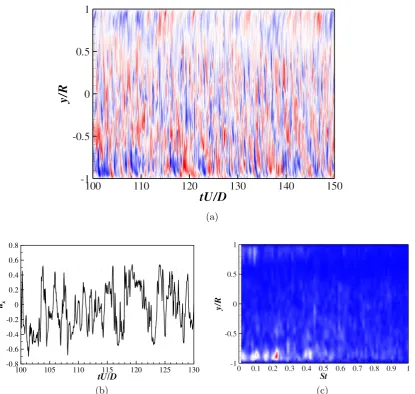
Figure 8: (a) 2D contour of streamwise velocity fluctuations along the axis of symmetry at

(a)

tU/D

uy

130 135 140 145 150 155 160

-0.8 -0.6 -0.4 -0.2 0 0.2 0.4 0.6 0.8

(b) (c)

(a)

tU/D

ux

100 105 110 115 120 125 130 -0.8

-0.6 -0.4 -0.2 0 0.2 0.4 0.6 0.8

(b) (c)

y/R

-1 -0.5 0 0.5 1

0 0.5 1 1.5

U

|dU/dy|/2

Figure 11: Time-averaged streamwise velocity U (solid line) and magnitude of velocity gradient |dU/dy| (dashed line) along the axis of symmetry at s/D = 1. The values of |dU/dy| are scaled by half.

shown clearly in figure 11. Similarly, the strong oscillation around y/R = −0.5 for

vertical velocity fluctuations (figures 9(a) and (c)) is associated with the shear layer at

−0.7 < y/R < −0.4 (figure 11). The dominant frequency within this region is around

St = 0.2−0.3, and this frequency could be attributed to the shear layer instability as

mentioned in R¨utten et al. (2005). For horizontal velocity fluctuations, stronger

oscilla-tion is located at −1< y/R <−0.5. This is due to the alternative motions of the Dean

vortices around the symmetry plane.

For all three velocity components, the time variations (figures 8(b), 9(b) and 10(b))

consist of fluctuations with different time scales (frequencies). It is also noticed that

velocity fluctuations near the outer side (0.5 < y/R < 1) are weak compared with

the other regions. Takamura et al. (2012) also showed that no characteristic velocity

fluctuations are observed close to the outer side downstream of the 90◦ bend. It is clearly seen that different characteristic frequencies can be extracted depending on the location of

measurement. The flow is dominated by different oscillatory motions in different regions.

Single-point measurement may not be able to distinguish the swirl-switching from the

tU/D

F

0 50 100 150 200 250 300

entry

s/D

upstream

s/D

s/D

s/D

s/D= 10

= 5

= 2

= 1

= 0

Figure 12: Horizontal component of wall pressure force at different pipe cross-sections: green, upstream recycling region; cyan, entry of the bend; purple, s/D = 0 (exit of the

bend); red, s/D = 1; blue, s/D = 2; orange, s/D = 5; and black, s/D = 10. The lines

are shifted away from each other to show the difference clearly.

3.3

Pressure force oscillation

Earlier studies (R¨utten et al., 2001, 2005) measured the total pressure force on the entire

pipe wall from upstream to downstream of the bend. In order to investigate the flow

oscillation in the downstream of the bend, the pressure force exerted on the pipe wall is

calculated along the streamwise direction.

G(s) = R

Z 2π

0

p(s, θ)ndθ,

where n is the normal vector to the pipe wall. In this study, the horizontal component

of pressure force on the pipe wall is monitored: F =G·ex, where ex is the unit vector

in the horizontal (x) direction (indicated in figure 4). The pressure force is chosen in this

study to capture the swirl-switching for two reasons: one is that the pressure force is a

global property, unlike local velocity or pressure used in previous studies; and the other

is that force oscillation is the property most relevant to the safety of the pipe system

design.

force fluctuation is highlighted. There are small force fluctuations in the straight pipe

section upstream the bend. It is clear to see that these small oscillations are enhanced

by the bend. At the bend exit (s/D= 0), force oscillations are already much larger than

the straight pipe value. They become even stronger after the bend, before they decrease

far downstream (s/D= 5). It is observed that the force oscillation reaches its maximum

value at s/D= 1.

It is worthwhile to note that the POD analysis has been used in several studies to

measure the swirl-switching frequency. The POD analysis can be viewed as a global

measure of the frequency. Although there is some discrepancy among POD studies,

Hufnagel et al. (2018) show a lower frequency from their 3D POD analysis whereas some

experiments (Takamura et al., 2012; Hellstr¨om et al., 2013) show St ≈ 0.5. Hufnagel

et al. (2018) suggest 3D POD can be used to extract the completely global coherent

modes including the streamwise dependence, while the streamwise dependency of the

frequency affects the 2D POD modes.

3.4

Mass flow rate oscillation

It has been observed from the instantaneous flow fields that, the streamwise velocity on

the left and right sides of the pipe oscillate during the swirl-switching. The unsteady

motions of the Dean vortices lead to mass flow rate imbalance between the left and right

sides. To investigate the streamwise flow oscillation, mass flow rates on the left (qL) and right (qR) sides of the pipe are monitored.

Figure 13 shows the time history of normalised mass flow fluctuation on the left

side of the pipe (q_L0 ) together with the horizontal force fluctuation F. Both force and mass flow rate fluctuations are quasi-periodic, and a strong correlation between these two

fluctuations can be observed. The horizontal force fluctuation appears to be associated

with two frequencies: St≈0.5 and 1.0. This is clearly seen in figure 13. The blue region

(around t= 140) indicates where St≈0.5 is dominant and the green region (aroundt=

160) indicates St≈ 1.0. The flow rate fluctuation is clearly associated with a frequency

of St = 0.5. Spectral analysis shows that St ≈ 0.5 is the most dominant frequency for

tU/D

130 140 150 160 170

-5 -4 -3 -2 -1 0 1 2 3 4 5

Horizontal force Mass flow rate

Figure 13: Time history of mass flow fluctuation,q_L0 /σq (thick black line) on the left side of the pipe and horizontal force fluctuation, F/σF (thin grey line) at s/D= 1. Both q0L and F are normalised by the corresponding standard deviations. Fluctuations in solid blue circle depict St≈0.5. Fluctuations in dashed green circle depict St≈1.0.

bend pipe experimental (St≈ 0.5) (Ebara et al., 2010; Takamura et al., 2012) and LES

(St = 0.5−0.6) (Carlsson et al., 2015) studies. The frequency of St ≈ 0.5 appears to

be Reynolds number independent in the experiments using pressure fluctuations (Ebara

et al., 2010) and circumferential velocity fluctuations (Takamura et al., 2012). Carlsson

et al. (2015) suggested that this switching frequency in their LES study was an intrinsic

feature of the bend as it became more dominant when the bend was sharper. It is also

noted that relatively sharp bends (γ ≥ 0.32) were used in their studies, similar to the

present study (γ = 0.4).

Figure 14 shows the autocorrelations of the mass flow rate fluctuations on the left

side of the pipe downstream of the bend. The effect of the bend is clearly seen as strong

flow rate oscillation is observed up to s/D ≈ 8, before it decays further downstream.

The oscillation frequency read from the autocorrelations is St ≈0.5, and this frequency

remains largely unchanged up to s/D ≈ 6. The measurements of horizontal force and

mass flow rate oscillations are not dependent on the location of the in-plane flow motions.

0

5

100 5

10 15

20

0 0.5 1

C

s/D

∆

t

Figure 14: Autocorrelations of the flow rate fluctuation on the left side of the pipe

Cqq(∆t) = hq(t)q(t+ ∆t)i/σq2 in the downstream of the pipe bend.

swirl-switching is clear to observe (up tos/D≈6 in the present simulation). Hence, these

integrated values are more suitable for measuring the unsteady flow motions downstream

of the bend in comparison to single-point measurements.

3.5

Comparison of various methods

To summarise and conclude the four different ways of extracting information about the

swirl-switching phenomenon, this section presents the power spectra of the time-signals

from these methods. The power spectra of the time signals from velocity fluctuations

(section 3.2) are already presented in figures 8c), 9c) and 10c) and can therefore directly

be extracted for a certainy/R location, here chosen to be the one shown in figure 8b), i.e.

y/R = 0.1. The in-plane stagnation point is the location expressed as the demarcation

between clockwise and anticlockwise azimuthal velocity and can hence easily be extracted.

This demarcation appears as two azimuthal locations as apparent from figure 7, and the

PSD is based on the time-signal extracted through a boundary/edge detection algorithm:

Since figure 7 was obtained upon application of a moving average, the same short-time

average was also applied on the other time-series signals discussed in this section. The

comparably lowSt values from 0.05 to 0.3. The global measures instead, i.e. the PSD of

the time series for the horizontal forceF and mass-flow on the left side of the pipe, yield

dominant frequencies that are more comparable with the values that could visually be

observed in figure 13, i.e. St≈ 0.5. In agreement with the literature it is apparent that

methods based on the stagnation point as well as velocity fluctuations are rather

ambigu-ous and thus unsuited to obtain the swirl-switching frequency. Nonetheless, it should be

noted that, employing spatially-low-pass-filtered velocity fields, these methods seem to

provide better and more robust estimates (R¨utten et al., 2005; Sakakibara and Machida,

2012), although the method based on the velocity fluctuations is strongly dependent on

the selected location (cf. subplots c) in figures 8–10). These disadvantages seem to be

circumvented when using global measures such as the pressure force on the pipe or

mass-flow fluctuations. It is also reassuring to see that the latter two find the same dominant

frequency. Similarly, more involved and complicated global measures such as e.g. 3D

POD as performed in Hufnagel et al. (2018) seem to give equally robust measures, but

are not always practical.

4

Conclusions

In this study, the swirl-switching phenomenon in a 90◦ curved pipe is investigated by direct numerical simulations. A recycling turbulent inflow boundary condition was

im-plemented to simulate a spatially developing turbulent bend pipe flow. The Reynolds

number considered is ReD = 5300 and the bend curvature is γ = 0.4. The DNS bend

pipe data were analysed to study the unsteady oscillations of the Dean vortices. The

stagnation points, velocity fluctuations, horizontal component of the pressure force on

the pipe wall, and half-sided mass flow rate were monitored to study unsteady flow

mo-tions associated with the swirl-switching. It is shown that the stagnation points are

difficult to extract, and the actual position depends on the location of measurement.

Time series and PSD analysis of velocity fluctuations along axis of symmetry clearly

show that multiple dominant frequencies exist in the flow, and these frequencies vary in

different flow regions. Single point analysis may be biased due to the chosen location of

con-0 2 4 PSD(u =0) 0 1 2 PSD(u s ) 0 0.5 1 1.5 PSD(F)

0 0.1 0.2 0.3 0.4 0.5 0.6 0.7 0.8 0.9 1

St 0 1 2 3 PSD(q L )

Figure 15: PSD estimate of the time-signals for a) the (in-plane) stagnation point (dashed and solid line corresponding to the demarcation in figure 7a) and b), respectively), b) the streamwise velocity signal at y/R = 0.1 (in figure 8b), c) the horizontal force F, and d) the mass-flow on the left side of the pipe qL (both shown in figure 13). All time-signals are fluctuating parts that are normalised with their respective standard deviation.

sidered when measuring the velocity fluctuations. A measurement of lateral wall pressure

force is proposed, and it is found that the bend amplifies the force oscillations. The force

oscillation has a maximum value at 1D downstream of the bend. It is also observed that

the oscillation of the mass flow rate is strongly correlated with the horizontal force

oscilla-tion. The most dominant frequency for both force and mean flow oscillations is St≈0.5.

This frequency was also observed in several previous experiments. The quasi-periodic

behaviour of these two oscillations persist for a distance of s/D ≈ 6 before they decay

further downstream. Integrated flow quantities show more consistency compared to

mea-sures deduced from single-point measurements, and should be considered more suitable

for measuring the swirl-switching phenomenon. The present study shows that, despite a

large body of previous work, the flow in bend pipes turns out to be complicated. Not

only is the origin of the swirl-switching is unclear, even its characterisation appears to

depend on the specific measure, the geometry and flow rate. This contribution shows the

explains some of the disparity of data in the literature.

Acknowledgement

This work has been supported by the Engineering and Physical Sciences Research Council

grant no EP/L000261/1. The authors would like to thank Professor Paul Fischer for the

help in using Nek5000. Simulations were performed on ARCHER, the UK National

Supercomputing Service. This work also used the HPC facilities (Tinis) at the Centre

for Scientific Computing, University of Warwick.

References

B. J. Boersma and F. T. M. Nieuwstadt. Large-eddy simulation of turbulent flow in a

curved pipe. ASME: Journal of Fluids Engineering, 118(2):248–254, 1996.

Ch. Br¨ucker. A time-recording DPIV-study of the swirl switching effect in a 90◦ bend flow. In 8th International Symposium on Flow Visualisation, pages 171.1–171.6, 1-4

September, Sorrento, Italy, 1998.

C. Carlsson, E. Alenius, and L. Fuchs. Swirl switching in turbulent flow through 90◦ pipe bends. Physics of Fluids, 27:085112, 2015.

C. Chin, A. S. H. Ooi, I. Marusic, and H. M. Blackburn. The influence of pipe length

on turbulence statistics computed from direct numerical simulation data. Physics of

Fluids, 22(11):115107, 2010.

C. Chin, J. P. Monty, and A. Ooi. Reynolds number effects in DNS of pipe flow and

comparison with channels and boundary layers. International Journal of Heat and

Fluid Flow, 45:33–40, 2014.

Y. M. Chung and H. J. Sung. Comparative study of inflow conditions for

Y. M. Chung and Z. Wang. Direct numerical simulation of a turbulent curved pipe flow

with a 90◦ bend. In Turbulence and Shear Flow Phenomena -10, 6-9 July, Chicago, USA, 2017.

W. R. Dean. Note on the motion of fluid in a curved pipe. Philosophical Magazine, 4

(20):208–223, 1927.

W. R. Dean. The stream-line motion of fluid in a curved pipe. Philosophical Magazine,

5(30):673–695, 1928.

S. Ebara, Y. Aoya, T. Sato, H. Hashizume, Y. Kazuhisa, K. Aizawa, and H. Yamano.

Pressure fluctuation characteristics of complex turbulent flow in a single elbow with

small curvature radius for a Sodium-cooled fast reactor. ASME: Journal of Fluids

Engineering, 132(11):111102, 2010.

G. K. El Khoury, P. Schlatter, A. Noorani, P. F. Fischer, G. Brethouwer, and A. V.

Johansson. Direct numerical simulation of turbulent pipe flow at moderately high

Reynolds numbers. Flow, Turbulence and Combustion, 91(3):475–495, 2013.

P. F. Fischer, J. W. Lottes, and S. G. Kerkemeier. nek5000 Web page, 2008.

http://nek5000.mcs.anl.gov.

L. H. O. Hellstr¨om, M. B. Zlatinov, G. Cao, and A. J. Smits. Turbulent pipe flow

downstream of a 90◦ bend. Journal of Fluid Mechanics, 735:R7, 2013.

L. Hufnagel, J. Canton, R. ¨Orl¨u, O. Marin, E. Merzari, and P. Schlatter. The

three-dimensional structure of swirl-switching in bent pipe flow. Journal of Fluid Mechanics,

835:86–101, 2018.

A. Kalpakli and R. ¨Orl¨u. Turbulent pipe flow downstream a 90◦ pipe bend with and without superimposed swirl. International Journal of Heat and Fluid Flow, 41:103–

111, 2013.

A. Kalpakli, R. ¨Orl¨u, and P. H. Alfredsson. Dean vortices in turbulent flows: rocking or

A. Kalpakli, R. ¨Orl¨u, and P. H. Alfredsson. Vortical patterns in turbulent flow

down-stream a 90◦ curved pipe at high Womersley numbers. International Journal of Heat

and Fluid Flow, 44:692–699, 2013.

A. Kalpakli Vester, R. ¨Orl¨u, and P. H. Alfredsson. POD analysis of the turbulent flow

downstream a mild and sharp bend. Experiments in Fluids, 56(3):57, 2015.

A. Kalpakli Vester, R. ¨Orl¨u, and P. H. Alfredsson. Turbulent flows in curved pipes:

recent advances in experiments and simulations. Applied Mechanics Review, 68(5):

050802, 2016.

Y. Maday and A. T. Patera. Spectral element methods for the Navier-Stokes equations.

State of the Art Surveys in Computational Mechanics ASME, pages 71–143, 1989.

A. Noorani and P. Schlatter. Swirl-switching phenomenon in turbulent flow through

toroidal pipes. International Journal of Heat and Fluid Flow, 61:108–116, 2016.

A. Ono, N. Kimura, H. Kamide, and A. Tobita. Influence of elbow curvature on flow

structure at elbow outlet under high Reynolds number condition. Nuclear Engineering

and Design, 241(11):4409–4419, 2011.

R. R¨ohrig, S. Jakirli´c, and C. Tropea. Comparative computational study of turbulent

flow in a 90◦ pipe elbow. International Journal of Heat and Fluid Flow, 55:120–131, 2015.

F. R¨utten, M. Meinke, and W. Schr¨oder. Large-eddy simulations of 90◦ pipe bend flows.

Journal of Turbulence, 2(3):1–14, 2001.

F. R¨utten, W. Schr¨oder, and M. Meinke. Large-eddy simulations of low frequency

os-cillations of the Dean vortices in turbulent pipe bend flows. Physics of Fluids, 17(3):

035107, 2005.

J. Sakakibara and N. Machida. Measurement of turbulent flow upstream and downstream

of a circular pipe bend. Physics of Fluids, 24(4):041702, 2012.

short elbow piping under high Reynolds number condition. ASME: Journal of Fluids

Engineering, 134(10):101201, 2012.

M. J. Tunstall and J. K. Harvey. On the effect of a sharp bend in a fully developed

turbulent pipe-flow. Journal of Fluid Mechanics, 34:595–608, 1968.

R. Tunstall, D. Laurence, R. Prosser, and A. Skillen. Large eddy simulation of a

T-junction with upstream elbow: The role of Dean vortices in thermal fatigue. Appled

Thermal Engineering, 107:672–680, 2016.

Z. Wang and Y. M. Chung. Direct numerical simulation of a turbulent curved pipe flow.

In 11th European Fluid Mechanics Conference, 12-16 September, Seville, Spain, 2016.

Z. Wang and Y. M. Chung. DNS of turbulent pipe flow with a 90 degrees bend. In