Shadows don’t lie : n sequence trajectory inspection for misbehaviour detection and classification in VANETs

warwick.ac.uk/lib-publications

Manuscript version: Author’s Accepted Manuscript

The version presented in WRAP is the author’s accepted manuscript and may differ from the

published version or Version of Record.

Persistent WRAP URL:

http://wrap.warwick.ac.uk/127560

How to cite:

Please refer to published version for the most recent bibliographic citation information.

If a published version is known of, the repository item page linked to above, will contain

details on accessing it.

Copyright and reuse:

The Warwick Research Archive Portal (WRAP) makes this work by researchers of the

University of Warwick available open access under the following conditions.

Copyright © and all moral rights to the version of the paper presented here belong to the

individual author(s) and/or other copyright owners. To the extent reasonable and

practicable the material made available in WRAP has been checked for eligibility before

being made available.

Copies of full items can be used for personal research or study, educational, or not-for-profit

purposes without prior permission or charge. Provided that the authors, title and full

bibliographic details are credited, a hyperlink and/or URL is given for the original metadata

page and the content is not changed in any way.

Publisher’s statement:

Please refer to the repository item page, publisher’s statement section, for further

information.

XXX-X-XXXX-XXXX-X/XX/$XX.00 ©20XX IEEE

Shadows Don’t Lie: n-sequence Trajectory

Inspection for Misbehaviour Detection and

Classification in VANETs

Anhtuan Le Warwick Manufacturing Group

University of Warwick Coventry, UK

[email protected]

Carsten Maple Warwick Manufacturing Group

University of Warwick Coventry, UK

[email protected]

Abstract—This paper presents a machine learning

approach to detect and classify misbehaviour in Vehicular Ad-hoc Networks. We describe three novel features obtained from analysis of 𝒏 consecutive locations of a vehicle to form a judgement about its behaviour. These features are used in two machine learning algorithms (K-Nearest Neighbour and Support Vector Machine) for detecting attacks in the VeReMi dataset. We show that the overall precision rates can be as high as 99.7%, whilst the recall rates are consistently higher than 99%. The features we propose also help to reduce the overall confusion rate to less than 4.7% when classifying different types of attacks. We also show that our models can be used for effective classification after as few as 3 observations, suggesting the potential for application of the method in near real-time situations thereby improving safety and security.

Keywords—location spoofing, trajectory inspection, VeReMi, machine learning, misbehaviour detection

I. INTRODUCTION A. VANET Security

Vehicular Ad-hoc Networks (VANET) are systems that are being employed to enhance road safety and transport efficiency through the exchange of information between vehicles (V2V) and infrastructure (V2I). For example, a vehicle can send information (e.g. current location, speed, or acceleration) through Basic Safety Messages (BSMs) exchanged with other vehicles thereby improving the overall sensor’s line-of-sight and situational awareness [1]. However, such vehicular networks are susceptible to a number of security and privacy concerns [2]. One of the most critical issues is that attackers can inject falsified information into the communication stream to manipulate others’ driving decisions, leading to consequences such as false warnings, fake traffic reports, sudden braking or even accidents. Verifying the correctness of the information exchanged remains an open challenge [1].

B. Misbehaviour Detection and Classification

Misbehaviour attacks need to be detected to eliminate harmful sources of information. Moreover, attackers can employ numerous strategies to spoof data with the aim of achieving different objectives. Therefore, in addition to detecting attacks, classifying the attackers is also a concern if we are to understand their behaviours and improve future decision making.

The data-centric approach is one of the main techniques employed to tackle spoofing attacks, and involves collecting and analysing performance data using plausibility and consistency metrics. Some researchers have tried to predict future locations through models such as vehicle dynamics for

verification, whereas others have focussed on finding malicious patterns in the data. While a number of features have been proposed for detection and classification purposes [1, 3, 4], their performance is still poor in many situations.

C. Contributions and Paper Structure

In this paper, we investigate the feasibility of using historical trajectory to detect and classify misbehaviour attacks. We develop machine learning models (K-Nearest Neighbour and Support Vector Machine, KNN and SVM, respectively) based on three features which can be extracted from 𝑛 consecutive location observations in the trajectory data: Movement Plausibility Check, Minimum Trajectory Distance, and Minimum Translation Trajectory Distance. We evaluate the performance of our models in detecting and classifying attacks in the VeReMi dataset [5], a labelled dataset built in VEINS [6], which offers five different types of location spoofing attacks (see Table I). We compare our solution to a similar machine learning approach presented in [1]. We also vary the length of the sequences inspected to study its impacts on performance.

Our contributions are three-fold:

 We introduce three novel features to use in machine learning models, which can significantly improve

performance in misbehaviour detection and

classification.

 Our approach reduces the dependency on velocity

data to make judgements, therefore avoiding the chance that attackers can craft useful velocity data to circumvent detection.

 We study the impact of the length of observations on

detection capability. This study shows that our models can detect and classify misbehaviour attacks effectively after as few as three consecutive observations, which makes them applicable for near real-time detection.

The rest of the paper is organised as follows. Section II reviews the related work in VANET misbehaviour detection. Section III details our proposed approach. Section IV describes the experimental setup while Section V evaluates the performance. Finally, Section VI concludes the paper and presents suggestions for future work.

II. RELATED WORK

on monitoring and analysing messages broadcast from all vehicles in the VANET [1].

A comprehensive survey on misbehaviour detection can be found in [4], in which the authors categorised the detection techniques into two main themes: node-centric and data-centric. The former technique focusses on verifying the interactions between nodes through information such as packet frequencies or message formats. Alternatively, the latter approach investigates the content of exchanged messages to determine validity.

This paper uses a data-centric approach. We focus on specifying the key plausibility features of the location information to detect and classify the senders of malicious data. A number of techniques have been developed to check the plausibility of location data. Based on previous information, some researchers have tried to estimate plausible locations and compare them with the reported locations. Margins are used for detection purposes. For example, authors in [3] have developed simple plausibility checks for fast and efficient processing. However, existing approaches have shown limited performance, while also requiring a majority of the network to be legitimate. Other researchers have tried to improve the accuracy of detection by applying more sophisticated models for estimation. For instance, researchers in [7] used a Kalman Filter while authors in [8] used the vehicle dynamics model. However, these models require all the previous data to be accurate for an accurate estimation, which is not the case when attackers inject false data consistently into the communications. Recently, plausibility checks have been used as features integrated into machine learning models (such as KNN and SVM) to detect forged locations [1]. However, these models require full journey information of the suspected vehicle before making a final decision. Moreover, some of the features rely on the velocity information broadcast from suspect vehicles, which may be crafted to disrupt detection mechanisms.

When legitimate vehicles operate in transportation, their logged trajectories are reliable reference sources to predict moving behaviour. For example, in [9], trajectory data was used to predict upcoming journeys for safety purposes. However, to the best of our knowledge, there has been little work which uses trajectory data to detect and classify location spoofing attacks. In this work, we use trajectory data as relaxed ground truths to differentiate the falsification misbehaviour of attackers rather than to accurately predict next locations.

III. PROPOSED APPROACH

In this section, we will first present definitions of basic concepts to learn from the trajectory data. We then introduce the features we have designed to detect and classify the attacks.

A. General Definition

Definition 1 State. The state 𝑠 of a vehicle is a set of information to exchange with others. In this paper, 𝑠 contains location, velocity, and time information 𝑠 = {𝑥, 𝑦, 𝑣𝑥, 𝑣𝑦, 𝑡}, where (𝑥, 𝑦) is the latitude and longitude position, (𝑣𝑥, 𝑣𝑦) indicates the latitude and longitude velocity, and 𝑡 is the time that this information was logged.

Definition 2 Trajectory. The trajectory m is a set of consecutive sequences of vehicle state data:

𝑚 = {𝑠1, 𝑠2, … , 𝑠𝑘} = {(𝑥1, 𝑦1, 𝑣𝑥1, 𝑣𝑦1, 𝑡1), … , (𝑥_𝑘, 𝑦𝑘, 𝑣𝑥𝑘, 𝑣𝑦𝑘, 𝑡𝑘)}, where the states are reported

continuously and sorted by ascending time, which means ∀𝑖 ∈ {1, … , 𝑘 − 1}: 0 < 𝑡𝑖+1− 𝑡𝑖≤ 𝜀𝑡, where 𝜀𝑡 is the

maximum time allowed between consecutive sampling.

Definition 3Legitimate trajectory history. We define the legitimate trajectory history as the set of unique trajectories recorded by all legitimate vehicles in transportation and denoted as 𝐿 = {𝐿1, … , 𝐿𝑙}.

Definition 4 n-sequence inspection trajectory. Given a suspected trajectory 𝑚 with 𝑘 states, 𝑘 > 𝑛, an n-sequence inspection trajectory 𝑚𝑖is a subset of 𝑛 consecutive states

extracted from the k states:

𝑚𝑖= {(𝑥𝑖, 𝑦𝑖, 𝑣𝑥𝑖, 𝑣𝑦𝑖, 𝑡𝑖),

(𝑥𝑖+1, 𝑦𝑖+1, 𝑣𝑥𝑖+1, 𝑣𝑦𝑖+1, 𝑡𝑖+1), … ,

(𝑥𝑖+𝑛, 𝑦𝑖+𝑛, 𝑣𝑥𝑖+𝑛, 𝑣𝑦𝑖+𝑛, 𝑡𝑖+𝑛)} | 𝑖 + 𝑛 ≤ 𝑘

Definition 5 Distance between two trajectories. Given two equal k-length trajectories 𝑚𝑢 and 𝑚𝑣, the distance 𝑑(𝑚𝑢, 𝑚𝑣) between them is a measure of how close the two

trajectories are. We only consider the positions of the trajectories rather than other factors such as velocity and time. The distance will be calculated as:

𝑑(𝑚𝑢, 𝑚𝑣) = 1

𝑘∑ √(𝑥𝑖

𝑚𝑢_{− 𝑥}

𝑖

𝑚𝑣₎2_{+ (𝑦}

𝑖

𝑚𝑢_{− 𝑦}

𝑖 𝑚𝑣₎2 𝑘

𝑖=1

where (𝑥_𝑖𝑚𝑢_{, 𝑦}

𝑖

𝑚_𝑢

) and (𝑥_𝑖𝑚𝑣_{, 𝑦}

𝑖 𝑚_𝑣

) is the 𝑖𝑡ℎ location states of trajectory 𝑚𝑢 and 𝑚𝑣 respectively.

B. Feature Selection

We design the three following features to detect and classify the misbehaviour attacks: Movement Plausibility

Check (𝑀𝑃𝐶), Minimum Distance to Trajectories (𝑀𝐷𝑇)

and Minimum Translation Distance to Trajectories (𝑀𝑇𝐷𝑇).

The 𝑀𝑃𝐶 aims to record misbehaviours when the vehicle attackers are moving (𝑣𝑥 ≠ 0 or 𝑣𝑦 ≠ 0), but reported locations are unchanged. The 𝑀𝐷𝑇 is used to investigate whether the movement pattern of the suspected vehicles is similar to any of the logged trajectory patterns. Finally, the

𝑀𝑇𝐷𝑇 will check whether the movement pattern of the

suspected vehicles is similar to any of the logged trajectory translation.

Feature 1: MPC. Given an observed trajectory 𝑚 = {𝑠1, 𝑠2, … , 𝑠𝑛} and a pre-selected constant K, for every two

consecutive observation {𝑠𝑖−1, 𝑠𝑖} (𝑖 = 2, 𝑛̅̅̅̅̅), we verify the

movement attack via 𝑘𝑖 as:

After calculating all 𝑘, the 𝑀𝑃𝐶 of 𝑚 will be calculated as:

𝑀𝑃𝐶(𝑚) = ∑ 𝑘𝑖

𝑛 − 1 𝑛

𝑖=2

𝑘𝑖= {𝐾 𝑖𝑓 𝑠𝑖−1(𝑣) ≠ 0 ⋀ 𝑠𝑖−1(𝑥) = 𝑠𝑖(𝑥) ⋀ 𝑠𝑖−1(𝑦) = 𝑠𝑖(𝑦)

Feature 2: MDT. Given an 𝑛 − 𝑠𝑒𝑞𝑢𝑒𝑛𝑐𝑒 trajectory 𝑚 and the set of legitimate trajectories 𝐿, 𝑀𝐷𝑇 of 𝑚 will be calculated as follows:

𝑀𝐷𝑇(𝑚, 𝐿) = min{𝑑𝑚𝑖𝑛(𝑚, 𝐿𝑖) ∀𝐿𝑖∈ 𝐿}

where 𝑑min(𝑚, 𝐿𝑖) = min{𝑑(𝑚, 𝐿𝑛𝑖)} ∀𝐿𝑛𝑖 as a subset of 𝑛 consecutive sequences in 𝐿𝑖.

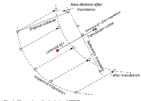
Feature 3: MTDT. Given an observed trajectory 𝑚 with 𝑛 sequences 𝑚 = {(𝑥1, 𝑦1), (𝑥2, 𝑦2) … , (𝑥𝑛, 𝑦𝑛)} and the set

of legitimate trajectories 𝐿, the 𝑀𝑇𝐷𝑇 between 𝑚 and 𝐿𝑖 is

calculated in three steps as follows:

1) Calculate the centroid point of 𝑚: 𝑚̅ = (𝑚̅̅̅̅, 𝑚𝑥 ̅̅̅̅)𝑦 as:

𝑚𝑥

̅̅̅̅ = 1

𝑛∑ 𝑥𝑘

𝑛

𝑘=1

𝑎𝑛𝑑 𝑚̅̅̅̅ =𝑦 1

𝑛∑ 𝑦𝑘

𝑛

𝑘=1

2) Let 𝐿𝑖 as one of the legitimate trajectories in L, assume

that 𝐿𝑖 has 𝑞 consecutive location data sequences: 𝐿𝑖= {(𝑥₁𝐿𝑖_{, 𝑦}

1 𝐿_𝑖

), (𝑥₂𝐿𝑖_{, 𝑦}

2 𝐿_𝑖

), … , (𝑥𝑞 𝐿_𝑖

, 𝑦𝑞 𝐿_𝑖

)}. We calculate the

minimum translation distance between m and 𝐿𝑖 as follows.

For every 𝐿𝑗_𝑖as a subset of 𝐿𝑖 with 𝑛 consecutive

observations 𝑗 = 1, 𝑞 − 𝑛 + 1̅̅̅̅̅̅̅̅̅̅̅̅̅̅̅ 𝐿𝑗_𝑖 = {(𝑥_𝑗𝐿𝑖_{, 𝑦}

𝑗 𝐿_𝑖

),

(𝑥_𝑗+1𝐿𝑖 _{, 𝑦}

𝑗+1 𝐿_𝑖

), … , (𝑥_{𝑗+𝑛−1}𝐿𝑖 _{, 𝑦}

𝑗+𝑛−1 𝐿_𝑖

)}.

2.1) Calculate the centroid point of 𝐿_𝑖𝑗: 𝐿𝑖 𝑗

̅ = (𝐿𝑖𝑥

𝑗 ̅̅̅̅_{, 𝐿}

𝑖𝑦 𝑗 ̅̅̅̅) as:

𝐿𝑗_𝑖𝑥

̅̅̅̅ =1

𝑛 ∑ 𝑥𝑘

𝐿𝑗

𝑗+𝑛−1

𝑘=𝑗

𝑎𝑛𝑑 𝐿̅̅̅̅ =𝑗_𝑖𝑦 1

𝑛 ∑ 𝑦𝑘

𝐿𝑗

𝑗+𝑛−1

𝑘=𝑗

2.2) Calculate the translation vector as:

𝑡̅ = (𝑡̅ , 𝑡𝑥 ̅ ) = (𝑚𝑦 ̅̅̅̅ − 𝐿𝑥 𝑖𝑥 𝑗

̅̅̅̅, 𝑚̅̅̅̅ − 𝐿𝑦 𝑖𝑦 𝑗 ̅̅̅̅)

2.3) Calculate 𝑚𝑡 (𝑚 after translation by 𝑡̅) as:

𝑚𝑡= {(𝑥1− 𝑡̅ , 𝑦𝑥 1− 𝑡̅̅̅̅, (𝑥𝑦) 2− 𝑡̅ , 𝑦𝑥 2− 𝑡̅ ), … , (𝑥𝑦 𝑛− 𝑡̅ , 𝑦𝑥 𝑛− 𝑡̅ )}𝑦

2.4) The translation distance 𝑑̅ between 𝑚 and 𝐿_𝑖𝑗 will be the distance between 𝑚𝑡 and 𝐿𝑖

𝑗

: 𝑑̅(𝑚,𝐿_𝑖𝑗) = 𝑑(𝑚𝑡, 𝐿𝑖 𝑗

).

2.5) After calculating all 𝑑̅(𝑚, 𝐿𝑗_𝑖), the minimum

translation distance between 𝑚 and 𝐿𝑖 will be:

𝑑̅𝑚𝑖𝑛(𝑚, 𝐿𝑖) = min{𝑑̅(𝑚, 𝐿𝑖 𝑗

)} ∀𝐿𝑗_𝑖∈ 𝐿𝑖 as a subset of 𝑛

consecutive observations in 𝐿𝑖.

3) The minimum distance between 𝑚 and 𝐿 will be calculated as:

𝑀𝑇𝐷𝑇(𝑚, 𝐿) = min{𝑑̅𝑚𝑖𝑛(𝑚, 𝐿𝑖)} ∀𝐿𝑖∈ 𝐿.

Fig. 1 illustrates the translation vector and the translation distance of two 5 − 𝑠𝑒𝑞𝑢𝑒𝑛𝑐𝑒 trajectories.

IV. EXPERIMENTAL SETUP

The VeReMi dataset has recently been published and is built specifically for testing location spoofing attacks in V2X scenarios [5]. The advantages of using the VeReMi dataset are (i) it presents different types of attackers; (ii) it simulates varied density conditions of vehicle network; (iii) it is consistent with its BSM’s broadcast rate; and (iv) the scenarios are conveniently labelled for using a machine learning approach. This section will describe VeReMi and

present the applications of our three designed features in machine learning for detecting and classifying attacks in this dataset.

A. Attacker Model

Attackers in VeReMi are assumed to be local, insider and active, and able to operate in both uniform and non-uniform areas [1]. A local attacker can only broadcast falsified information within their defined communication range, hence the damage created should be equally local. Attackers are also assumed to be insiders so that they can communicate with other vehicles regardless of the cryptographic defence used in communication. Attackers can be active, which means they can inject falsified information in the network the way they want. Finally, uniform areas (e.g. highway regions) refer to the areas where the travelling information of the attackers can be consistently transmitted to other vehicles, which is the opposite of non-uniform areas (e.g. rural areas).

B. Scenario and Attack Types

The VeReMi dataset comprises of 5 position forging attacks, 3 vehicle densities (low, medium and high), 3 attacker densities (10, 20 and 30 per cent) and each parameter set was repeated 5 times for randomization. The dataset contains the message logs of the attacking and benign

vehicles including reception time stamp, claimed

transmission time, claimed sender, unique message ID, GPS position (x, y, z), RSSI value, position noise and speed noise vector, for each receiving vehicle in every scenario. The

messages are broadcasted every second, so we chose 𝜀𝑡= 1

for trajectory extraction (see Definition 2). Along with that, a

Fig. 1. Illustration of calculating MTDT

TABLE I.VEREMI ATTACK TYPES DESCRIPTION [1]

Type Details Parameters

T1 Constant Attacker transmits a fixed _location x = 5560 y = 5820

T2

Constant Offset

Attacker transmits a fixed, offset added to the real position

∆x = 250 ∆y = -150

T4

Random Attacker sends a random position inside the simulation area

Uniformly random in playground

T8

Random Offset

Attacker sends a random position in a rectangle around the vehicle

∆x, ∆y are uniformly random in [-300, 300]

T16

Eventual Stop

Attacker behaves normally for some time and then attacks by transmitting the same position repeatedly

ground truth file is also maintained which records the true values of the BSM attributes of both attacker and benign vehicles. The attacker type attribute in the Ground Truth file keeps the label of the attack ID as described in Tab. I.

C. Machine Learning Designs

Given an 𝑛 − 𝑠𝑒𝑞𝑢𝑒𝑛𝑐𝑒 trajectory for inspection, it can be legitimate (referred as 𝑇0) or one of five types of attacks (referred as 𝑇1, 𝑇2, 𝑇4, 𝑇8, 𝑇16). The purposes of our designed features in detecting and classifying the attacks are as follows.

𝑀𝑃𝐶 aims at classifying 𝑇1 and 𝑇16 from other attacks. We have 𝑀𝑃𝐶(𝑇0, 𝑇2, 𝑇4, 𝑇8) = 0 because 𝑘𝑖= 0 ∀𝑖. On

the other hand, 𝑇1 report constant location all the time,

therefore 𝑘𝑖= 𝐾 ∀𝑖, so 𝑀𝑃𝐶(𝑇1) = 𝐾. Meanwhile, for

𝑇16, there should be at least one 𝑖 so that 𝑘𝑖= 0 to indicate

the time when attackers transform from normal state to attack state; while there should be at least one 𝑗 that 𝑘𝑗= 𝐾 to

reflect the attack. Therefore, we have 𝐾

𝑛−1≤ 𝑀𝑃𝐶(𝑇16) ≤

𝐾(𝑛−2)

𝑛−1 (1). Our experiments show that choosing a small K

may lower the performance of KNN and SVM as the classification distances will become too small. In this work, we select 𝐾 = 1000.

When 𝑇1 and 𝑇16 are detected, 𝑀𝐷𝑇 will help to differentiate 𝑇0 from the remaining types 𝑇2, 𝑇4, 𝑇8 because

𝑀𝑇𝐷(𝑇0) values should be close to 0 as normal trajectories

should find similar moving patterns in the legitimate set. On

the other hand, 𝑀𝐷𝑇(𝑇2, 𝑇4, 𝑇8) values should be large due

to the small chance of having similar movement patterns. Moreover, 𝑀𝐷𝑇 can help to classify 𝑇4 from others because

the 𝑀𝐷𝑇(𝑇4) values are much larger compared with 𝑀𝐷𝑇

of other types.

Our experiments show that 𝑀𝑇𝐷(𝑇2) and 𝑀𝑇𝐷(𝑇8)

values are close, therefore 𝑀𝑇𝐷 alone cannot help to differentiate between 𝑇2 and 𝑇8. Therefore, we design 𝑀𝑇𝐷𝑇 for further classifying these two types. As 𝑇2 is translated from a legitimate trajectory, 𝑀𝑇𝐷𝑇(𝑇2) values should be close to 0. Meanwhile, 𝑀𝑇𝐷𝑇(𝑇8) values will remain large due to the small chance of having movement pattern which is similar to a translated legitimate trajectory.

With the three features, we implemented similar machine learning algorithms (i.e. 𝐾𝑁𝑁 and 𝑆𝑉𝑀) with [1] for

comparison. In details, the 𝐾𝑁𝑁 was done using the

MATLAB built-in function 𝑓𝑖𝑡𝑐𝑘𝑛𝑛 with Euclidean distance

to compute the nearest neighbour. The number of nearest neighbours 𝐾 was tuned from 1-100, while 𝐾 with the highest correct-classification-rate (CCR) was chosen as the best 𝐾 for prediction model. For 𝑆𝑉𝑀, instead of using the binary classification 𝑓𝑖𝑡𝑐𝑠𝑣𝑚 function as presented in [1], we use the 𝑓𝑖𝑡𝑐𝑒𝑐𝑜𝑐 function which allow to classify for more than two types of attacks. We also use 𝑓𝑖𝑡𝑐𝑒𝑐𝑜𝑐 in binary classification as our experiments show that it always performs better than the 𝑓𝑖𝑡𝑐𝑠𝑣𝑚.

D. Parsed Dataset and Feature Extractions

The VeReMi dataset provides results of 225 simulations, 45 for each type of attacks. We selected 80% of the data for training while the remaining 20% are used for testing. For each type of attack, 36 sets of simulation logged data were chosen randomly to include in the training data, while the remaining 9 logged results are included in the testing data.

We extracted all the unique legitimate trajectories from the 80% training dataset into a database. We assume that this database will be maintained by a central authority, where the vehicles can send their suspected observations to for querying and getting the judgement. We also extract the three features for every 𝑛 − 𝑠𝑒𝑞𝑢𝑒𝑛𝑐𝑒 trajectory in the training dataset to build the machine learning models. Notes that to calculate the 𝑀𝑇𝐷 and 𝑀𝑇𝐷𝑇 of a trajectory, this trajectory will be excluded from the legitimate database to avoid any duplication. Finally, for testing, for every 𝑛 −

𝑠𝑒𝑞𝑢𝑒𝑛𝑐𝑒 trajectory in the 20% testing dataset, we calculate

its three features based on the extracted legitimate database to query with the detection and classification models. The behaviour labels of the trajectory will be used to verify the accuracy performance of the models.

E. Inspection Length Consideration

To apply our approach, we need all the three features to be valid for all inspected trajectories. It is obvious that 𝑀𝑃𝐶(𝑇16) is invalid when 𝑛 = 1 or 𝑛 = 2 according to (1). Therefore, the minimum value of 𝑛 to be considered in this paper is 3. As 𝑛 will influence all the values of the three features significantly, we vary 𝑛 from 3 to 10 to study its impacts. Notes that when judging the behaviours of a suspected vehicle, if the central authority can gather observations from all other vehicles, 𝑛 can be very large as desired. However, if the observations come from a single source, 𝑛 is not likely to be too large as the suspected vehicle may move out from the communication coverage of the source, which break the continuity of the observations.

F. Evaluation Metrics

The detection performance of the approach can be evaluated through the precision and recall. Firstly, each prediction result will be counted in one of the four following categories: True Positive (TP): detect an attacker as an attacker; False Positive (FP): detect a legitimate observation as an attacker; False Negative (FN): detect an attacker as a

legitimate vehicle; and True Negative (TN): detect a

legitimate observation as legitimate. The precision is calculated as 𝑇𝑃

𝑇𝑃+𝐹𝑃, while the recall is calculated as

𝑇𝑃

𝑇𝑃+𝐹𝑁.

We also formulate a confusion matrix to see the performance of the classification.

V. RESULTS AND DISCUSSIONS

We evaluate our approach in a similar way to the evaluations in [1]. Firstly, we evaluate the detection for each type of attacks by combining only the corresponding attack data and the normal data to use in training and testing. For example, to evaluate the detection of 𝑇2, we keep only 𝑇2 and normal data in the training and testing dataset while excluding all other attack types. Secondly, we evaluate the overall performance in differentiating between attacks and non-attacks by generalise the attack type, which means that all the attack label 1, 2, 4, 8, 16 will be relabelled as 1. Lastly, we evaluate the classification performance for the original labelled attack dataset in two cases: with and without the normal behaviours. Notes that authors in [1] avoided the evaluation of classifications when normal behaviours were included due to unbalance dataset which led to poor performance.

A. Detection per Attack Type

our approach. As can be seen in the figure, our approach achieved near 100% in precision and recall for

𝑇1, 𝑇4, 𝑇8, 𝑇16 when applying either 𝐾𝑁𝑁 or 𝑆𝑉𝑀. The

𝑀𝑃𝐶 feature will always be 1000 if a trajectory is 𝑇1, and

always be 0 if it is normal. For 𝑇16, 𝑀𝑃𝐶 have a minimum

value of 111 and maximum value of 888, both when

inspecting with 10 sequences. Therefore, 𝑀𝑃𝐶 can be

considered as a plausibility check for both 𝑇1 and 𝑇16 to achieve accurate detections. On the other hand, 𝑇4 and

𝑇8 trajectories will have much larger 𝑀𝑇𝐷 and 𝑀𝑇𝐷𝑇

values than the normal trajectories (most of 𝑀𝑇𝐷(𝑇4) and 𝑀𝑇𝐷𝑇(T4) values are larger than 1000; most of 𝑀𝑇𝐷(𝑇8)

and 𝑀𝑇𝐷𝑇(T8) values are larger than 100 and much smaller

than 1000; while most of other 𝑀𝑇𝐷(𝑇0) and 𝑀𝑇𝐷𝑇(𝑇0)

are smaller than 20), therefore it is not difficult to detect these attacks.

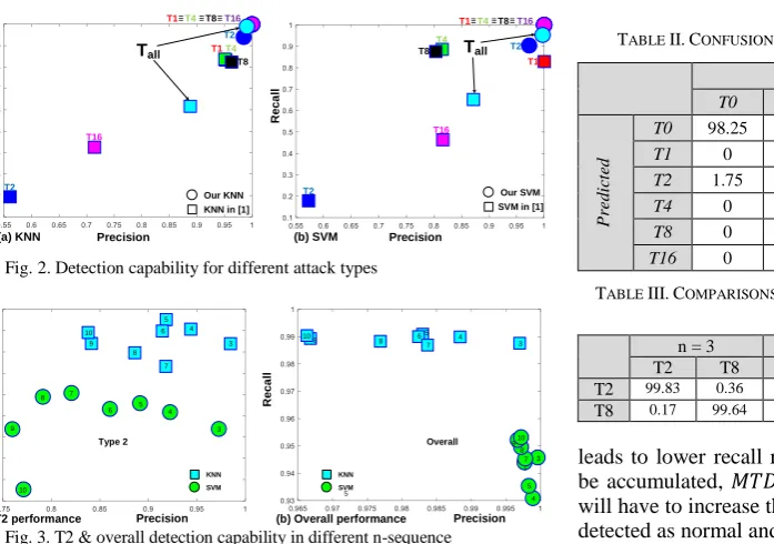
For 𝑇2, we achieved much better precisions (the best rate is 98.5% for KNN with 3-sequence) and recalls (94% for KNN with 3-sequence) compared to [1]. [1] has low performance because it does not have any feature that can separate 𝑇2 from normal performance. Meanwhile, in our approach, the 𝑀𝑇𝐷 is specifically designed to separate 𝑇2

from normal performance. Fig. 3a shows 𝑇2 detection

capability with different 𝑛 sequence when applying KNN and SVM. It can be seen that in general when 𝑛 increase, the precision rates decrease significantly while the recall rates increase slightly. Notes that unlike other verification approaches, we do not try to predict the accurate locations of the trajectories. Instead of that, we try to find the minimum deviation of the reported trajectories compared with the normal patterns. A small 𝑛 is expected to create small

accumulated deviations, hence lead to smaller 𝑀𝑇𝐷(𝑇0)

margin (upper bound values are at about 50 when 𝑛 ≤ 5 and about more than 150 when 𝑛 > 5). On the other hand, statistics of 𝑀𝑇𝐷(𝑇2) are not affected much by 𝑛, because the deviations are always high. Therefore, when 𝑛 is small, the models may create better separations between normal and attack dataset, which lead to higher precision. However, the smaller margin will make the model more sensitive, so the

𝑀𝑇𝐷(𝑇0) outliers will likely be detected as attacks, which

leads to lower recall rates. When 𝑛 is large, deviations will be accumulated, 𝑀𝑇𝐷(𝑇0) will be increased so the models will have to increase the margin, which makes more 𝑇2 to be detected as normal and decrease the precisions. Nevertheless,

the 𝑀𝑇𝐷(𝑇0) outliers will less likely be detected as attacks,

which make the recall rates increase slightly.

B. Overall Detection Performance

For evaluations in detecting attacks in general (all attacks are re-labelled as 1), Fig. 2 shows the comparisons between our approach and [1], while Fig. 3b presents the comparisons between using KNN and SVM with different length of inspected trajectories in our approach. As can be seen from the figures, our approach shows significant better performances than [1], while there are always trade-offs between the precision and recall rates when choosing different inspection length. With KNN, our approach got a precision rate of 99.7% (𝑛 = 3), which decreases gradually to 96.84 (𝑛 = 10), whilst the recall rates are around 99%. When using SVM fitcecoc, the precision rates are always larger than 99.7%, however, the recall rates are ranging from

93.2% (𝑛 = 4) to 95.2% (𝑛 = 10). On the other hand, when

using the SVM fitcsvm, the precision rate is highest at 98.7%

(𝑛 = 3), which decrease gradually to 88.77% (𝑛 = 10),

while the recall rates are around 99%. As the model show very good performance when detecting 𝑇1, 4, 8, 16, the main misdetections should come from 𝑇2, so the explanations will be similar to these of Section V.B.

C. Classification Performance

Tab. II shows the confusion matrix of best CCR performance in classification over all the implementations, which is 𝐾𝑁𝑁 with 𝑛 = 6, 𝑘 = 97. As can be seen, 𝑇2 is the most difficult attack to classify, which was detected as normal in 6.39% of the cases. For all the experiments, the overall misclassification rates are always lower than 4.7%.

When 𝑇0 are removed from the dataset, our models classify correctly 𝑇1, 𝑇4, and 𝑇16 in most of the cases. The main confusions are those between 𝑇2 and 𝑇8. Tab. III

shows the confusion matrix between 𝑇8 and 𝑇2 when using

the SVM fitcecoc. Our approach achieved small

misclassified rates at less than 0.6%, which is a significant

improvement from [1] where about 20% of 𝑇2 are

misclassified as 𝑇4 or 𝑇8. The confusion rates also decrease

when 𝑛 increase. 𝑀𝑇𝐷𝑇 is the main reason for this

improvement. As 𝑇2 is a translated form of a legitimate

T1 T2 T4 T8 T16 Tall

KNN in [1]

Our KNN T2

T16

T1 T16

T1T4 T8

T8 T1 T4 Precision Precision Re c a ll R e c a ll

SVM in [1] Our SVM

T2 T2

T16

T1T4 T8

Tall

(a) KNN (b) SVM

Fig. 2. Detection capability for different attack types

10 8 7 65 3 4 10 6 5 8 7 9 3 4 5 6 7 8 9 10 10 3 4 5 6 7 8 9 R e c a ll R e c a ll Precision Precision KNN SVM KNN SVM

Type 2 Overall

3 4

5 9

(a) T2 performance (b) Overall performance

Fig. 3. T2 & overall detection capability in different n-sequence

TABLE II.CONFUSION MATRIX OF BEST CCRKNN(N=6, K=97)(%)

Ground Truth

T0 T1 T2 T4 T8 T16

Pre

d

ic

te

d

T0 98.25 0 6.39 0 0 0

T1 0 100 0 0 0 0

T2 1.75 0 93.61 0 0.04 0

T4 0 0 0 100 0 0

T8 0 0 0 0 99.96 0

T16 0 0 0 0 0 100

TABLE III.COMPARISONS OF CONFUSION RATES (%) BETWEEN T2 AND T8

(SVM- FITCECOC)

n = 3 n = 4 n = 5 n ≥ 6

T2 T8 T2 T8 T2 T8 T2 T8

T2 99.83 0.36 99.9 0.3 99.94 0.01 1 0

trajectory, 𝑀𝑇𝐷𝑇(𝑇2) value should be small. Meanwhile,

𝑀𝑇𝐷𝑇(𝑇8) values should be much larger than 𝑀𝑇𝐷𝑇(𝑇2)

because 𝑇8 will have high deviations from any translated trajectories. These deviations will also be accumulated to be higher when 𝑛 increases, which helps to classify between 𝑇2 and 𝑇8 better.

D. Inspection Length Considerations

As can be seen from previous discussions, a small 𝑛 can give high precision rates in most of the cases, however, the prediction models will be more sensitive, which leads to lower recall rates. Moreover, too small 𝑛 can also lead to misclassification between 𝑇2 and 𝑇8. On the other hand, a large 𝑛 provides high recall rates and help to classify the attacks correctly. However, it will also decrease the precision rates significantly, not mention that in reality, long observations of the suspected vehicles are more difficult to achieve. Therefore, for a balance between the detection and classification capability and the potential to apply in real life scenarios, the recommended value of n to choose is 5.

VI. CONCLUSION

In this paper, we introduced three novel features

extracted from an 𝑛 − 𝑠𝑒𝑞𝑢𝑒𝑛𝑐𝑒 trajectory for use in

machine learning models to detect and classify misbehaviour attacks. We implemented these features in KNN and SVM and compared them to a previous approach that used different features. We evaluated the detection performance of our models using the VeReMi dataset and achieved overall precision of up to 99.7% while maintaining a recall in excess of 99%. The classification accuracy also outperforms the previous best obtained results with less than a 4.7% misclassification rate. Moreover, by studying the impacts of observation length on our models’ performance, we showed that our approach can provide reliable judgements even after as few as 3 observations (i.e. 3 seconds), which suggests that they can be useful for near real-time detection and classification. In the future, we aim to extend the attack

models (e.g. adding more sophisticated types of

misbehaviours) and improving the attack detection techniques to be able to detect and classify more types such as Sybil, replay, or stealthy attacks.

ACKNOWLEDGEMENT. This work was funded by UK Research and Innovation through INNOVATE UK in project CAPRI (TS/P012264/1).

REFERENCES

[1] S. So, P. Sharma, and J. Petit, "Integrating Plausibility Checks and Machine Learning for Misbehavior Detection in VANET," in 2018 17th IEEE International Conference on Machine Learning

and Applications (ICMLA), 2018, pp. 564-571.

[2] C. Maple, "Security and privacy in the internet of things," Journal of Cyber Policy, vol. 2, no. 2, pp. 155-184, 2017/05/04 2017.

[3] R. W. v. d. Heijden, A. Al-Momani, F. Kargl, and O. M. F. Abu-Sharkh, "Enhanced Position Verification for VANETs Using Subjective Logic," in 2016 IEEE 84th Vehicular Technology

Conference (VTC-Fall), 2016, pp. 1-7.

[4] R. W. v. d. Heijden, S. Dietzel, T. Leinmüller, and F. Kargl, "Survey on Misbehavior Detection in Cooperative Intelligent Transportation Systems," IEEE Communications Surveys & Tutorials, vol. 21, no. 1, pp. 779-811, 2018.

[5] R. W. van der Heijden, T. Lukaseder, and F. Kargl, "VeReMi: A Dataset for Comparable Evaluation of Misbehavior Detection in VANETs," Cham, 2018, pp. 318-337: Springer International Publishing.

[6] C. Sommer, R. German, and F. Dressler, "Bidirectionally Coupled Network and Road Traffic Simulation for Improved IVC Analysis," IEEE Transactions on Mobile Computing, vol. 10, no. 1, pp. 3-15, 2011.

[7] H. Stübing, J. Firl, and S. A. Huss, "A two-stage verification process for Car-to-X mobility data based on path prediction and probabilistic maneuver recognition," in 2011 IEEE Vehicular

Networking Conference (VNC), 2011, pp. 17-24.

[8] C. Yavvari, Z. Duric, and D. Wijesekera, "Vehicular dynamics based plausibility checking," in 2017 IEEE 20th International Conference on Intelligent Transportation Systems (ITSC), 2017, pp. 1-8.