Quantum Theory of Sensing and
Thermoelectricity in Molecular
Nanostructures
Qusiy Hibeeb Hityhit Al-Galiby
B.Sc, M.Sc.
Department of Physics, Lancaster University, UK
Ph.D. Thesis
This thesis is submitted in partial fulfilment of the requirements
for the degree of Doctor of Philosophy
I
Declaration
Except where stated otherwise, this thesis is a result of the author's original work and has not been submitted in whole or in part for the award of a higher degree elsewhere. This thesis documents work carried out between June 2012 and March 2016 at Lancaster University, UK, under the supervision of Prof. Colin J. Lambert and funded by UK EPSRC grants EP/K001507/1, EP/J014753/1, EP/H035818/1, the European Union Marie-Curie Network MOLESCO 606728, the Ministry of Higher Education and Scientific Research (MOHESR) in Iraq, Al Qadisiyah University and the Ministry of the Presidency of Iraq, Establishment of Martyrs.
II
Abstract
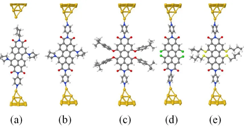
This thesis presents a series of studies into the electronic and thermoelectric properties of molecular junction single organic molecules: They include perylene Bisimide (PBIs),
naphthalenediimide (NDI), metallo-porphryins and a large set of symmetric and asymmetric molecules.
Two main techniques will be included in the theoretical approach, which are Density Functional Theory, which is implemented in the SIESTA code [1], and the Green’s function formalism of elctron transport (Chapter 2), which is implemented in the GOLLUM code [2], it is a next-generation code, born out of the non-equilibrium transport code SMEAGOL code [3]. Both techniques are used to extensively to study a family of perylene bisimide
molecules (PBIs) (Chapter 3) to understand the potential of these molecules for label-free sensing of organic molecules by investigating a change in the electronic properties of PBI derivatives. Also, these techniques are used to simulate electrochemical gating of a single molecule naphthalenediimide (NDI) junction (Chapter 4) using a strategy to control the number of electrons on the molecule by modelling different forms of charge double layers comprising positive and negative ions.
Chapter 5 will deal with the thermoelectric properties of the single organic molecule. I will demonstrate that varying the transition metal-centre of a porphyrin molecule over the family of metallic atoms allows the molecular energy levels to be tuned relative to the Fermi energy of the electrodes and that leads to the ability to tune the thermoelectric properties of metallo-porphryins.
III
IV
Acknowledgments
Nothing would have been completed in this thesis without the collaboration, the help and guidance of many people. All my gratitude goes to my supervisor Prof. Colin J. Lambert for his continuous guidance and the intensive fruitful discussion over these years. I would like to thank Dr. Steve Baily, Dr. Iain Grace for thier contniuos support.
I would like also to thank my sponsor, the Ministry of Higher Education and Scientific Research (MOHESR) in Iraq, Al Qadisiyah University and the Ministry of the Presidency of Iraq, Establishment of Martyrs for funding my PhD study.
I would like to thank the collaborating experimental groups, Prof. Thomas Wandlowski and Prof. Wenjing Hong from Bern University for their successful experiments. I would like to thank all my friends and colleagues in Colin’s group, especially Hatef Sadeghi, Dr. David Manrique, Dr. Laith Algharagholy, Dr. Thomas Pope, Dr. Amaal Al-Backri, Mohammed Noori, Nasser Almutlaq, Zain Al-Milli, Sara Sangtarash and Elaheh Mostaani.
To the martyrs of Iraq and in particular my brother, the martyr Saleh Hibeeb Al-Galiby, you are my inspiration in life, eternal bliss to you. My dear father, thank you so much for your great kind, and my brother Dr. Hayder, thank you for your great efforts, mercy and paradise to you.
V
List of Publications
1. Al-Galiby, Qusiy, Iain Grace, Hatef Sadeghi, and Colin J. Lambert. "Exploiting the extended π-system of perylene bisimide for label-free single-molecule sensing." Journal
of Materials Chemistry C 3, no. 9 (2015): 2101-2106.
2. Li, Yonghai, Masoud Baghernejad, Al‐Galiby Qusiy, David Zsolt Manrique, Guanxin Zhang, Joseph Hamill, Yongchun Fu et al. "Three‐State Single‐Molecule Naphthalenediimide Switch: Integration of a Pendant Redox Unit for Conductance
Tuning." Angewandte Chemie International Edition 54, no. 46 (2015): 13586-13589.
3. Al-Galiby, Qusiy H., Hatef Sadeghi, Laith A. Algharagholy, Iain Grace, and Colin Lambert. "Tuning the thermoelectric properties of metallo-porphyrins."Nanoscale 8, no. 4 (2016): 2428-2433.
1
Contents
1. Introduction ……….. 4
1.1 Molecular Electronics (ME) ………... 1.1.1 Perylene Bisimide (PBIs) ……… 1.1.2 Naphthalenediimide (NDI) ………. 1.1.3 Porphyrin ………
4 6 7 8
2. Theory of Quantum Transport ……… 9
2.1 The Landauer formula ……… 2.2 Thermoelectric coefficients ……….
2.2.1 Generalized formula for the thermoelectric coefficients ………… 2.3 Scattering Theory ……… 2.3.1 One dimensional (1-D) linear crystalline lattice ……… 2.3.2 One dimensional (1-D) scattering ……….. 2.4 Generalization of the Scattering Formalism ………..
2.4.1 A doubly infinite Hamiltonian and Green’s function of the electrodes ………. 2.4.2 Effective Hamiltonian of the Scattering Region ……… 2.4.3 Scattering Matrix ……… 2.5 Calculation in Practice ………... 2.6 Features of the Transport Curve ……… 2.6.1 Breit-Wigner Resonance ………. 2.6.2 Fano Resonances ……… 2.6.3 Anti-Resonances ……….
2
2.7 Hamiltonian used in the thesis ……….. 46
3. Single-Molecule Sensing of Perylene Bisimide ……….. 48
3.1 Single-Molecule Conductance of Perylene Bisimide (PBIs) ………... 3.1.1 Motivation ………. 3.1.2 Computational Methods ……… 3.1.2.1 Molecular junction and the conductance ………. 3.1.3 Results and discussion ……….. 3.1.3.1 Locating the optimal value of EF ………
3.2 Exploiting the Extended π-System of Perylene Bisimide for Label-free Single-Molecule Sensing ……… 3.2.1 Motivation ………. 3.2.2 Molecular Complexes ……….. 3.2.3 Molecular junction and the conductance ………. 3.2.4 Evaluating of error in the currents for a distribution of geometries. 3.2.5 Fluctuation positions of the analytes above the PBIs backbone… 3.2.6 Quantifying the sensitivity of the PBIs for discriminating sensing. 3.3 Summary ……….
48 48 49 51 53 54 56 56 59 63 70 70 78 80
4. Three States Single-Molecule Naphthalenediimide Switch: Integration of Pendant Redox Unit for Conductance Tuning ………. 4.1 Introduction ……….. 4.2 Experimental work ………... 4.2.1 Single-molecule break junction experiments ……….. 4.2.2 Further analysis of NDI-D conductance measurement………… 4.3 Theoretical Method ………...
4.3.1 The junction and Charge double layer geometries ………..
3
4.4 Results and discussion ……….. 4.5 Summary ………
92 97
5. Tuning the thermoelectric properties of metallo-porphyrins ………. 98
5.1 Motivation ……….. 5.2 Introduction ……… 5.3 Methods ……….. 5.4 Results and Discussion ………..
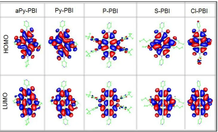
5.4.1 Plots of frontier orbitals and spin-dependent transmission coefficients ……….. 5.4.2 Thermoelectric properties of Fe(III)-porphyrin in presence of a Cl counter anion ……….. 5.4.3 The calculation of Mn-porphyrin in presence of (Cl) …………. 5.5 Summary ………
98 100 101 103 110 118 121 124
6. A New Approach to Materials Discovery for Electronic and Thermoelectric Properties of Single-Molecule Junctions ……… 6.1 Introduction ……… 6.2 Methods ……….. 6.3 Results and discussion ………... 6.4 Associated Content ……… 6.5 Summary ……….
125 126 129 132 143 164
7. Conclusion ………. 165
4
Chapter 1
Introduction
1.1 Molecular Electronics
In recent decades technological advances have accelerated at a rapid pace, partially due to the ever increasing need for the miniaturization of electronic devices. Whether the progress of research and development will be able to help this need in the future depends on how much we can further extend our computational capabilities through nanotechnology.
In the mid-1960s, Gardon Moor observed that the number of transistors per unit area on a chip was doubling approximately once every two years [1]. The size of the current silicon based transistors are now down to only tens of nanometers, where he expected that this trend could continue for only a 10-year long period, nearly half a century later, the exponential growth continues. However, if Moore's law is to continue, the transistors will have to shrink to the atomic scale within twenty years and enter the field of sub-10 nm nanoelectronics. One important branch of this field, that this thesis is focused on, is molecular electronics
5
fast and cheap, with lower power consumption. Therefore, single molecule devices are very appealing candidates for future applications.
So far, theoretical and experimental studies have focused on electrode-molecule-electrode (EME) junctions, which will be discussed in this thesis. The main experiment techniques to study these systems are Scanning Tunnelling Microscopy Break Junctions (STM-BJ) [2, 3] and Mechanically Controllable Break Junctions MCBJ [4, 5]. Using such break junctions, a third electrode can be also introduced by chemical gating [6, 7].
A simplistic picture of the physics of such the molecules in EME contacts is that they are a kind of quantum dot, because they are small finite sized objects and have discrete electronic spectra and single-electron charging energies reaching the electron-volt range. However, molecules are more than “just” quantum dots. The word “dot” carries with it the impression of a relatively structureless, even quasi-zero-dimensional object. Yet, the long-term goal of molecular electronic (ME) is precisely to take the advantages of the endless variability of chemical compounds to design molecules having just the right properties for use as single-molecule electronic components. Furthermore single-molecules can have multiple conformations and they could be used as rectifiers [8]. Indeed Aviram and Ratner proposed theoretically the first molecular rectifier and their suggestion was the starting point for the development of this field. Molecular electronics also could be used in a wide range of applications such as switches [9] and sensors [10, 11].
6
The ability to manage waste heat is a major challenge, which currently limits the performance of information technologies. To meet this challenge, there is a need to develop novel materials and device concepts, innovative device architectures, and smart integration schemes, coupled with new strategies for managing and scavenging on-chip waste heat. The development of new high-efficiency and low-cost thermoelectric materials and devices is a major target of current research. Thermoelectric materials, which allow highly-efficient heat-to-electrical-energy conversion from otherwise wasted low-level heat sources, would have enormous impact on global energy consumption.
Nanoscale systems and especially nanoscale structures are very promising in this respect, due to the fact that transport takes place through discrete energy levels. The ability to measure thermopower in nanoscale junctions opens the way to developing fundamentally-new strategies for enhancing the conversion of heat into electric energy [19]. The thermoelectric properties of materials will be discussed in this thesis.
Therefore one aim of this thesis is to provide rules for the discovery of new materials by
predicting electronic [20] and thermoelectric properties of molecules. This is particularly
important, because theoretical methods such as density functional theory and GW many
body theory do not usually provide quantitative predictions of such properties.
1.1.1 Perylene bisimide (PBIs)
7
electronic properties and their industrial applications as dyes and pigments [8, 23]. Their unique properties are primarily derived from their large extended systems, which in π-stacked arrays lead to a variety of intermolecular π-orbital overlaps for the different derivatives [31]. Furthermore their high electron affinities, large electron mobilities, chemical and thermal stabilities, and variety of functional forms with different bay-area substituents has led to their widespread use in organic solar cells [32-35], organic field-effect transistors (OFETs) [36, 37] particularly as n-type materials [38, 39], and organic sensors [40-47].
Figure 1.1: shows the chemical structure of Perylene Bisimide (PBIs) molecule.
The chemical structure of perylene bisimide (Figure 1.1) involves two glutarimide groups with two naphthalenes (which is called perylene). The core of perylene bisimide can be functionalized in different ways by varying both the bay and ortho positions [23].
1.1.2 Naphthalenediimide (NDI)
The second class of molecular function are formed from naphthalene diimide (NDI), which has attracted much attention in organic electronics [48-50] and the supramolecular chemistry [51] community acting as an electron acceptor with n-type semiconductor characteristics. This molecule is studied in chapter 4 and comprises of a pyrene core with two alkyl chains
Ortho
8
in the bay-area position and benzothiophenes (DBT) as anchor groups as shown in Figure 1.2.
Figure 1.2: shows the chemical structure of naphthalenediimide (NDI) molecule.
1.1.3
Porphyrin
Finally I investigate functions formed from porphyrins, which are attractive as building blocks for molecular-scale devices, because they are conjugated, rigid, chemically stable and form metalloporphyrins by coordinating a variety of metallic ions [52-60]. The porphyrin molecule comprises of a four pyrrole cores (the inner ring π-system), whereas the metallo-porphryin involves a four pyrrols cores with a metallic atom χ in the centre of the molecule as shown in Figure 1.3 (a and b). Typical example of χ are zinc, copper, nickel and various others.
Figure 1.3: (a and b) illustrate the chemical structure of porphryin and metallo-porphryin molecules, respectively.
χ
9
Chapter 2
Theory of Quantum Transport
One of the important challenges in molecular electronic how to connect the molecule to metallic or any other electrodes to probe its electronic properties. For the molecular system, the contacts between the molecule and the electrodes are usually a significant part which determines the electronic properties in addition to the molecular properties. This contact involves scattering processes from the electrode to the molecule and from the molecule to the electrode. A system like this is not periodic, so a band structure is no longer sufficient to describe its electronic properties. For this reason a general approach is required to understand and calculate the scattering processes between the electrodes that are interconnected with a molecule.
10
2.1 The Landauer formula
The standard way to describe transport phenomena the phase-coherent mesoscopic systems is by evaluating the Landauer formula [61, 62]. The applicability of the method holds for phase coherent systems, in other words where a single wave function of fixed energy is sufficient to describe the electronic flow. For a mesoscopic sample the relation between the electrical conductance and the transmission properties of electrons passing through this sample can be described by the Landauer formula, which is the key formula that translates the theoretical electron transmission probability calculations obtained from the scattering formalism to the experimental quantities, such as the conductivity or the current.
Our starting point begins by considering a mesoscopic scatterer connected to two electron reservoirs (or contacts) by means of two ideal ballistic leads as shown in Figure 2.1. All inelastic relaxation processes are limited to the reservoirs [63]. The reservoirs have slightly different chemical potentials 𝜇𝐿− 𝜇𝑅 > 0, which will drive electrons from the left to the right reservoir. Initially, I will discuss the solution for one open channel (i.e. where only one electron is allowed to travel in a given direction).
Figure 2.1: illustrates a mesoscopic scatterer connected to contacts by ballistic leads. The µL and µR
11
To calculate the current in such a system we start by analyzing the incident electric current,
𝛿𝐼, generated by the chemical potential gradient:
L R
E
n
ev
I
(2.1.1)where e is the electronic charge, v in the group velocity and n/Eis the density of states
per unit length in the lead in the energy window defined by the chemical potentials of the contacts:
v
k
n
E
k
k
n
E
n
1
(2.1.2) In one dimension, after including a factor of 2 for spin dependency, n/k1/ . By substituting this into Eq. 2.1.2 we find thatn/E1/v. This simplifies Eq. 2.1.1 to:
V
h
e
h
e
I
L
R
2
2
2 (2.1.3)where V is the voltage generated by the potential mismatch. From Eq. 2.1.3, it is clear that in the absence of a scattering region, the conductance of a quantum wire with one open channel is 2e2/h, which is approximately 77.5 S(or in other words, a resistance of 12.9
K ). This is reasonable quantity; it typically appears on the circuit boards of everyday electrical appliances.
Now if we consider a scattering region, the current collected in the right contacts will be:
h
e
G
V
I
V
h
e
I
22
2
12
This is widely-known Landauer formula, relating the conductance, G, of a mesoscopic scatterer to the transmission probability,
of the electrons traveling through it. It describes the linear response conductance, hence it only holds for small bias voltages,V 0.For the case of more than one open channel, the Landauer formula has been generalized by Büttiker [62], where the transmission coefficient is replaced by the sum of all the transmission amplitudes describing electrons incoming from the left contact and arriving to the right contact. The Landauer formula Eq. (2.1.3) for many open channels hence becomes:
† 2 2 , , 2 2 2 tt Tr h e t h e G V I j i j i
(2.1.5)Where ti,j is the transmission amplitude describing scattering from jth channel of the left electrode to the ith channel of the right electrode. Similarly, the reflection amplitudes ri,j which describe scattering processes where the particle is scattered from the jth channel of the left electrode to the ith channel of the same electrode. By combining the reflection and transmission amplitudes, one obtaining the matrix which connects states coming from the left lead and vice versa, this object is called the S matrix:
r
t
t
r
S
(2.1.6)13
2.2 Thermoelectric coefficients
In the linear-response regime, the electric current I and heat current 𝑄̇ passing through a device is related to the voltage difference ∆𝑉 and temperature difference ∆𝑇 by Buttiker, Imry, Landauer, et al. [62, 65-67]. Therefore both currents are related to the temperature and potential differences through the thermoelectric coefficients G, L, M, and K [68, 69]
(𝑄̇) = (𝐼 𝐺 𝐿
𝑀 𝐾) (∆𝑉∆𝑇) (2.2.1)
The thermoelectric coefficients L and M, in the absence of a magnetic field, are related by an Onsager relation
𝑀 = −𝐿𝑇 .
where T is temperature . By rearranging these equations, the current relations in terms of the measurable thermoelectric coefficients: electrical resistance R = 1/G, thermopower
𝑆 = −∆𝑉/∆𝑇, Peltier coefficients Π and the thermal conductance 𝑘 can be expressed
(Δ𝑄̇V) = ( 1
𝐺 −
𝐿 𝐺 𝑀
𝐺 𝐾 −
𝐿𝑀 𝐺
) ( 𝐼∆𝑇) = ( 𝑅 𝑆
Π −𝑘) ( 𝐼∆𝑇) (2.2.2)
The thermopower S is defined as the potential drop due to a temperature difference in the absence of an electrical current
𝑆 ≡ − (∆𝑉 ∆𝑇)𝐼=0 =
𝐿
𝐺, (2.2.3)
the Peltier coefficient Π is defined as the heat transferred purely due to the charge current in the absence of a temperature difference
Π≡ (𝑄̇
𝐼)∆𝑇=0 = 𝑀
14
and the thermal conductance 𝑘 is defined as the heat current due to the temperature drop in the absence of an electric current
𝑘 ≡ − (𝑄̇
∆𝑇)𝐼=0 = −𝐾 (1 + 𝑆2𝐺𝑇
𝐾 ), (2.2.5)
Therefore the evaluation of S or Π gives an idea of how well the device will act as a heat driven current generator or a current driven cooling device.
An additional quantity, the thermoelectric figure of merit, ZT [70, 71] can also be defined in terms of these measurable thermoelectric coefficients
𝑍𝑇 = 𝑆2𝐺𝑇
𝑘 . (2.2.6)
From classical electronics, ZT is derived by finding the maximum induced temperature difference produced by an applied electrical current in the presence of Joule heating. Let's consider a current carrying conductor placed between two heat baths with temperatures
TL and TR, and electrical potentials VL and VR respectively. The thermoelectric figure of
merit can be defined by finding the maximum induced temperature difference of the conductor due to an electrical current. Defining 𝑄̇ as the gain in heat from bath L to R, then from Eq. (2.2.2) that's
𝑄̇ =Π𝐼 − 𝑘Δ𝑇.
This heat transfer will cause the left bath to cool and the right bath to heat, with a result that Δ𝑇 increases. The amount of Joule heating can be expressed as 𝑄𝐽̇ = 𝑅𝐼2, which is proportional to the electrical resistance and the square of the current. This Joule heating will also affect the temperature difference induced by the heat transfer, and therefore in the steady state case
Π𝐼 − 𝑘Δ𝑇 =𝑅𝐼 2
15
where, 𝑅/2 is the sum of two parallel resistances (internal and external resistances). After rearranging this, the temperature difference is
Δ𝑇 =1
𝑘(Π𝐼 − 𝑅𝐼2
2 ) (2.2.8)
This expression shows how the temperature difference depends on the current. To find the maximum temperature difference a differentiation Eq. (2.2.8) with respect to the electric current is made
𝜕Δ𝑇 𝜕𝐼 =
Π− IR 𝑘 = 0.
Finally by writing back 𝐼 =Π/R and substituting Eq. (2.2.4) into Eq. (2.2.8), for the maximum of the temperature different we get
(Δ𝑇)𝑚𝑎𝑥 = Π 2
2𝑘𝑅 =
𝑆2𝑇2𝐺 2𝑘 .
(Δ𝑇)𝑚𝑎𝑥
𝑇 =
𝑆2𝑇2𝐺 2𝑘 =
1 2𝑍𝑇,
yielding a dimensionless number that can be used to characterize the 'efficiency' of a molecular device.
2.2.1 Generalized formula for the thermoelectric coefficients
To be able to calculate all thermoelectric coefficients we still need to know 𝑄̇. Following [69] one can write a formula for the total heat current on one of the leads as the difference of the left- and right-going heat currents on the same lead. The heat current on the left lead is, where the Fermi distribution function on the left is fL(E)
16 𝑄𝐿̇ = 𝑄̇𝐿+− 𝑄̇𝐿−=
2
ℎ∫ 𝑑𝐸 𝜏(𝐸) ((𝐸 − 𝜇𝐿)𝑓𝐿(𝐸) − (𝐸 − 𝜇𝑅)𝑓𝑅(𝐸)), ∞
−∞
(2.2.9)
where 𝑄̇𝐿+ (𝑄̇𝐿−) is the total heat current moving to the right (left) on the left lead. For simplicity I will define the general current 𝐼𝑝, which will represent the charge current if 𝑝 = 0 or the heat current if 𝑝 = 1
𝐼𝑝 = { 𝐼
𝑒 𝑝 = 0 𝑄̇ 𝑝 = 1 .
With this the general formula for the current is
𝐼𝑝 =2
ℎ∫ 𝑑𝐸 𝜏(𝐸) ((𝐸 − 𝜇𝐿)𝑝𝑓𝐿(𝐸) − (𝐸 − 𝜇𝑅)𝑝𝑓𝑅(𝐸)) ∞
−∞
= 2
ℎ∫ 𝑑𝐸 𝜏(𝐸)𝐴(𝐸). ∞
−∞
(2.2.10)
We now define the following quantities
𝜇 =𝜇𝑅+ 𝜇𝐿
2 , 𝑇 =
𝑇𝑅+ 𝑇𝐿 2 ,
and rewrite the left and right reservoir's Fermi distributions in terms of these with
∆𝜇 = 𝜇𝐿− 𝜇𝑅 and ∆𝑇 = 𝑇𝐿− 𝑇𝑅, yielding
𝜇𝐿 = 𝜇 +∆𝜇
2 , 𝑇𝐿 = 𝑇 + ∆𝑇
2 ,
𝜇𝑅 = 𝜇 − ∆𝜇
2 , 𝑇𝑅 = 𝑇 − ∆𝑇
2 .
Therefore, the left and right Fermi distributions become
𝑓𝐿(𝐸) = ( 1 + 𝑒
𝐸−𝜇−∆𝜇2
𝑘𝐵(𝑇+∆𝑇2 )
) −1
17 𝑓𝑅(𝐸) =
( 1 + 𝑒
𝐸−𝜇+∆𝜇2
𝑘𝐵(𝑇−∆𝑇2 )
) −1
.
Expanding Eq. (2.2.10) in a Taylor series to linear order in ∆𝑉 and ∆𝑇 yields
𝐼𝑝 = 𝐼𝑝|∆𝑇=0 ∆𝜇=0 +
𝜕𝐼𝑝 𝜕∆𝜇|∆𝑇=0
∆𝜇=0
∆𝜇 + 𝜕𝐼𝑝 𝜕∆𝑇|∆𝑇=0
∆𝜇=0 ∆𝑇
= 2
ℎ∫ 𝑑𝐸 𝜏(𝐸) [𝐴(𝐸)|∆𝜇=0∆𝑇=0+
𝜕𝐴(𝐸) 𝜕∆𝜇 |∆𝑇=0
∆𝜇=0
∆𝜇 +𝜕𝐴(𝐸) 𝜕∆𝑇 |∆𝑇=0
∆𝜇=0
∆𝑇]. (2.2.11) ∞
−∞
The first term in the Taylor expansion is zero, and the two remaining terms reduce down to the derivatives of the two Fermi distribution functions
𝜕𝐴(𝐸) 𝜕∆𝜇 |∆𝑇=0
∆𝜇=0
= −(𝐸 − 𝜇)𝑝𝜕𝑓(𝐸) 𝜕(𝐸),
𝜕𝐴(𝐸) 𝜕∆𝑇 |∆𝑇=0
∆𝜇=0
= (𝐸 − 𝜇) 𝑝+1
𝑇
𝜕𝑓(𝐸) 𝜕(𝐸),
where 𝑓(𝐸) = (1 + 𝑒
𝐸−𝜇 𝑘𝐵𝑇)
−1
is the Fermi distribution function. Substituting these terms into the Taylor expansion (2.2.11) and writing the chemical potential in terms of the applied electrical bias ∆𝜇 = 𝑒∆𝑉, the currents in the linear regime can be expressed as
𝐼𝑝 =2𝑒
ℎ ∫ 𝑑𝐸 𝜏(𝐸) (𝐸 − 𝜇𝐿)𝑝(−1) 𝜕𝑓(𝐸)
𝜕(𝐸) ∆𝑉 ∞
−∞
+2
ℎ ∫ 𝑑𝐸 𝜏(𝐸)
(𝐸 − 𝜇)𝑝+1
𝑇 (−1)
𝜕𝑓(𝐸)
𝜕(𝐸) ∆𝑇 (2.2.12) ∞
−∞
From Eq. (2.2.12) the thermoelectric coefficients G, L, M and K are
𝐺 = 2𝑒 2
ℎ ∫ 𝑑𝐸 𝜏(𝐸) (−1) 𝜕𝑓(𝐸)
𝜕(𝐸) ∞
−∞
18 𝐿 =2𝑒
ℎ ∫ 𝑑𝐸 𝜏(𝐸)
(𝐸 − 𝜇) 𝑇 (−1)
𝜕𝑓(𝐸) 𝜕(𝐸) ∞
−∞
, (2.2.14)
𝑀 = 2𝑒
ℎ ∫ 𝑑𝐸 𝜏(𝐸)(𝐸 − 𝜇) (−1) 𝜕𝑓(𝐸)
𝜕(𝐸) ∞
−∞
, (2.2.15)
𝐾 =2
ℎ∫ 𝑑𝐸 𝜏(𝐸)
(𝐸 − 𝜇)2 𝑇 (−1)
𝜕𝑓(𝐸) 𝜕(𝐸) ∞
−∞
, (2.2.16)
An interesting point that the integrals in Eqs. (2.2.13)-(2.2.16) look like the 𝑛𝑡ℎ central moments Ln of a probability function P(E) defined by
𝑃(𝐸) = −𝜏(𝐸)𝜕𝑓(𝐸)
𝜕(𝐸) , (2.2.17)
but note that P(E) is not a real probability distribution function, since
∫ 𝑑𝐸 𝑃(𝐸)∞ −∞
≠ 1.
Let's define the following quantity
𝐿𝑛 = ∫ 𝑑𝐸 (𝐸 − 𝜇)∞ 𝑛𝑃(𝐸) = −∞
〈(𝐸 − 𝜇)𝑛〉. (2.2.18)
Substituting Eq. (2.2.18) into Eqs. (2.2.13)-(2.2.16), the measurable thermoelectric coefficients can be expressed as
𝐺 =2𝑒2
ℎ 𝐿0, (2.2.19)
𝑆 = − 1 𝑒𝑇
𝐿1
𝐿0, (2.2.20)
Π= −1 𝑒
𝐿1
𝐿0, (2.2.21)
𝑘 = − 2
ℎ𝑇(𝐿2− 𝐿21
19
and then Eq. (2.2.1) can be written as
(𝑄̇) =𝐼 1 ℎ(
𝑒2𝐿 0
𝑒 𝑇𝐿1 𝑒𝐿1 1
𝑇𝐿2 ) (∆𝑉
∆𝑇) (2.2.23)
where T is the reference temperature.
For the spin-dependent thermoelectric coefficients, since transport through a system is assumed to be phase-coherent, even at room temperature, the coefficients 𝐿𝑛 are given by
𝐿𝑛 = 𝐿↑𝑛+ 𝐿↓𝑛 (𝑛 = 0, 1, 2), where [72] 𝐿𝜎𝑛 = ∫ (𝐸 − 𝐸𝐹)𝑛
∞
−∞
𝜏𝜎(𝐸) (−𝜕𝑓(𝐸, 𝑇)
𝜕𝐸 ) 𝑑𝐸 (2.2.24)
In the expression in Eq. (2.2.24), 𝜏𝜎(𝐸) is the transmission coefficient for electrons of energy E, spin of 𝜎 = [↑, ↓] passing through the molecule from one electrode to the other [68] and 𝑓(𝐸, 𝑇) is Fermi distribution function defined as 𝑓(𝐸, 𝑇) = [𝑒(𝐸−𝐸𝐹)/𝑘𝐵T+ 1]−1
where 𝑘𝐵 is Boltzmann’s constant. Eq. (2.2.23) can be rewritten in terms of the electrical conductance (G), thermopower (S), Peltier coefficient (∏), and the electronic contribution to
the thermal conductance (κe):
(∆𝑉𝑄̇ ) = (1/𝐺∏ 𝜅𝑆
𝑒) ( 𝐼∆𝑇) (2.2.25)
where 𝜅𝑒 represents the electronic contribution to the thermal conductance which is given by
𝜅𝑒 = 1
ℎ𝑇(𝐿2− (𝐿1)2
𝐿0 ) (2.2.26)
From the above expressions, the electronic thermoelectric figure ZTe=S2GT/κe is given by
𝑍𝑇𝑒 = (𝐿1)2
𝐿0𝐿2 − (𝐿1)2 (2.2.27)
For E close to EF, if 𝜏(𝐸) varies approximately linearly with E on the scale of kBT then these
20 𝐺(𝑇) ≈ (2𝑒2
ℎ ) 𝜏(𝐸𝐹), (2.2.28)
𝑆(𝑇) ≈ −𝛼𝑒𝑇 (𝑑 𝑙𝑛𝜏(𝐸) 𝑑𝐸 )𝐸=𝐸
𝐹
, (2.2.29)
𝜅𝑒 ≈ 𝐿𝜎0𝑇𝐺, (2.2.30)
where 𝛼 = (𝑘𝑒𝐵)2 𝜋
2
3 is the Lorentz number = 2.44×10
-8
WΩK-2. Eq. (2.2.29) demonstrates that S is enhanced by increasing the slope of 𝑙𝑛𝜏(𝐸) near E=EF and hence it is of interest to
explore systems on the nanoscale where the gradient of 𝜏(𝐸) changes close to Fermi energy
EF which in the case of molecular transport involves moving resonances close to the Fermi
energy.
2.3 Scattering Theory
2.3.1 One dimensional (1-D) linear crystalline lattice
To give a clear outline of the methodology used to simulate a complicated scattering matrix; it is useful to analyze a simple one-dimension system. The following discussions in this section will be about the form of the Green’s function. I am going to consider a simple tight-binding approach to get a qualitative understanding of electronic structure calculation in periodic systems, as shown in Figure (2.3.1).
Figure 2.3.1: illustrates tight-binding model of a one-dimensional perfect lattice with on-site 𝜀𝑜 and hopping 𝛾 energies, respectively, where 𝑍 is the label of the orbital.
21 o o
H (2.3.1)
where ois on-site energies and is real hopping parameters.
According to the time independent Schrödinger equation (Eq. 2.3.2) which can be expanded at a lattice site 𝑍 in terms of the energy and wavefunction Z(Eq. 2.3.3).
EI H
0 (2.3.2)Taking a single row:
Z Z
Z Z
o
1
1 E
(2.3.3) For this periodic lattice, the wave function takes the form of a propagating Bloch state Eq. (2.2.4) ikz Ze
v
1
(2.3.4)k
E
o
2
cos
(2.3.5) here we introduce the quantum number, k, which is commonly referred to as the wavenumber. Another useful quantity, group velocity, can be given by differentiating the dispersion relation E(k):. 1 k E v
(2.3.6)
22 (𝐸 − 𝐻)𝑔(𝑧, 𝑧′) = 𝛿
𝑧,𝑧′ (2.3.7)
From a physical view point, the retarded Green’s function 𝑔(𝑧, 𝑧′) describes the response of a system at a point 𝑧 due to an excitation (a source) at a point 𝑧′. Intuitively, we expect such a source to give rise to two waves, propagating outwards from the point of excitation, with the amplitudes 𝐴+ and 𝐴− as shown in Figure 2.3.2.
Figure 2.3.2: shows the retarded Green’s function of an infinite one-dimensional lattice. The source (excitation point) at 𝑧 = 𝑧′ causes the wave to propagate left and right with amplitudes 𝐴− and 𝐴+ respectively.
These propagating waves can be expressed simply as:
𝑔(𝑧, 𝑧′) = 𝐴+𝑒𝑖𝑘𝑧 𝑧 ≥ 𝑧′
𝑔(𝑧, 𝑧′) = 𝐴−𝑒−𝑖𝑘𝑧 𝑧 ≤ 𝑧′ (2.3.8)
The solution satisfies Eq. 2.3.7 at every point but 𝑧 = 𝑧′. To overcome this, the Green’s function must be continuous, so we equate the two at 𝑧 = 𝑧′:
|𝑔(𝑧, 𝑧′)|
𝑧=𝑧′− = |𝑔(𝑧, 𝑧′)|𝑧=𝑧′+ (2.3.9)
𝐴+𝑒𝑖𝑘𝑧′
= 𝐴−𝑒−𝑖𝑘𝑧′
(2.3.10)
To find the solution, we gauss
𝐴+ = 𝛽𝑒−𝑖𝑘𝑧′
(2.3.11)
𝐴− = 𝛽𝑒𝑖𝑘𝑧′
23
From Eqs (2.3.8) and (2.3.10) we get
𝑔(𝑧, 𝑧′) = 𝛽𝑒𝑖𝑘|𝑧−𝑧′|
(2.3.13)
To obtain the constant 𝛽, we use Eq. (2.3.7) which for 𝑧 = 𝑧′ gives
(𝜀0− 𝐸)𝛽 − 𝛾𝛽𝑒𝑖𝑘− 𝛾𝛽𝑒𝑖𝑘 = −1
𝛾𝛽(2 cos 𝑘 − 2𝑒𝑖𝑘) = −1
𝛽 = 1
2𝑖𝛾 sin 𝑘 = 1 𝑖ℏv
where ℏv = 𝜕𝐸𝜕𝑘= 2𝑖𝛾 sin 𝑘.
𝐴+𝑒𝑖𝑘𝑧′ℏv
2𝑘 2𝑖𝑘 = 1 → 𝐴+𝑒𝑖𝑘𝑧 ′
= 1
𝑖ℏ𝑣 (2.3.14)
And also, the retarded Green’s function can be written
𝑔𝑅(𝑧, 𝑧′) = 1 𝑖ℏv 𝑒
𝑖𝑘|𝑧−𝑧′| (2.3.15)
where the group velocity, found from the dispersion relation, is:
ν=1
ℏ 𝜕𝐸(𝑘)
𝜕𝑘 = 2𝛾𝑠𝑖𝑛𝑘 (2.3.16)
A more thorough derivation can be found in the literature [63, 74, 75]. It is also worth noting that another solution can be found to this problem. Above, I have shown the retarded Green’s function, 𝑔𝑅(𝑧, 𝑧′). The advanced Green’s function, 𝑔𝐴(𝑧, 𝑧′), is an equally valid
solution:
𝑔𝐴(𝑧, 𝑧′) = 𝑖 ℏv 𝑒
−𝑖𝑘|𝑧−𝑧′|
(2.3.17)
24
at sink, 𝑧 = 𝑧′. In this thesis, I will use the retarded Green’s function and for the sake of simplicity, drop the R from its representation. So 𝑔(𝑧, 𝑧′) = 𝑔𝑅(𝑧, 𝑧′).
Since the probability of an electron to propagate between two points on this perfect lattice will be unity if its energy is within 𝜀0− 2𝛾 and 𝜀0+ 2𝛾, this system is of little use to us. However, if some defect is created within the lattice, this will act as a scatterer and the transmission coefficient will be modified.
2.3.2 One dimensional (1-D) scattering
To understand the generalized methodology, it is useful to describe the scattering matrix of a simple system. In this section I will introduce two pieces of one dimensional tight binding semi-infinite leads connected by a coupling element 𝛽. Both leads are equal with 𝜀0 on-site potential and – 𝛾 hopping elements between the sites as shown below, in Figure 2.3.3. To make our solution in the simplest way, I will derive the transmission and reflection coefficients for a particle traveling from the left lead towards the scattering region, however, it turns out that all scattering processes can be reduced back to this topology of one-dimensional setups.
Figure 2.3.3: illustrates a simple tight-binding model of a one-dimensional scatterer attached to one dimensional leads, where 𝜀0 is on-site energy, – 𝛾 is hopping elements between the sites and 𝛽
is a coupling element between two pieces of semi-infinite chains.
25 H V V H R † c c L 0 0 0 0
H (2.3.18)
Here, 𝐻𝐿 and 𝐻𝑅 denote Hamiltonians for the leads which are the semi-infinite equivalent of the Hamiltonians shown in Eq. (2.3.18). 𝑉𝑐 denotes the coupling parameter.
For real 𝛾, the dispersion relation corresponding to the leads introduced above was given in Eq. (2.3.5) and group velocity was given in Eq. (2.3.16):
k
k
E
(
)
o
2
cos
(2.3.19)ν= 1
ℏ 𝜕𝐸(𝑘)
𝜕𝑘 (2.3.20)
In order to obtain the scattering amplitudes we need to calculate the Green's function of the system. The Green’s function for a system obeying the Schrödinger's equation
(𝐸 − 𝐻)𝜓 = 0, (2.3.21)
is defined via Green’s function which is satisfied the following equation
(𝐸𝐼 − 𝐻)𝐺 = 𝐼, (2.3.22)
where G, H are matrices and I represents the unit matrix. The equation 2.3.22 produced two matrices which are [(𝐸𝐼 − 𝐻)𝐺] and [𝐼] and these end up with the formal solution can be written as
𝐺 = (𝐸 − 𝐻)−1, (2.3.23)
26 𝐺± = lim
𝜂→0(𝐸 − 𝐻 ± 𝑖𝜂)
−1, (2.3.24)
Figure 2.3.4: shows the singularity behaviour of function (Eq 2.3.24).
to make the solution of (Eq 2.3.22). Here 𝜂 is a positive number, and 𝐺+(𝐺−) is the retarded (advanced) Green’s function, respectively. In this thesis I will only use retarded Green's functions and hence choose the – sign.
The retarded Green's function for an infinite, one dimensional chain with the same parameters is defined in Eq.(2.3.15):
𝑔𝑗𝑙 = 1 𝑖ℏv 𝑒
𝑖𝑘|𝑗−𝑙| (2.3.25)
where j, l are the label of the sites in the chain. In order to obtain the Green's function of a semi-infinite lead we need to introduce the appropriate boundary conditions. In this case, the lattice is semi-infinite, so the chain must terminate at a given point, 𝑖0, so that all points for which 𝑖 ≥ 𝑖0 are missing. This is achieved by adding a wave function to the Green’s function to mathematically represent this condition. The wavefunction in this case is:
27
The Green's function 𝑔𝑗𝑙 = 𝑔𝑗𝑙∞+ 𝜓𝑗𝑙𝑖0 will have the following simple form at the boundary 𝑗 = 𝑙 = 𝑖0:
𝑔𝑖0,𝑖0 = − 𝑒𝑖𝑘
𝛾 (2.3.27)
If we consider the case of decoupled leads, 𝛽 = 0, the total Green's function of the system will simply be given by the decoupled Green’s function:
𝑔 =
( −
𝑒𝑖𝑘
𝛾 0
0 −𝑒𝑖𝑘 𝛾 )
= (𝑔0𝐿 𝑔0
𝑅) (2.3.28)
If we now switch on the interaction, then in order to get the Green's function of the coupled system, 𝐺́, we need to use Dyson's equation:
𝐺́−1 = (𝑔−1− 𝑉) (2.3.29)
Here the operator V describing the interaction connecting the two leads will have the form:
𝑉 = (0 𝑉𝑐 𝑉𝑐† 0) = (
0 𝛽
𝛽∗ 0) (2.3.30)
The solution to Dyson's equation, Eq.(3.3.29) reads:
𝐺́ = 1
𝛽2− 𝛾2𝑒−2𝑖𝑘(
𝛾𝑒−𝑖𝑘 𝛽
𝛽∗ 𝛾𝑒−𝑖𝑘) (2.3.31)
The only remaining step is to calculate the transmission, t, and reflection, r, amplitudes from the Green's function Eq.(2.3.31). This is done by making use of the Fisher-Lee relation [62, 76] which relates the scattering amplitudes of a scattering problem to the Green's function of the problem. The Fisher-Lee relations in this case read:
28
𝑡 = 𝐺́1,2𝑖ℏv𝑒𝑖𝑘 (2.3.33)
These amplitudes correspond to particles incident from the left. If one would consider particles coming from the right than similar expressions could be recovered for the transmission, 𝑡′, and reflection, 𝑟′, amplitudes.
Since we are now in the possession of the full scattering matrix we can use the Landauer formula Eq.( 2.1.4) to calculate the zero bias conductance. The procedure by which this analytical solution for the conductance of a one-dimensional scatterer was found can be generalized for more complex geometries. So to briefly summarize the steps:
1. The first step was to calculate the Green's function describing the surface sites of the leads.
2. The total Green's function in the presence of a scatterer is obtained by Dyson's equation. 3. The Fisher-Lee relation gives us the scattering matrix from the Green's function.
4. Using the Landauer formula, we can then find the zero-bias conductance.
Later on we will see that the setup considered in this section, despite the fact that it looks simple, is quite general.
2.4 Generalization of the above scattering formalism
29
2.4.1 A doubly infinite Hamiltonian and Green’s function of the
electrodes.
To obtain a qualitative understanding of the electronic structure in periodic systems, we study a general doubly-infinite crystalline electrode; this system can be described within the tight-binding approximation in terms of two Hamiltonians. If we consider that the direction of electron transport is along the z axes, then the system could include a periodic sequence of slices, given by an intra-slice matrix 𝐻0 which represents the structure of each slice and the inter-slice nearest-neighbour matrix 𝐻1 which represents the hopping elements between all orbitals within the slices. The system described in this way could be a single atom in an atomic chain, an atomic plane or a more complex cell.
In general, the spectrum of an infinite Hamiltonian is continuous because the electrodes are crystalline. We first introduce the structure of a doubly-infinite one-dimensional (1-D) lead in Figure 2.4.1
Figure 2.4.1: Illustrates an example of doubly-infinite generalized electrodes with one dimensional (1-D) structure. It shows that H0 and H1 are the Hamiltonians and hopping energies respectively. The direction z is defined the periodicity along one direction.
30 𝐻 =
(
⋱ 𝐻1 0 0
𝐻1† 𝐻0 𝐻1 0 0 𝐻1† 𝐻0 𝐻1 0 0 𝐻1† ⋱ )
, (2.4.1)
where 𝐻0 and 𝐻1 are in general complex matrices and the only restriction is that the full
Hamiltonian, H, should be Hermitian. Our first goal in this section is to calculate the Green's function of such a lead for general H1 and H0. In order to calculate the Green's function, one
has to calculate the spectrum of the Hamiltonian by solving the Schrödinger equation of the lead.
𝐻0𝜓𝑧− 𝐻1𝜓𝑧+1− 𝐻1†𝜓𝑧−1 = 𝐸𝜓𝑧 (2.4.2)
where 𝜓𝑧 is a column vector whose elements specify the amplitude of the wave function on each degree of freedom within a slice located at point z along the z axis. That means equation (2.4.2) is satisfied for all z to , and the on-site wave function can be represented in Bloch form consisting of a product of a propagating plane wave and a wavefunction,
∅𝑘,which is perpendicular to the transport direction, z. If the intra-layer Hamiltonian, H0, has
dimensions 𝑀 × 𝑀 (or in other words consists of 𝑀 site energies and their respective hopping elements), then the perpendicular wavefunction, ∅𝑘, will have M degrees of freedom and take the form of a 1 × 𝑀 dimensional vector. So the wave function, 𝜓𝑧, takes the form:
𝜓𝑧 = √𝑛𝑘 𝑒𝑖𝑘𝑧 ∅𝑘 (2.4.3)
where, 𝑛𝑘 is an arbitrary normalization parameter. Substituting this into the Schrödinger equation Eq.(2.4.2) gives:
(𝐻0+ 𝑒𝑖𝑘𝑧𝐻1+ 𝑒−𝑖𝑘𝑧𝐻1†− 𝐸) ∅𝑘 = 0 (2.4.4)
31
band index. For each value of k, there will be 𝑀 solutions to the eigenproblem, and so 𝑀 energy values. In this way, by selecting multiple values for k, it is relatively simple to build up a band structure. In a scattering problem, the problem is approached from the opposite direction; instead of finding the values of E at a given k, we find the values of k at a given E. In order to accomplish this, a root-finding method might have been used, but this would have required an enormous numerical effort, since the wave numbers are in general complex. Instead, we can write down an alternative eigenvalue problem in which the energy is the input and the wave numbers are the result by introducing the function:
𝜗𝑘 = 𝑒𝑖𝑘𝑧 ∅
𝑘 (2.4.5)
and combining it with
(𝐻1−1(𝐻0− 𝐸) −𝐻1−1𝐻1†
𝐼 0 ) (
∅𝑘 𝜗𝑘) = 𝑒
𝑖𝑘𝑧(∅𝑘
𝜗𝑘) (2.4.6)
For a layer Hamiltonian, H0, of size 𝑀 × 𝑀, Eq(2.4.6) will yield 2𝑀 eigenvalues, 𝑒𝑖𝑘𝑧 and
eigenvectors, ∅𝑘, of size 𝑀. We can sort these states into four categories according to whether they are propagating or decaying and whether they are left going or right going. A state is propagating if it has a real wave number, kl, and is decaying if it has an imaginary
part. If the imaginary part of the wave number is positive then we say it is a left decaying state, if it has a negative imaginary part it is a right decaying state. The propagating states are sorted according to the group velocity of the state defined by
𝑣𝑘𝑙 = 1 ℏ
𝜕𝐸𝑘,𝑙
𝜕𝑘 (2.4.7)
32
Left Right
Decaying 𝐼𝑚(𝑘𝑙) > 0 𝐼𝑚(𝑘𝑙) < 0 Propagating 𝐼𝑚(𝑘𝑙) = 0, 𝑣𝑘𝑙 < 0 𝐼𝑚(𝑘𝑙) = 0, 𝑣𝑘𝑙 > 0
Table 2.4.1: Sorting the eigenstates into left and right propagating or decaying states according to the wave number and group velocity.
For convenience, from now on I will denote the 𝑘𝑙 wave numbers which belong to the left propagating/decaying set of wave numbers by 𝑘̅𝑙 and the right propagating/decaying wave numbers will remain plainly 𝑘𝑙. Thus, ∅𝑘 is a wave function associated to a "right" state and
∅̅ 𝑘 is associated to a "left" state. If H1 is invertible, there must be exactly the same number,
𝑀, of left and right going states. It is clear that if H1 is singular, the matrix in Eq.(2.4.6)
cannot be constructed, since it relies of the inversion of H1. However, any one of several
methods can be used to overcome this problem. The first [78] uses the decimation technique to create an effective, non-singular H1. Another solution might be to populate a singular H1
with small random numbers, hence introducing an explicit numerical error. This method is reasonable as the introduced numerical error can be as small as the numerical error introduced by decimation. Another solution is to re-write Eq.(2.4.6) such that H1 need not be
inverted:
((𝐻0− 𝐸) −𝐻1†
𝐼 0 ) (
∅𝑘 𝜗𝑘) = 𝑒
𝑖𝑘𝑧(𝐻1 0 0 𝐼) (
∅𝑘
𝜗𝑘) (2.4.8)
However, solving this generalized eigenproblem is more computationally expensive. Any of the aforementioned methods work reasonably in tackling the problem of a singular 𝐻1 matrix, and so can the condition that there must be exactly the same number, 𝑀, of left and right going states, whether 𝐻1 is singular or not.
33
when constructing the Green's function. It is, therefore, necessary to introduce the duals to
∅𝑘𝑙 and ∅𝑘̅𝑙 in such a way that they obey: ∅ ̃𝑘
𝑗 ∅𝑘𝑗 = ∅̃𝑘̅𝑙 ∅𝑘̅𝑙 = 𝛿𝑖𝑗 (2.4.9)
This yields the generalized completeness relation:
∑ ∅̃𝑘𝑙 ∅𝑘𝑙 𝑀
𝑙=1
= ∑ ∅̃𝑘̅𝑙 ∅𝑘̅𝑙 𝑀
𝑙=1
= 𝐼 (2.4.10)
Once we are in possession of the whole set of eigenstates at a given energy we can calculate the Green's function first for the infinite system and then, by satisfying the appropriate boundary conditions, for the semi-infinite leads at their surface. Since the Green's function satisfies the Schrödinger equation when 𝑧 ≠ 𝑧′ we can build up the Green's function from the mixture of the eigenstates ∅𝑘𝑙 and ∅𝑘̅𝑙
𝑔(𝑧, 𝑧′) =
{
∑ ∅𝑘𝑙𝑒𝑖𝑘𝑙(𝑧−𝑧 ′)
𝜔𝑘𝑙 𝑧 ≥ 𝑧′ 𝑀
𝑙=1
∑ ∅𝑘̅𝑙𝑒𝑖𝑘̅𝑙(𝑧−𝑧′)𝜔 𝑘̅𝑙 𝑀
𝑙=1
𝑧 ≤ 𝑧′
(2.4.11)
where the M-component vectors 𝜔𝑘𝑙 and 𝜔𝑘̅𝑙 are to be determined, and the vectors ∅𝑘 and 𝜔𝑘𝑙 contain the degrees of freedom in the transverse direction.
The task now is to obtain the 𝜔 vectors. As in section (2.4.1), we know that Eq. (2.4.11) must be continuous at 𝑧 = 𝑧′ and should fulfil the Green’s Eq. (2.3.6). The first condition is expressed as:
∑ ∅𝑘𝑙𝜔𝑘𝑙 𝑀
𝑙=1
= ∑ ∅𝑘̅𝑙𝜔𝑘̅ 𝑙 𝑙
(2.4.12)
34
∑[(𝐸 − 𝐻0) ∅𝑘𝑙𝜔𝑘𝑙+ 𝐻1 ∅𝑘𝑙𝑒𝑖𝑘𝑙𝜔𝑘𝑙 + 𝐻1 † ∅
𝑘̅𝑙𝑒𝑖𝑘̅𝑙𝜔𝑘̅𝑙] 𝑀
𝑙=1
= 𝐼
These two condictions emply the following equation:
∑ [(𝐸 − 𝐻0) ∅𝑘𝑙𝜔𝑘𝑙+ 𝐻1 ∅𝑘𝑙𝑒𝑖𝑘𝑙𝜔𝑘𝑙+ 𝐻1
† ∅ 𝑘̅𝑙𝑒
𝑖𝑘̅𝑙𝜔
𝑘̅𝑙+ 𝐻1
† ∅
𝑘𝑙𝑒𝑖𝑘𝑙𝜔𝑘𝑙− 𝐻1
† ∅
𝑘𝑙𝑒𝑖𝑘𝑙𝜔𝑘𝑙] = 𝐼
𝑀
𝑙=1
∑[𝐻1† ∅𝑘̅𝑙𝑒𝑖𝑘̅𝑙𝜔 𝑘𝑙− 𝐻1
† ∅ 𝑘𝑙𝑒
𝑖𝑘𝑙𝜔
𝑘𝑙] + ∑[(𝐸 − 𝐻0) + 𝐻1𝑒
𝑖𝑘𝑙+ 𝐻
1†𝑒𝑖𝑘𝑙] 𝑀
𝑙=1
∅𝑘𝑙𝜔𝑘𝑙= 𝐼 𝑀
𝑙=1
and since, from the Schrödinger equation Eq.(2.4.4), we know that:
∑[(𝐸 − 𝐻0) + 𝐻1𝑒𝑖𝑘𝑙 + 𝐻1†𝑒𝑖𝑘𝑙] 𝑀
𝑙=1
∅𝑘𝑙 = 0 (2.4.13)
this yields:
∑ 𝐻1†( ∅𝑘̅𝑙𝑒−𝑖𝑘̅𝑙𝜔
𝑘̅𝑙− ∅𝑘𝑙𝑒−𝑖𝑘𝑙𝜔𝑘𝑙) = 𝐼 𝑀
𝑙=1
(2.4.14)
Now let us make use of the dual vectors defined in Eq.(2.4.9). Multiplying Eq.(3.4.14) by
∅̃𝑘𝑝 we get:
∑ ∅̃𝑘𝑝 ∅𝑘̅𝑙𝜔𝑘̅
𝑙 = 𝜔𝑘𝑝 𝑀
𝑙=1
(2.4.15)
and similarly multiplying by ∅̃𝑘̅𝑙 gives:
∑ ∅̃𝑘̅
𝑝 ∅𝑘𝑙𝜔𝑘𝑙 = 𝜔𝑘̅𝑝 𝑀
𝑙=1
(2.4.16)
35 ∑ ∑ 𝐻1†(∅𝑘𝑙𝑒−𝑖𝑘𝑙∅̃𝑘𝑙− ∅𝑘̅𝑙𝑒
−𝑖𝑘̅𝑙∅̃ 𝑘̅𝑙) 𝑀
𝑝=1 𝑀
𝑙=1
∅𝑘̅𝑝𝜔𝑘̅𝑝 = 𝐼 (2.4.17)
From which follows:
∑[𝐻1†(∅𝑘𝑙𝑒−𝑖𝑘𝑙∅̃
𝑘𝑙− ∅𝑘̅𝑙𝑒 −𝑖𝑘̅𝑙∅̃
𝑘̅𝑙)] −1
= 𝑀
𝑙=1
∑ ∅𝑘̅𝑝𝜔𝑘̅𝑝 = ∑ ∅𝑘𝑝𝜔𝑘𝑝 𝑀
𝑝=1 𝑀
𝑝=1
(2.4.18)
This immediately gives us an expression for 𝜔𝑘:
𝜔𝑘 = ∅̃𝑘𝑙 𝜈−1 (2.4.19)
Where
𝜈
is defined as:
𝜈
=∑
𝐻1†(
∅𝑘𝑙𝑒−𝑖𝑘𝑙∅̃
𝑘𝑙 − ∅𝑘̅𝑙𝑒−𝑖𝑘̅𝑙∅
̃
𝑘̅𝑙)
𝑀𝑙=1
(2.4.20)
The wave vector, k, in Eq.(2.4.19) refers to both left and right type of states. Substituting Eq.(2.4.19) into Eq.(2.4.11) we get the Green’s function of an infinite system:
𝑔(𝑧, 𝑧′) =
{
∑ ∅𝑘𝑙𝑒𝑖𝑘𝑙(𝑧−𝑧 ′)
∅̃𝑘𝑙 𝜈−1 𝑧 ≥ 𝑧′ 𝑀
𝑙=1
∑ ∅𝑘̅𝑙𝑒𝑖𝑘̅𝑙(𝑧−𝑧′) ∅̃ 𝑘̅𝑙 𝑀
𝑙=1
𝜈−1 𝑧 ≤ 𝑧′
(2.4.21)
In order to get the Green's function for a semi-infinite lead we have to add a wave function to the Green's function in order to satisfy the boundary conditions at the edge of the lead, as with the one dimensional case. The boundary condition here is that the Green's function must vanish at a given place, 𝑧 = 𝑧′. In order to achieve this we simply add:
Δ= ∑ ∅𝑘̅𝑙𝑒𝑖𝑘̅𝑙(𝑧−𝑧0) 𝑀
𝑙,𝑝=1
∅̃𝑘̅𝑙 ∅𝑘𝑝𝑒𝑖𝑘𝑝(𝑧−𝑧0)∅̃
36
to the Green's function, Eq.(2.4.21), 𝑔 = 𝑔∞+ ∆. This yields the surface Green’s function for a semi-infinite lead going left:
𝑔𝐿 = (𝐼 − ∑ ∅𝑘̅𝑙𝑒 −𝑖𝑘̅𝑙∅̃
𝑘̅𝑙 ∅𝑘𝑝𝑒𝑖𝑘𝑝∅̃𝑘𝑝 𝑙,𝑝
) 𝜈−1 (2.4.23)
and going right;
𝑔𝑅 = (𝐼 − ∑ ∅𝑘̅𝑙𝑒𝑖𝑘̅𝑙∅̃
𝑘̅𝑙 ∅𝑘𝑝𝑒−𝑖𝑘𝑝∅̃𝑘𝑝 𝑙,𝑝
) 𝜈−1 (2.4.24)
So now we have a versatile method for calculating the surface Green's functions Eqs.(2.4.23) and (2.4.24)) for a semi-infinite crystalline electrode using the numerical approach in Eq (2.4.6). The next step is to apply this to a scattering problem.
2.4.2 Effective Hamiltonian of the Scattering Region
In section (2.3.2) I have discussed that, given a coupling matrix between the surfaces of the semi-infinite leads, the Dyson Equation (2.3.31) can be used to calculate the Green’s function of the scatterer. However, the scattering region is not generally described simply as a coupling matrix between the surfaces. Therefore, it is useful to use the decimation method to reduce the Hamiltonian down to such a structure. Other methods have been developed [80, 81], but in this thesis I will use the decimation method.
Consider again the Schrödinger equation
∑ 𝐻𝑖𝑗 𝑗
Ψ𝑗 = 𝐸Ψ𝑖 (2.4.25)
If we separate the lth degree of freedom in the system:
𝐻𝑖𝑙Ψ𝑙+ ∑ 𝐻𝑖𝑗 𝑗≠𝑙
37 𝐻𝑙𝑙Ψ𝑙+ ∑ 𝐻𝑙𝑗
𝑗≠𝑙
Ψ𝑗 = 𝐸Ψ𝑙 𝑖 = 𝑙 (2.4.27)
From Eq. (2.4.27) we can express Ψ𝑙 as:
Ψ𝑙 = ∑ 𝐻𝑙𝑗Ψ𝑗 𝐸 − 𝐻𝑙𝑙 𝑗≠𝑙
(2.4.28)
If we then substitute Eq. (2.4.28) into Eq. (3.4.26) we get:
∑ [𝐻𝑖𝑗Ψ𝑗+𝐻𝑖𝑙𝐻𝑙𝑗Ψ𝑗 𝐸 − 𝐻𝑙𝑙 ] 𝑗≠𝑙
= 𝐸Ψ𝑖 𝑖 ≠ 𝑙 (2.4.29)
So we can think of Eq. (2.4.29) as an effective Schrödinger equation where the number of degrees of freedom is decreased by one compared to Eq. (2.4.25). Hence we can introduce a new effective Hamiltonian, 𝐻′, as:
𝐻𝑖𝑗′ = 𝐻𝑖𝑗+
𝐻𝑖𝑙𝐻𝑙𝑗
𝐸 − 𝐻𝑙𝑙 (2.4.30)
This Hamiltonian is the decimated Hamiltonian produced by simple Gaussian elimination. A notable feature of the decimated Hamiltonian is that it is energy dependent, which suits the method presented in the previous section very well. Without the decimation method, the hamiltonian describing the system in general would take the form:
𝐻 = (
𝐻𝐿 𝑉𝐿 0
𝑉𝐿† 𝐻𝑠𝑐𝑎𝑡𝑡 𝑉𝑅 0 𝑉𝑅† 𝐻𝑅
) (2.4.31)
Here, HL and HR denote the semi-infinite leads, Hscatt denotes the Hamiltonian of the
scatterer and VL and VR are the coupling Hamiltonians, which couple the original scattering
region to the leads. After decimation, we produce an effectively equivalent Hamiltonian:
𝐻 = (𝐻𝐿 𝑉𝑐
38
Here, Vc denotes an effective coupling Hamiltonian, which now describes the whole
scattering process.
Now we can apply the same steps as with the one-dimensional case; using the Dyson Eq. Eq. (2.3.31). Hence, the Green's function for the whole system is described by the surface Green's functions Eqs. (2.4.23) and (2.4.24) and the effective coupling Hamiltonian from Eq. (2.4.32).
𝐺 = (𝑔𝐿−1 𝑉𝑐 𝑉𝑐† 𝑔𝑅−1)
−1
= (𝐺𝐺00 𝐺01
10 𝐺11) (2.4.33)
2.4.3 Scattering Matrix
Now, we can move on to the calculation of the scattering amplitudes. A generalization of the Fisher-Lee relation [76, 78, 82], assuming that states are normalized to carry unit flux, will give the transmission amplitude from the left lead to the right lead as:
𝑡ℎ𝑙 = ∅̃𝑘ℎ𝐺01𝜈𝐿∅𝑘𝑙√|𝜐𝜐ℎ
𝑙| (2.4.34)
where ∅𝑘ℎ is a right moving state vector in the right lead and ∅𝑘𝑙 is a right moving state
vector in the left lead. The corresponding group velocities are denoted 𝜐ℎ and 𝜐𝑙 respectively.
The reflection amplitudes in the left lead similarly read:
𝑟ℎ𝑙 = ∅̃𝑘̅ℎ(𝐺00𝜈𝐿− 𝐼)∅𝑘𝑙√| 𝜐ℎ
𝜐𝑙| (2.4.35)
Here ∅𝑘̅ℎ is a left moving state vector in the left lead and ∅𝑘𝑙 is a right moving state vector in the left lead. In both cases 𝜈𝐿is the 𝜈 operator defined by Eq. (2.4.20) for the left lead.
39 𝑡ℎ𝑙′ = ∅̃
𝑘̅ℎ𝐺10𝜈𝑅∅𝑘̅𝑙√| 𝜐ℎ
𝜐𝑙| (2.4.36)
𝑟ℎ𝑙′ = ∅̃
𝑘ℎ(𝐺11𝜈𝑅− 𝐼)∅𝑘̅𝑙√| 𝜐ℎ
𝜐𝑙| (2.4.37)
Here the definitions are identical, but for the obvious note that what was left in the previous case is now right and vice versa.
So now we can build a scattering matrix and, using the Landauer formula Eq. (2.1.5) presented in section 2.1, we can calculate the conductance. And since this method is valid for any choice of the Hamiltonians H0, H1 and Hscatt it is remarkably general.
[image:45.595.164.469.415.670.2]Below, in figure (2.4.2) I explain briefly the transport mechanism by physical and mathematical structures.
Figure 2.4.2: shows the diagram of transport mechanism by physical and mathematical structures. Hermitian
outgoing wave
outgoing wave Scattering
Region Right Lead
Left Lead
Right bond Left bond
Incoming wave outgoing wave
𝑺𝑺−𝟏= 𝟏
𝑺𝑺†= 𝟏
= 𝟏
right to left Left to right
or
Hamiltonian
𝑺𝒎= (𝒓 𝒕 ′
𝒕 𝒓′)
𝑻(𝑬) = |𝒕|𝟐
𝑮 = (𝟐𝒆
𝟐
𝒉 ) 𝑻(𝑬)
Hermition
Unitary
𝑻′(𝑬) = |𝒕′|𝟐
𝑮′= (𝟐𝒆𝟐
𝒉 ) 𝑻′(𝑬)
40
2.5 Calculation in Practice
In recent years, the method presented has been used in many areas of mesoscopic transport. It has been successfully applied to molecular electronics [79, 83, 84], spintronics [78, 85] and mesoscopic superconductivity [86, 87]. The method has also been extended for finite bias employing the non-equilibrium Green's function technique [88].
A Hamiltonian, which describes our system, can be created manually or can be an output of a numerical calculation, such as HF, DFT code or density functional tight-binding method. The three following features will be studied below the Breit-Wigner resonances [89], Fano Resonances [90, 91] and more general antiresonances due to quantum interference [92, 93].
2.6 Features of the Transport Curve
To have an idea for the most important features of the transport curves, it would be useful to briefly study, with the use a simple models, a few key features we might expect to see in the more complicated transport curves of real systems. I will use the decimation method Eq. (2.4.30) to reduce the discussed systems down to an effective Hamiltonian with the topology which is shown in Figure (2.3.2). From there, it is simply a matter of using the Green's function Eq. (2.3.31) to calculate the transmission amplitude using Eq. (2.3.33) and then the transmission probability.
2.6.1 Breit-Wigner Resonance
41
placed in the middle of the chain as a defect 𝜀1which is coupled to the left and right of semi-infinite crystalline chains by hopping elements β. Using the formula in Eq. (2.6.1), I calculated the transmission probabilities.
Figure 2.6.1. Simple model to study the behaviour of resonances. The dot 𝜀1is coupled by – 𝛽 to two one-dimensional semi-infinite crystalline chains.
Figure 2.6.2 Transmission curves for tight-binding model in Figure 2.5.1 containing the scatterer
N=1, where, 𝜀𝑜 = 𝜀1= 0, 𝛾 = 1, coupled by 𝛽, 0.1 (black), 0.3 (red) and 0.6 (green).
𝑇(𝐸) = 4β
2
(𝐸 − 𝜀1)2+ 4β2
(2.6.1)
For the model in Figure 2.6.1, Figure (2.6.2) shows the transmission coefficients T(E) as a function of energy E pass through the left semi-infinite chain to the right. The black, red, and green lines show the transmission probabilities for this system when 𝜀𝑜 = 𝜀1 = 0, 𝛾 =