warwick.ac.uk/lib-publications
A Thesis Submitted for the Degree of PhD at the University of Warwick
Permanent WRAP URL:
http://wrap.warwick.ac.uk/88065
Copyright and reuse:
This thesis is made available online and is protected by original copyright.
Please scroll down to view the document itself.
Please refer to the repository record for this item for information to help you to cite it.
Our policy information is available from the repository home page.
M A
O
D
C
S
Consistency and intractable likelihood for
jump diffusions and generalised coalescent
processes
by
Jere Juhani Koskela
Thesis
Submitted for the degree of
Doctor of Philosophy
Mathematics Institute
The University of Warwick
Contents
List of Tables iii
List of Figures iv
Acknowledgments v
Declarations vi
Abstract vii
Abbreviations viii
Chapter 1 Introduction 1
1.1 Coalescent processes . . . 3
1.1.1 Λ- and Ξ-coalescents . . . 5
1.1.2 Spatial Λ-coalescents . . . 7
1.1.3 Mutation . . . 8
1.2 Jump diffusions and duality . . . 10
1.2.1 Λ- and Ξ-Fleming-Viot processes . . . 10
1.2.2 Spatial Λ-Fleming-Viot processes . . . 12
1.2.3 General jump diffusions . . . 12
1.3 Sequential Monte Carlo . . . 15
1.3.1 SMC for coalescent processes . . . 17
1.3.2 Alternatives to SMC . . . 19
1.4 Bayesian nonparametric inference . . . 21
Chapter 2 Sequential Monte Carlo in reverse time 25 2.1 Introduction . . . 25
2.2 Time-reversal as a SMC proposal distribution . . . 28
2.3.1 Approximate CDSs for Λ-coalescents . . . 36
2.3.2 Λ-coalescent simulation study . . . 40
2.3.3 Ξ-coalescents . . . 43
2.4 An alternative to SMC: product of approximate conditionals . . . . 49
2.5 SMC for spatial Λ-coalescents . . . 52
2.6 Other examples of reverse time SMC . . . 60
2.6.1 Containment probabilities of a hyperbolic diffusion . . . 60
2.6.2 Hitting probabilities of ATM queueing networks . . . 63
2.6.3 Initial infection in a susceptible-infected-susceptible network . 64 2.7 Discussion . . . 67
Chapter 3 Bayesian nonparametric inference 71 3.1 Introduction . . . 71
3.2 Jump diffusions . . . 72
3.2.1 Posterior consistency . . . 74
3.2.2 An example prior . . . 80
3.2.3 Discussion . . . 85
3.3 Λ-coalescents . . . 86
3.3.1 Posterior consistency . . . 90
3.3.2 A parametric approach to nonparametric inference . . . 94
3.3.3 An example prior . . . 96
3.3.4 Robust bounds on functionals of Λ . . . 99
3.3.5 A simulation study . . . 103
3.3.6 Discussion . . . 108
List of Tables
3.1 Expected posterior probabilities given an infinite number of simulta-neous observations in the parent-independent, two-allele model . . . 89 3.2 Moment sequences of particular Λ-coalescents . . . 96 3.3 Observed sequences from Kingman and Bolthausen-Sznitman
List of Figures
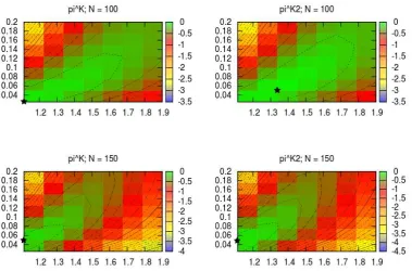
2.1 Simulated log-likelihood surfaces for Kingman-like Beta-coalescents . 42 2.2 Simulated likelihood surface for joint inference of the Beta-coalescent
and mutation rate . . . 43 2.3 Simulated log-likelihood surfaces for challenging Beta-coalescents . . 44 2.4 PAC log-likelihood surfaces for univariate inference . . . 50 2.5 PAC log-likelihood surfaces for joint inference of the Beta-coalescent
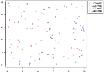
and mutation rate . . . 51 2.6 Sampling locations and observed types of a simulated observation
from a spatial Λ-coalescent . . . 58 2.7 Simulated likelihood surfaces for the spatial Λ-coalescent . . . 59 2.8 Simulated containment probabilities of the hyperbolic diffusion . . . 62 2.9 Simulated hitting probabilities of an ATM network . . . 65 2.10 Simulated likelihood surface for the location of the initial infected
based on an observed SIS epidemic on a network . . . 68 3.1 Limiting posterior probabilities as functions of the observed allele
frequency in the parent-independent, two-allele model . . . 89 3.2 Trace plot of the pseudo-marginal algorithm, the noisy algorithm,
and corresponding delayed acceptance algorithms, targeting the first moment of the Λ-measure . . . 107 3.3 Long run trace plot of the delayed acceptance exact pseudo-marginal
Acknowledgments
Declarations
This thesis is submitted to the University of Warwick in support of my application for the degree of Doctor of Philosophy. It has been composed by myself and has not been submitted in any previous application for any degree.
The work presented (including data generated and data analysis) was carried out by the author.
Parts of this thesis have been published by the author:
• [Koskela et al., 2015a]
• [Koskela et al., 2015b]
• [Koskela et al., 2015c]
Abstract
This thesis has two related aims: establishing tractable conditions for poste-rior consistency of statistical inference from non-IID data with an intractable likeli-hood, and developing Monte Carlo methodology for conducting such inference. Two prominent classes of models, jump diffusions and generalised coalescent processes, are considered throughout. Both are motivated by population genetics applications. Posterior consistency of nonparametric inference is established for joint in-ference of drift and compound Poisson jump components of unit volatility jump dif-fusions in arbitrary dimension under an identifiability assumption. This assumption is straightforward to verify in the diffusion case, but difficult to check in general for jump diffusions. A similar consistency result is established under somewhat weaker conditions for Λ-coalescent processes whenever time series data is available. I also show that Λ-coalescent inference cannot be consistent if observations are contempo-raneous, in stark contrast to the more classical case of the Kingman coalescent.
Abbreviations
• ABC: approximate Bayesian computation
• ATM: asynchronous transfer mode
• CPU: central processing unit
• CSD: conditional sampling distribution
• DNA: deoxyribonucleic acid
• ESS: effective sample size
• GPU: graphical processing unit
• IID: independent and identically distributed
• LHS: left hand side
• MCMC: Markov chain Monte Carlo
• MRCA: most recent common ancestor
• PAC: product of approximate conditionals
• RHS: right hand side
• SDE: stochastic differential equation
• SIS: susceptible-infected-susceptible
Chapter 1
Introduction
Analysis of the likelihood function has been central to statistics for a century [Fisher, 1912, 1922] due to the fact that it (along with the prior in the Bayesian setting) en-codes all of the signal contained in a data set about the data-generating mechanism. Hence analysis of the likelihood yields point estimators of parameter values, confi-dence or credible sets as well as estimators of any other quantity of interest, along with quantitative information about the accuracy of estimates, at least in principle. Let {Pθ, θ ∈ Θ} be a parametric family of statistical models, and x1:n =
(x1, . . . , xn) denote an observed data set. The likelihood function is the joint
prob-ability
L(θ;x1:n) =Pθ(X1 =x1, . . . , Xn=xn),
which is not a tractable function in general. When the observations are independent, the likelihood decomposes into the substantially more tractable product form:
L(θ;x1:n) = n
Y
i=1
Pθ(Xi =xi).
However, there are a myriad of statistical applications in which the independence assumption is either restrictive, or outright false. Asymptotically, the assumption of independence can be relaxed to the much more permissive regularity conditions of local asymptotic normality [Le Cam, 1953, 1956, 1960], under which correlated observations can be treated as arising from a joint Gaussian distribution. Thus it is only necessary to estimate the mean vector and covariance matrix under the Gaussian assumption.
an asymptotic analysis, there is no reason to expect the likelihood function to be tractable. Intractable likelihood functions also arise in e.g. statistical mechanics, inference from diffusions and missing data problems, all of which have a wide range of applications.
The tractability of the likelihood function is important for (at least) two reasons:
1. Maximising the likelihood function is a concrete way of obtaining maximum likelihood estimators,θb, for parameters,θ.
2. Analysis of the likelihood function is central to proving desirable properties of these estimators, such as consistency, unbiasedness, efficiency etc.
In recent decades the desire to carry out these two procedures for increasingly com-plex models and data sets have motivated the development of statistical methods which circumvent the need for an exact likelihood function. An incomplete list of examples addressing point 1. includes the celebrated Metropolis-Hastings algorithm [Metropolis et al., 1953; Hastings, 1970], which only requires likelihood evaluations up to a normalising constant; the sequential Monte Carlo [Doucet and Johansen, 2011] and sequential Monte Carlo sampler [Del Moral et al., 2006] algorithms, which are well suited to missing data problems, rare event simulation and filtering; and exact simulation algorithms for inference from partially observed diffusions with intractable transition probabilities [Beskos et al., 2006, 2009].
A minimal requirement for good statistical inference is that the estimatorθb
isconsistent, i.e. thatθb→θ asn→ ∞, in some appropriate sense. Intuitively, the
notion of consistency corresponds to it being possible to learn the truth from data. In the Bayesian setting consistency can be expressed as the posterior distribution,
P(θ|x1:n)∝Q(θ)Pθ(x1:n), concentrating on a neighbourhood of the parameter which
generates the data, whereQ(θ) is the prior. Standard conditions to ensure posterior consistency are formulated in terms of Kullback-Leibler divergences and exponen-tially consistent hypothesis tests [Schwartz, 1965], which are difficult to verify when the likelihood is intractable. Moreover, many of the natural parameter sets of pro-cesses with intractable likelihood are infinite dimensional — consider for example function-valued coefficients of SDEs — and in thisnonparametric setting posterior consistency is a very delicate property [Diaconis and Freedman, 1986].
The aim of this thesis is twofold:
2. to derive optimised, unbiased sequential Monte Carlo inference algorithms for intractable inference problems.
Both aims are motivated by inference problems in population genetics, where non-parametric inference arises naturally e.g. for the so-called Λ-coalescent family [Pit-man, 1999; Sagitov, 1999] and where both Markov chain Monte Carlo [Kuhner et al., 1995; Wilson and Balding, 1998; Felsenstein et al., 1999; Drummond et al., 2002] and sequential Monte Carlo [Griffiths and Tavar´e, 1994a,b,c; Stephens and Don-nelly, 2000] have a well established role. Despite the motivating application, both results will be presented in some considerable generality: nonparametric consistency for discretely observed jump diffusions as well as Λ-coalescents, and the sequential Monte Carlo algorithms for generic, stopped Markov chains, of which coalescent models are an example. The derivation of the sequential Monte Carlo algorithms will yield very efficient but biased pseudo-likelihood algorithms as a byproduct, and these will also be investigated briefly. Sequential Monte Carlo will be the subject of Chapter 2, while Bayesian nonparametric consistency is developed in Chapter 3.
The key to the sequential Monte Carlo algorithms developed in this thesis will be the notion of time reversal: simulating trajectories of Markov chains in re-verse time. This makes it easy to condition the trajectories to hit sets of small, or even zero probability, which makes the methods well suited for rare event simula-tion. Time reversal is at the core of sequential Monte Carlo inference in population genetics, and the idea of viewing the optimal sequential Monte Carlo algorithm as the time-reversal of the coalescent process has appeared before in [Birkner et al., 2011], but the results of this thesis make the connection transparent enough to be easily generalisable.
1.1
Coalescent processes
Coalescent processes have been a central tool in population genetic modelling and inference ever since their introduction by Kingman [1982a,b]. Kingman’s coa-lescent is a model of the ancestry of lineages sampled from an infinite, panmictic population undergoing random mating. Ancestral trees are generated by merging each pair of lineages into a common ancestor at rate 1, thus reducing the number of lineages by one. The process terminates once the most recent common ances-tor (MRCA) of all sampled lineages is reached, so that a realisation of Kingman’s coalescent is a random, binary tree.
Kingman’s coalescent is the attractor of a broad class of individual-based, finite population models of evolution. This is the class is conveniently described in terms of Cannings models [Cannings, 1974, 1975]. Consider a stationary population of fixed sizen∈N, undergoing random mating in discrete time with non-overlapping generations. At time t ∈ N individual i ∈ {1, . . . , n} =: [n] produces a random number ni(t) of offspring, so that the generation at time t+ 1 is given by the
random vector (n1(t), . . . , nn(t)) withPni=1ni(t) =n. The population is stationary,
and offspring numbers between different generations are assumed independent, so that the vectors {n1(t), . . . , nn(t)}t∈N are IID. Further, assume that each vector is
exchangeable, so that for any permutationσ ∈Sn of [n] it holds that
(n1(t), . . . , nn(t))= (d nσ(1)(t), . . . , nσ(n)(t)),
where= indicates equality in distribution.d
Kingman’s coalescent is obtained by defining the time scale
cn:= E
[n1(1)(n1(1)−1)]
n−1 and thus the rescaled process
(˜n1(t), . . . ,n˜n(t)) := (n1(bt/cnc), . . . nn(bt/cnc)). (1.1)
Ifcn→0 and
E[n1(1)(n1(1)−1)(n1(1)−2)]
cnn2
→0 (1.2)
The assumptions of discrete time and non-overlapping generations have been made for ease of exposition. Neither assumption is necessary for obtaining conver-gence, although the time scalecn may have to be altered when they don’t hold. The
assumption of a fixed population size can also be relaxed. For a detailed exposition on Kingman’s coalescent and coalescent theory, the interested reader is directed to [Wakeley, 2009] and references therein. In particular, the effect of changing popula-tion size, crossover recombinapopula-tion [Griffiths and Marjoram, 1997], natural selecpopula-tion [Krone and Neuhauser, 1997] and spatial structure [Herbots, 1997] on ancestries can all be incorporated into the coalescent framework.
The domain of attraction of Kingman’s coalescent is determined by two cru-cial assumptions: exchangeability of the offspring vectors and the moment conditions
cn→0 and (1.2). The former has a biological interpretation as a neutral,
homoge-neous population with no natural selection or population structure, and the latter as small family sizes compared to the size of the whole population. I will focus on two relaxations of these conditions: allowing high fecundity events in which a small number of ancestors give rise to a significant fraction of the whole population in a small number of generations, and spatial structure across a continuous geography. The resulting families of coalescent models under study are, respectively, the Λ- and Ξ-coalescents for high fecundity events, and spatial Λ-coalescents for geographical structure. As with Kingman’s coalescent, changing population size, recombination [Birkner et al., 2012; Etheridge and V´eber, 2012] and selection [Etheridge et al., 2010, 2014] can be incorporated into both families of coalescents, and a spatially structured version of the Λ-coalescent has also been derived [Heuer and Sturm, 2013]. However, none of these extensions are within the scope of this thesis.
1.1.1 Λ- and Ξ-coalescents
The Λ-coalescents, introduced by Donnelly and Kurtz [1999], Pitman [1999] and Sagitov [1999], generalise Kingman’s coalescent by permitting multiple lineages to merge in one event. Such multiple mergers correspond to high fecundity reproduc-tion events, in which a single individual becomes ancestral to a significant fracreproduc-tion of the whole population in a single generation. The merger rate of any k out of n
lineages is given by
λn,k:=
Z 1
0
rk−2(1−r)n−kΛ(dr)
Cannings-like models withcn→0,
n cnP
(n1(1)> nx)→
Z 1
x
r−2Λ(dr) (1.3)
for 0< x <1, and
E[n1(1)(n1(1)−1)n2(1)(n2(1)−1)]
cnn2
→0 (1.4)
asn→ ∞[M¨ohle and Sagitov, 2001]. Note that while (1.3) permits large family sizes and hence mergers involving more than two lineages with positive probability, (1.4) ensures only one merger can take place at any given time. Simultaneous mergers are ruled out.
Popular choices of Λ include Λ =δ0, which corresponds to Kingman’s
coa-lescent, Λ =δ1 leading to star-shaped genealogies, Λ = 2+2ψ2δ0+ ψ
2
2+ψ2δψ whereψ∈
(0,1] [Eldon and Wakeley, 2006], Λ = Beta(2−α, α) whereα ∈(1,2) [Schweinsberg, 2003; Birkner and Blath, 2008; Birkner et al., 2011], and Λ(dr) =cδ0(dr) +1−2crdr
wherec∈[0,1] [Durrett and Schweinsberg, 2005]. Birkner and Blath [2009] provide a review of Λ-coalescents.
The Λ-coalescents allow multiple mergers, but only permit one merger at a time. They are generalised further by the Ξ-coalescents, which permit any number of simultaneous, multiple mergers. Ξ-coalescents were introduced by Schweinsberg [2000] and M¨ohle and Sagitov [2001], and can be expressed in terms of a finite measure Ξ on the infinite simplex
∆ =
(
r= (r1, r2, . . .)∈[0,1]N: ∞ X
i=1
ri ≤1
)
.
Again, Ξ can be taken to be a probability measure without loss of generality. Letλn;k1,...,kp;s denote the rate of jumps involving p ≥1 mergers with sizes
k1, . . . , kp, with s=n−Ppi=1ki lineages not participating in any merger. The total
number of lineages before the mergers is denoted byn. This rate is given as
λn;k1,...,kp;s:=
Z
∆ s
X
l=0
s l
X
i1∈N
. . . X
ip+l∈N
rk1
i1 . . . r
kp
iprip+1. . . rip+l
(1−P∞i=1ri)s−l
P∞
i=1r2i
Ξ(dr).
Note that if Ξ assigns full mass to the set{r∈∆ :r2 =r3=. . .= 0}, the resulting
Ξ-coalescents correspond to Cannings-type models for which limn→∞cn= 0
and the limits
lim
n→∞
E(n1(1))k1. . .(np(1))kp
cnnk1+...+kp−p
(1.5) exist for any p ∈ N and k1, . . . , kp ∈ N, where (n)k := n(n−1). . .(n−k+ 1)
is the falling factorial. Any combination of p simultaneous mergers involving, re-spectively,k1, k2, . . . , kp lineages is permitted with positive probability provided the
corresponding limit (1.5) is positive. The case limn→∞cn=c >0 results in discrete
time versions of Ξ-coalescents [M¨ohle and Sagitov, 2001].
1.1.2 Spatial Λ-coalescents
This section presents the spatial Λ-coalescent, introduced by Etheridge [2008] and Barton et al. [2010a] as a generalisation of Kingman’s coalescent for structured pop-ulations in a continuous geography. Previous generalisations typically incorporate spatial structure by modelling the geography as a graph with panmictic populations at the vertices and migration along edges [Wright, 1931; Kimura, 1953]. Natural population habitats are continuous, which makes an accurate subdivision difficult to specify. The choice of graph structure can also have an effect on inference. An-other alternative is the Isolation by Distance model [Wright, 1943; Mal´ecot, 1948], which suffers from the “Pain in the Torus” [Felsenstein, 1975] of either extinction or unstable population growth and clustering. The “Pain in the Torus” can be avoided by local population density regulation which stabilises the population, but typically renders models intractable.
The spatial Λ-coalescent circumvents both these difficulties by being defined on a continuous geography, and achieving local density regulation tractably by mod-elling reproduction via extinction-recolonisation events driven by a space-time Pois-son process, which is independent of the state of the population. For concreteness I focus on a two-dimensional geography, which I take to be a torus of side length
L >0 denoted by T := T(L). Let z1:n := (z1, . . . , zn) ∈ T(L)n be the locations of
n∈N sampled lineages. For simplicity I assume all locations are distinct.
The dynamics of the spatial Λ-coalescent are driven by a Poisson processN
on R×T with ratedt⊗dx. The points (t, x) ∈N model extinction-recolonisation
events, with the two co-ordinates specifying the time and place of the event re-spectively. Tracing backwards in time, at each point (t, x) ∈N, all lineages within
Br(x), a closed ball of radiusr >0 centred atx, flip a coin with success probability
the event. Once the whole sample has merged into a single lineage (the MRCA), the process terminates yielding a random tree with nodes labelled by geographical locations and edges denoting jumps in spatial locations and mergers.
This is the so called disc model of the spatial Λ-coalescent process defined by the replacement kernelu1Br(x)(y), but it is straightforward to construct variants
by using e.g. Gaussian or heavy-tailed replacement around each event centrex. The Gaussian replacement model has been studied in [Barton et al., 2010b], and the heavy-tailed case in [Berestycki et al., 2013].
The spatial Λ-coalescent is also the attractor of high density limits of a broad class of individual-based models. Examples of such families are described in [Etheridge and Kurtz, 2014]. Barton et al. [2013b] provide a review of spatial Λ-coalescents and related processes.
1.1.3 Mutation
In addition to describing ancestral relationships between lineages, coalescent pro-cesses can be used to tractably sample genetic types from populations. In the notation of Paul and Song [2010], suppose that the genetic material of an organism of interest is formed of k linearly arranged loci, or a haplotype. Suppose the state of a locusl ∈ [k] can be one of a finite collection of alleles El = {1, . . . ,|El|}, and
mutates at rate θl with mutant alleles sampled from a stochastic matrix M(l). Let
θ := P
l∈[k]θl denote the total mutation rate, H := E1×. . .×Ek denote the set
of possible haplotypes, and let M denote the stochastic matrix on H formed as a mixture distribution from weights {θl/θ}l∈[k] and mixture components {M(l)}l∈[k].
Assume also thatM has a unique stationary distributionm. For a haplotypeh∈ H
leth[l] denote the allele at locuslof haplotypeh, and letSla(h) denote the haplotype obtained from hby substituting allele aat locus l.
Whenθ >0 andM is irreducible, all haplotypes will persist in the population and mutation is called recurrent. Given a realised coalescent tree, haplotypes from a stationary population can be generated by sampling a haplotype for the MRCA from m, and propagating it along the edges of the tree with mutations occurring at rate θand mutant haplotypes sampled from M. Non-stationary samples can be obtained by changing the distribution of the MRCA haplotype, but I will focus on the stationary case in this thesis.
When incorporating mutation, the coalescent processes introduced above can be viewed as stochastic processes Π := (Πt)t≥0 taking values in PnH, the set of H
coalescent starts from the unlabelled, trivial partition ψn := {{1},{2}, . . . ,{n}},
mergers of lineages correspond to merging the corresponding blocks in the partition, and haplotype labels can be propagated along the realised tree as described above once the MRCA is reached. Of course, in the spatial case it is also necessary to label the partitions with their spatial locations while the lineages are coalescing, and the resulting tree will be labelled both with haplotypes and locations.
As with the coalescent processes, I will denote the resulting laws on spaces of labelled trees by PΛn(·), PnΞ(·) and PSLn (·) for Λ-, Ξ- and spatial Λ-coalescents respectively. The corresponding expectations will be denoted by EnΛ[·], EnΞ[·] and
EzSL1:n[·], where in the spatial Λ-coalescent case the vectorz1:ndenotes initial sampling
locations. The symbolsPn(·) and En[·] will refer to generic coalescent processes.
The finite alleles model is arguably the most realistic model of mutation, as it mimics the structure of DNA sequences whenEl ={A, C, G, T}for each l∈[k].
However, it can result in very computationally intensive simulations and inference when the number of loci is large. I will focus on recurrent finite alleles mutation in this thesis, but conclude the section by mentioning some popular alternatives.
The infinite alleles model depicts the allele at each locus as a point along the unit interval. Mutations occur at rate θ, and result in sampling a new allele uniformly, so that all information of the parental allele is lost. This model is coarse, but was often appropriate before modern DNA sequencing became widespread, when it was only possible to determine whether or not two DNA segments were identical. The infinite sites model is a refinement of the infinite alleles model, in which haplotypes are depicted as a continuous line segment. Mutations occur at rate θ, and result in a mutant allele at a uniformly sampled location along the haplotype. Sampled haplotypes are identified relative to a reference, usually the ancestral hap-lotype, and their state can be specified by listing all the mutant locations at which the reference and sample differ. Note that no location can ever mutate more than once, which is problematic because real genetic data sets frequently contain loci with three or more observed alleles. However, the infinite sites assumption can be reasonable when the number of sampled loci is large, and the model is computation-ally more tractable than the finite alleles model. Note also that the infinite alleles model can be obtained from the infinite sites model by simply recording whether or not at least one mutation has taken place along a sampled haplotype.
microsatellites, which consist of repeating a fixed pattern of DNA, e.g. AT, a variable number of times, so that the state of a microsatellite locus might be (AT)m for any
m∈Z, again relative to a reference number of repeats.
1.2
Jump diffusions and duality
A successful model in population genetics consists of a historical model of ancestry, as well as a corresponding model of population allele frequencies forwards in time. When endowed with a set of haplotypes H and inheritance of haplotypes from parents, the Cannings models and their generalisations introduced in Section 1.1 are examples of finite population models of allele frequencies. Infinite population limits are most naturally expressed in terms of measure-valued jump diffusions. In this section I will introduce the Viot, Ξ-Fleming-Viot and spatial Λ-Fleming-Viot processes, corresponding in the obvious way to the coalescent processes outlined in Section 1.1. I will also make the correspondence precise via a duality relation which connects each measure-valued allele frequency process to its corresponding coalescent.
1.2.1 Λ- and Ξ-Fleming-Viot processes
Let ∆H := {x ∈ [0,1]|H| : Pdi=1xi = 1} denote the |H|-dimensional probability
simplex. The Λ-Fleming-Viot processXΛ:= (XΛt)t≥0 with mutation rates{θl}l∈[L],
mutation matrix M and Λ-measure Λ ∈ M1([0,1]) is a ∆H-valued jump diffusion
with generator
GΛf(x) =Λ({0}) 2
X
i,j∈H
xi(δij −xj)
∂2 ∂xi∂xj
f(x) +θ X
i,j∈H
xj(Mji−δij)
∂ ∂xi
f(x)
+X
i∈H
xi
Z
(0,1]
[f((1−r)x+rei)−f(x)]r−2Λ(dr) (1.6)
acting on functionsf ∈C2(∆H), whereei is the canonical unit vector with a 1 in the
diffusion (see e.g. [Durrett, 2008], chapters 7 and 8) on ∆Hwith recurrent mutation.
The law of a Λ-Fleming-Viot process with initial condition x ∈ ∆H will
be denoted by PΛx(·), and expectation with respect to this law by EΛx[·]. I will
suppress dependence on initial conditions whenever the stationary process is meant. For bounded f : ∆H 7→ R, let PtΛf(x) := EΛx[f(XΛt)] be the associated transition
semigroup, pΛt(x,y)dy :=PΛx(XΛt ∈dy) be the transition density andπΛ(x)dx the
corresponding unique stationary density on ∆H. The transition semigroup is Feller
for any Λ∈ M1([0,1]) [Bertoin and Le Gall, 2003], and all densities are assumed to
exist with respect to a common dominating measuredx.
The following duality between Λ-coalescents and Λ-Fleming-Viot jump dif-fusions was established in Bertoin and Le Gall [2003]:
EΛ
"
Y
h∈H
XΛt(h)nh
#
=EnΛ
"
Y
h∈H
m(h)|ΠΛt(h)|
#
, (1.7)
wherenh denotes the number of observed individuals of haplotype h∈ H sampled
IID from the random measure XΛt, and |ΠΛt(h)| denotes the number of blocks in partition ΠΛt of haplotype h ∈ H. In words, it states that the distribution of the allele frequencies generated by a Λ-coalescent started from ψn coincides with the
distribution of a multinomial sample drawn from the corresponding stationary Λ-Fleming-Viot process.
Birkner et al. [2009] constructed the Ξ-Fleming-Viot process, and established the same duality between it and the Ξ-coalescent. The Ξ-Fleming-Viot process is a jump diffusion similar to the Λ-Fleming-Viot process, but with a wider class of possible jumps reflecting the more general mergers of the Ξ-coalescent. I denote the Ξ-Fleming-Viot process byXΞ := (XΞt)t≥0.
With state space as above, the Ξ-Fleming-Viot process is the jump diffusion with generator
GΞf(x) = Ξ({0}) 2
X
i,j∈H
xi(δij−xj)
∂2 ∂xi∂xj
f(x) +θ X
i,j∈H
xj(Mji−δij)
∂ ∂xi
f(x)
Z
∆ Z
HN
"
f 1− krk1x+
∞ X
i=1
rieh0i
!
−f(x)
# X
h∈H
xhδh
!⊗N
(dh0)Ξ(dr)
krk2 2
,
where Ξ is a probability measure on the infinite simplex
∆ :=
(
r∈[0,1]N:
∞ X
i=1
ri = 1
)
and krkp denotes thep-norm of r. For more details, including the specification of a suitable class of test functions, see Proposition 1.3 of [Birkner et al., 2009]. The law, expectation, transition semigroup, density and stationary distribution of the Ξ-Fleming-Viot process will be denoted byPΞx(·),ExΞ[·], PtΞ,pΞt(x,y)dyand πΞ(x)dx,
respectively.
1.2.2 Spatial Λ-Fleming-Viot processes
The spatial Λ-Fleming-Viot process is the analogue of the Λ-Fleming-Viot process, and describes the allele frequencies at each point in the continuous geography. It was introduced by Barton et al. [2010a], who also established a duality between the spatial Λ-Fleming-Viot process and the spatial Λ-coalescent.
Recall the Poisson process N from Section 1.1.2. The spatial Λ-Fleming-Viot process XSL := (XSL
t (x,·))x∈T,t≥0 specifies a probability measure on ∆H at
each location x ∈ T and time t ≥0. This probability measure describes the allele frequencies in the population at that location and time.
The dynamics of XSL are driven by N, in that at each point (t, x) ∈ N a
parental location z is sampled uniformly from Br(x), and a parental haplotype h
fromXSL(t, z,·). The surfaceXSL then undergoes the update
XSLt (y,·) =
(1−u)XSLt−(y,·) +uδh(·) ify∈Br(x) XSLt−(y,·) otherwise.
The spatial analogue of the duality relation (1.7) has precisely the same interpretation as before: the distribution of a sample drawn at locationsz1:nfrom a
stationary Λ-Fleming-Viot process coincides with that obtained by running a spatial Λ-coalescent from those locations until merging to the MRCA, sampling an ancestral type frommand propagating types along the coalescent tree with mutations at rate
θsampled from M.
The duality relation (1.7), and its generalisations will play a central role in designing sequential Monte Carlo inference algorithms for evaluating likelihoods of multinomial samples from the allele frequency processes. They will also prove convenient in proving the nonparametric consistency results of Section 3.3.1.
1.2.3 General jump diffusions
section introduces the general formulation of a time homogeneous jump diffusion on a domain Ω⊆Rd in preparation for stating these results.
Jump diffusions are a broad wide class of stochastic processes encompassing systems undergoing deterministic mean-field dynamics, microscopic diffusion and macroscopic jumps. Jump diffusions are used as models across broad spectrum of applications, such as economics and finance [Merton, 1976; Aase and Guttorp, 1987; Bardhan and Chao, 1993; Chen and Filipovi´c, 2005; Filipovi´c et al., 2007], biology [Kallianpur, 1992; Kallianpur and Xiong, 1994; Bertoin and Le Gall, 2003; Birkner et al., 2009] and engineering [Au et al., 1982; Bodo et al., 1987]. They also contain many important families of stochastic processes as special cases, including diffusions and L´evy processes.
A general time-homogeneous, d-dimensional jump diffusion X := (Xt)t≥0 is
the solution of a stochastic differential equation of the form
dXt=b(Xt)dt+σ(Xt)dWt+c(Xt−, dZt) (1.8)
X0 =x0
where σ : Ω 7→ Rd×d is known as the diffusion coefficient, b : Ω 7→
Rd as the drift
and c : Ω×Rd 7→
Rd0 as the jump coefficient. The process W := (Wt)t≥0 is a
d-dimensional Brownian motion andZ:= (Zt)t≥0 is a pure jump L´evy process with
jumps in Rd0 :=Rd\ {0}. The processZis taken to be independent of W, and has
L´evy measure M(dz) satisfying
Z
Rd0
(kc(x,z)k22∧1)M(dz)<∞
for anyx∈Rd. Note that the space in whichZtakes values can also be a more
gen-eral Lusin space [El Karoui and Lepeltier, 1977], but this possibility is not considered in this thesis for ease of notation.
Under regularity conditions summarised below, jump diffusions are recurrent, ergodic Feller-Markov processes with transition densities pt(x,y)dy and a unique
be well defined are non-singularity ofσ and the following symmetry condition [Yu, 2007; A¨ıt-Sahalia, 2008]:
∂(σ−1)ij(x)
∂xk
= ∂(σ
−1) ik(x)
∂xj
for all i, j, k ∈ {1, . . . , d}.
Whenever well defined, this transformation maps a diffusion with generalσ to one with unit diffusion but altered drift and jump size distribution. Results which can be deduced for the transformed diffusion must then be mapped by via an inverse Lamperti transform to the original problem.
Proposition 1. Assume thatc(·,0)≡0, and that there exist constantsC1, C2, C3, C4 >
0 such that
kb(x)−b(y)k22+
Z
Rd0
kc(x,z)−c(y,z)k22M(dz)≤C1kx−yk22 (1.9)
kc(x,z)−c(x,ξ)k22≤C2kz−ξk22 (1.10)
For every x∈Ω :kxk2> C3 the following holds: x·b(x)≤ −C4kxk22 (1.11) Z
Rd0:kzk2>1
kzk22M(dz)<∞. (1.12)
Then(1.8)has a unique, ergodic weak solutionXwith the Feller and Markov proper-ties. Furthermore,X has a unique stationary density πb,ν(x)dx with a finite second moment, and the associated semigroup Ptb,ν has transition densities pb,νt (x,y)dy. Proof. Existence and uniqueness of X are obtained from (1.9), as well as the lin-ear growth bounds implied by Lipschitz continuity, by Theorem 6.2.9 of [Apple-baum, 2004]. Theorem 6.4.6 of [Applebaum, 2004] gives the Markov property under the same conditions. Finally, the corollary in Appendix 1 of [Kolokoltsov, 2004] yields the Feller property. In turn, the Feller property and the fact that log(1 +kξk2)−1kξk22 → ∞ as kξk2 → ∞ mean that the hypotheses of Theorem
1.1 of [Schilling and Wang, 2013] are fulfilled, so that X has bounded transition densities with respect to the Lebesgue measure.
Existence and uniqueness ofπb,ν, as well as ergodicity ofX will follow from Theorem 2.1 of [Masuda, 2007], the hypotheses of which will now be verified. Along withc(·,0)≡0, conditions (1.9) and (1.10) above imply Assumption 1 of [Masuda, 2007]. Now, for everyu∈(0,1) let
bu(x) :=b(x)−
Z
u<kzk1≤1
Assumption 2(a)’ of [Masuda, 2009] requiresX to admit bounded transition densi-ties, and the diffusion which solves
dXut =bu(Xut)dt+σ(Xut)dWt
to be irreducible for each u > 0. Boundedness of the transition density of X was established above, and irreducibility ofXu holds because σ ≡1 by Theorem 2.3 of [Stramer and Tweedie, 1997].
Next, I will verify Assumptions 3 and 3* of [Masuda, 2007] by checking the conditions of Lemma 2.4’ of [Masuda, 2009]. The diffusion coefficient is constant, and hence o(kxk21−q/2) for any q ∈ (0,2). Condition (1.12) is the corresponding hypothesis of [Masuda, 2009], and bothkxkq2−2x·b(x) → −∞and kxk−22x·b(x)≤ −C4 follow from (1.11). Hence, Assumptions 3 and 3* of [Masuda, 2007] hold.
This yields ergodicity (and mixing) by Theorem 2.1 of [Masuda, 2007], and second moments of the stationary distribution (and exponential mixing) by Theorem 2.2 of [Masuda, 2007].
It remains to show the invariant measure has a density. By combining Propo-sition 5.1.9 and Theorem 5.1.8 of [Fornaro, 2004] it can be seen that invariant mea-sures of irreducible strong Feller processes are equivalent to the associated transition probabilities, which is sufficient in this case. Assumption 1 of [Masuda, 2007] and Assumption 2(a)’ of [Masuda, 2009] imply irreducibility ofX (c.f. Claim 1 on page 42 of [Masuda, 2007]). Condition (1.9) guarantees the strong Feller property by The-orem 2.3 of [Wang, 2010]. Hence the invariant measure has a density with respect to the transition densities, and thus also the Lebesgue measure. This concludes the proof.
1.3
Sequential Monte Carlo
Liu [2001]; Del Moral [2004]; Fearnhead [2008]; Doucet and Johansen [2011], and references therein).
Sequential importance sampling consists of sampling from a sequence of pro-posal distributions to build up a single, high-dimensional realisation. The propro-posals are typically not the conditional distributions of the model of interest, and so sam-ples must be reweighted by the Radon-Nikodym derivative of the model and the proposal. LetX1:n:= (X1, . . . , Xn) be a random vector with lawP, and suppose it
is of interest to evaluate an intractable functional
E[f(X1:n)] =
Z
f(x1:n)P(dx1:n)
=
Z
. . .
Z
f(x1:n) n
O
i=1
P(dxi|X1:i−1=x1:i−1), (1.13)
with the convention that x1:0 = 0. This expectation can be approximated by the
sample mean of function evaluations of f on data {x(1:i)n}k
i=1 with x
(j)
i:n IID
∼ P, but this approach can lead to very high variance if the dominant contributions to the integral are from regions which are unlikely underP. Variance can be reduced by introducing a proposal distributionQwithP Q, and estimating (1.13) with
b
I := 1
k
k
X
j=1
f(x(1:jn))
n
O
i=1
P(dx(ij)|X1:(ji)−1 =x(1:ji)−1)
Q(dx(ij)|X1:(ji)−1 =x(1:j)i−1) =: 1
k
k
X
j=1
f(x(1:jn))wn(x(1:jn)),
withx(1:jn) IID∼ Q.
Sequential Monte Carlo involves the combination of sequential importance sampling with a resampling step, where particles{x(1:j)n}k
j=1and weights{w(x
(j)
1:n)}kj=1
are built up in parallel. The weighted collection can then be resampled at interme-diary steps to discard particles with low weight and duplicate promising ones with high weight. Good choices of Q and resampling schedule can dramatically reduce the variance of estimators, and can be shown to be asymptotically efficient under mild conditions [C´erou et al., 2011]. On the other hand, poor choices ofQcan yield estimators with higher variance than na¨ıve Monte Carlo [Glasserman and Wang, 1997].
Good design of a resampling schedule is also crucial, as without resampling the variance of estimators typically increases exponentially in the number of sequen-tial steps [Doucet et al., 2001; Liu, 2001]. In the simplest case particles are resampled multinomially between theith and (i+ 1)th sequential step with probabilities pro-portional to their respective importance weights{w(x(1:ji))}k
equalised, subject to preserving the total weights of the particle ensemble, and the resulting collection of particles is treated as the starting point of generating the (i+ 1)th sample. While intuitive, multinomial resampling is outperformed in terms
of variance by other, more complicated resampling mechanisms [Douc et al., 2005]. It is also typically detrimental to resample at every stage of the algorithm. The most common heuristics for when resampling should be performed are based on the effective sample size (ESS) of the ensemble falling below a specified threshold [Kong et al., 1994].
1.3.1 SMC for coalescent processes
It is of great interest to estimate parameters describing the evolutionary history of a population from a sample of DNA sequences. This can be done by assuming an appropriate coalescent model, writing down a likelihood as a function of the parameters and evaluating the likelihood for various parameter values. Such an approach is common to both frequentist and Bayesian analyses, with the additional stage of prescribing a prior distribution on parameters in the Bayesian case.
Let n ∈ N|H| denote an observed configuration of allele frequencies of size
n:=P
h∈Hnh, andθ∈Θ be a parameter value and a parameter space, respectively.
Let A ∈ A denote, respectively, a realisation of the coalescent ancestry and the space of possible ancestries, i.e. the support of Pn. For A ∈ A define pn(A) = 1
if the haplotypes at the leaves of A gives rise to allele frequencies n, and pn(A) =
0 otherwise. The likelihood L(θ;n) can be decomposed by conditioning on the ancestry as
L(θ;n) =En[1n(A)|θ] =
Z
A
pn(A)Pn(A|θ)dA (1.14)
The likelihood function L will be endowed with a superscript Λ, Ξ or SL when a particular coalescent model is meant.
The space of coalescent trees is prohibitively large for all but trivially small data sets, so in practice the integral on the RHS of (1.14) is approximated by Monte Carlo, or replaced by a pseudo-likelihood from a simpler model. A na¨ıve Monte Carlo approximation is obtained by simulating IID ancestries A1, . . . , Ap from Pn, and
computation, and pseudo-likelihood methods, which will be outlined in the next section. Developing good approximations to (1.14) for large, whole-genome data sets under any but the simplest genetic models remains an open problem.
SMC has a well established role in population genetic inference as a means of approximating likelihoods. In this context the method was introduced by Grif-fiths and Tavar´e [1994a,b,c, 1999], who derived a recursion for quantities of interest under Kingman’s coalescent [Kingman, 1982a,b] and simulated a Markov chain to approximate its solution. Their approach was identified as importance sampling by Felsenstein et al. [1999]. SMC has been investigated and applied to genetic problems such as demographic and other parameter inferences [Griffiths and Marjoram, 1996; Fearnhead and Donnelly, 2001; De Iorio et al., 2005; Griffiths et al., 2008; Gorur and Teh, 2008; Hobolth et al., 2008; Jenkins and Griffiths, 2011].
In brief, the idea of SMC for coalescent processes is to sample the ancestry
A sequentially in reverse time, so that every sample will be compatible with the leaves and promising ancestries can be prioritised in favour of ones which are in-compatible with the dynamics of the coalescent. Let {Ai}Ki=0 denote the state of
the ancestryimutation or coalescence events into the past, so that A0 denotes the
coalescent leaves, AK denotes the haplotype of the MRCA and the other Ai’s are
intermediate configurations along the tree. Let Q be a proposal distribution
sat-isfying supp(Pn) ⊆ supp(Q). Then (1.14) can be decomposed into the sequential
updates
L(θ;n) =
Z
A
m(AK) K−1
Y
i=0
Pn(Ai|Ai+1, θ) Q(Ai+1|Ai, θ) Q
(dAi+1|Ai, θ) (1.15)
Note that the indicator function pn(A) is no longer needed as all trees will be
compatible with the data by construction. Coalescent histories {{A(ij)}Kj i=0}
p j=1 can
now be sampled according to the proposal distribution Q, and the likelihood can
be approximated by the weighted average Lb(θ;n) = p−1
Pp
j=1wKj where wK =
Pn(A|AK,θ)
Q(A|θ) m(AK) is the importance weight associated with the j
th fully
recon-structed coalescent tree.
Choice of proposal distributionQ is crucially important to the efficiency of
the SMC algorithm. The optimal proposal (in terms of estimator variance) is the conditional distribution Pn(A|n), in which case all particle weights equal the true
likelihood by Bayes’ theorem:
Pn(A|AK, θ)m(AK) Pn(A|n, θ) =
Pn(A|θ)Pn(n|θ)
Pn(n|A, θ)Pn(A|θ) =Pn(n|θ),
proba-bility one, and has zero variance.
Unfortunately, the conditional distribution is as intractable as the likelihood. The typical approach of approximating the optimal proposal distribution using large deviations [Sadowsky and Bucklew, 1990] is also rendered intractable by the high dimension of the space of coalescent trees. Progress can be made by designing proposal distributions which mimic the features of the optimal proposal distribu-tion. This was done for Kingman’s coalescent by Stephens and Donnelly [2000], who expressed the optimal sequential proposal distribution in terms of a family of con-ditional sampling distributions (CSDs). The CSDs are also intractable in general, but the authors introduced an approximation which yielded dramatic improvements in efficiency and accuracy in comparison to earlier SMC algorithms. However, even optimised SMC algorithms fail to scale to modern data sets, so that scalable but biased methods have also received much interest.
Approximating the CSDs for various generalisations of Kingman’s coalescent has received plenty of attention, both as a means of deriving approximations to the optimal importance sampling algorithm and due to the product of approximate conditionals (PAC) method introduced by Li and Stephens [2003]. The PAC algo-rithm is an example of the scalable but biased methods mentioned above. De Iorio and Griffiths [2004a,b] derived an approximation to finite alleles CSDs based on the Fleming-Viot generator while Paul and Song [2010] provided a genealogical inter-pretation and included crossover recombination. Further approximations based on hidden Markov models have been obtained by Paul et al. [2011] and Steinr¨ucken et al. [2013b], and applied by Sheehan et al. [2013].
In the context of coalescent processes, resampling should take into account the weight of the particleandthe progress it has made towards the MRCA. This can be achieved by introducing a sequence of intermediate sets; propagating all samples until they hit the next set; and performing resampling based on current weights once all particles have been stopped. This has been alternatively termed multilevel SMC or stopping-time resampling in Section 12.2 of [Del Moral, 2004] and in [Chen et al., 2005] respectively. It is natural to define the sets based on the number of coalescence and mutation events encountered by the partially reconstructed tree. This approach was investigated by Chen et al. [2005] and Jenkins [2012], and found to yield dramatic improvements to the accuracy of SMC algorithms.
1.3.2 Alternatives to SMC
com-putation (ABC) and product of approximate conditionals (PAC). I will present a brief simulation study of the PAC algorithm for Λ-coalescents in Section 2.4, for which this serves as an introduction, and the other two methods are included for completeness. For further details of MCMC and ABC for population genetics, the interested reader is directed to [Marjoram and Tavar´e, 2006], and references therein. MCMC involves constructing a Markov chain onA whose stationary distri-bution is the conditional law of the coalescent given the observed data,Pn(·|n). The
a simulated trajectory of this Markov chain can be used as an autocorrelated sample from Pn(·|n). Provided the chain has been run sufficiently long, the collection of
samples closely approximates a sample from the target posterior distribution. A typical implementation of this idea is the Metropolis-Hastings algorithm [Metropolis et al., 1953; Hastings, 1970], which is based on an arbitrary transition kernelq :A 7→ M1(A). If the current state of the chain isA, a step is generated by
sampling a proposalA0∼q(A,·), and the proposed step is accepted with probability
1∧Pn(A
0|n)q(A0, A)
Pn(A|n)q(A, A0).
The ratio of conditional distributions can be evaluated by Bayes’ theorem, even though the numerator and denominator individually are intractable. If the move is rejected then the chain remains atA. This algorithm can be extended to parameter inference by extending the state space of the chain to the product space A ×Θ, introducing transition kernels on the extended space, and marginalising the resulting sample overA.
Kuhner et al. [1995] and Felsenstein et al. [1999] developed a Metropolis-Hastings algorithm for Kingman’s coalescent in which moves are proposed by sam-pling a node uniformly at random in the coalescent tree, disconnecting it from it’s parent and reattaching it after an exponentially distributed waiting time to a uni-formly sampled parent edge alive at the time of the merger, or the MRCA if it survives past the current MRCA. Other proposal mechanisms have also been in-vestigated for Kingman’s coalescent, and it’s various generalisations [Wilson and Balding, 1998; Nielsen, 2000; Wilson et al., 2003].
Like SMC, MCMC algorithms are unbiased but suffer the high dimension-ality of the space of coalescent trees. Hence faster, heuristic methods have become prominent for modern genetic data sets. ABC and PAC algorithms are two examples of such heuristic methods.
θ ∈ Θ from a prior Q(dθ), and then data n|θ ∼ L(dn|θ) from the model. The proposal is accepted ifn=n∗, wheren∗ denotes the observation. The distribution of the accepted proposals is the posteriorQ(dθ|n).
However, the data is often extremely high-dimensional and hence the prob-ability that n = n∗ is vanishingly small, or 0 when simulated data has a density. The innovation of the ABC algorithm is to introduce a summary statisticS(n) and a toleranceε >0, and accept the proposal whenkS(n)−S(n∗)k< εin some norm. The algorithm is exact ifSis a sufficient statistic andε= 0, but typically neither of these requirements is feasible and the resulting algorithm is approximate. The ba-sic rejection ABC algorithm has been improved upon in numerous ways [Beaumont et al., 2002; Marjoram et al., 2003; Sisson et al., 2007; Beaumont et al., 2009]. The interested reader is directed to [Beaumont, 2010] for a review of ABC algorithms applied to evolutionary and ecological problems.
The PAC algorithm of Li and Stephens [2003] is based on a decomposition of the likelihood into a product of CSDs, and substituting a tractable, heuristic version of the CSDs in place of the intractable, true CSDs. Suppose that observed allele frequencies n are generated by haplotypes h1:n = (h1, . . . , hn) ∈ Hn. Then
the likelihood can be written as
L(θ|n) =Pn(h1:n|θ) =π(hn|h1:n−1, θ)π(hn−1|h1:n−2, θ). . . π(h2|h1, θ)π(h1, θ),
where π(h|h1:n) denotes the distribution of the type of the (n+ 1)th leaf of a
coa-lescent tree, given the types of the firstnleaves.
Approximate CSDs are typically not exchangeable so that the value of the approximation depends on the choice of ordering of haplotypes. This difficulty could be overcome completely by averaging over all possible orderings, but the computational cost is too high for practical data sets. Instead, a common approach is to average over a small, random subset of permutations [Li and Stephens, 2003]. Coalescent processes and their dual diffusions have been instrumental in designing heuristic approximations to CSDs [Fearnhead and Donnelly, 2001; De Iorio and Griffiths, 2004a,b; Paul and Song, 2010; Paul et al., 2011; Sheehan et al., 2013; Steinr¨ucken et al., 2013b], and the resulting PAC algorithms are widely used due to their scalability.
1.4
Bayesian nonparametric inference
As outlined above, Bayesian inference rests on the specification of a prior distribution
beliefs about the parameter set Θ. The nonparametric development is to allow Θ to be infinite dimensional, yielding greater modelling flexibility at the cost of greater analytical and computational challenges. Typical nonparametric model sets include spaces of functions (e.g. Cb2(Ω) for some Ω ⊆ Rd) or measures (e.g. M
1([0,1])). I
will abuse terminology and refer to elements of such spaces as “parameters”, with the understanding that they may be infinite dimensional.
Givenn∈Ndata pointsx1:n, the central object of Bayesian inference is the
posterior distribution, defined for setsA⊂Θ as
Q(A|x1:n) :=
R
APθ(x1:n)Q(dθ)
R
ΘPθ(x1:n)Q(dθ)
. (1.16)
It is well known that in the Bayesian setting the posterior contains all the informa-tion about the parameter carried by the data. In the nonparametric setting neither existence nor uniqueness of the posterior is guaranteed. When a unique posterior does exist, it is given by (1.16). I will neglect issues of existence and uniqueness, and simply assume that a unique posterior exists.
The next consideration is computing the posterior. This can be done ana-lytically for so calledconjugate pairs of priors and likelihoods. Theses are pairs for which the prior and posterior both belong to the same family with altered parame-ters. Examples in the parametric case include beta priors and binomial likelihoods for estimating the binomial success probability, Gaussian priors and likelihoods for estimating the mean, and Gamma priors with Poisson likelihoods for estimating the rate. A nonparametric example is the Dirichlet process prior [Ferguson, 1973] with IID observations for estimating the unknown sampling distribution. Conjugate fam-ilies impose very restrictive assumptions on the prior, and are often not available, most prominently whenever the likelihood is intractable. When conjugate priors are not available or appropriate, the posterior typically has to be approximated numerically, using Monte Carlo or other methods. This setting is the focus of this thesis.
In addition to reflecting prior information, the prior distribution Q can be seen as specifying a model for learning parameters from data. From this perspective, it makes sense to ask that Q(·|x1:n) concentrates on the “true”, data generating
parameterθ0 asnincreases, reflecting the potential to learn the true model from a
sufficient amount of data. This property is known as posterior consistency, which can be stated more formally as
lim
for any ε > 0 and some norm k · k on Θ, for some appropriate norm, topology and mode of convergence. In the nonparametric setting, posterior consistency is an intricate property which depends in subtle ways on Θ and Q. However, it is also regarded as a minimal requirement for well justified Bayesian inference [Diaconis and Freedman, 1986]. The typical properties required of the prior and the parameter space for posterior consistency to hold are a prior mass condition, i.e. Qmust place sufficient mass in a neighbourhood of θ0 (and, in particular, not exclude it), and
regularity conditions to suitably limit the “size” of Θ.
Stronger, and more analytically demanding forms of posterior asymptotics consist of identification of contraction rates for consistent posteriors, and ultimately Bernstein-von Mises theorems:
sup
A∈B(Θ)
|Q(A|x1:n)−µ(ˆθ,Σ)(A)| →0,
whereµis a Gaussian measure on Θ (see Section 6.3 of [Dashti and Stuart, 2016] for an overview of Gaussian measures on infinite dimensional spaces), ˆθ is an efficient estimator of the posterior mean and Σ is the posterior covariance. Contraction rates are typically established by constructing hypothesis tests with exponentially small error probability Schwartz [1965], for example in [Ghosal et al., 2000; Ghosal and van der Vaart, 2007; Gugushvili et al., 2015; Nickl and S¨ohl, 2015] in various nonparametric settings. The main drawback of this approach is the need to be able to construct exponentially consistent tests, which is rarely possible when the likelihood is intractable.
The Bernstein-von Mises theorem bridges the Bayesian and frequentist worlds by enabling the computation of asymptotic, frequentist estimators and confidence regions from the posterior. The earliest proof in a parametric setting was pub-lished by Doob [1949], and the modern form for parametric statistics was developed by Le Cam [1986]. Like contraction rates, nonparametric versions of Bernstein-von Mises theorems are an emerging and challenging area of research [Castillo and Nickl, 2013, 2014]. In this thesis I focus on establishing posterior consistency, and neglect more advanced notions of posterior contraction.
I will conclude this section by presenting an example nonparametric prior. Analytic formulae are rarely available in infinite dimensional spaces, and priors are typical specified by providing a sampling algorithm instead. Perhaps the most famous nonparametric prior is the Dirichlet process [Ferguson, 1973], the support of which consists of a.s. discrete probability measures on a general space Ω. Letζ
is due to Sethuraman [1994], and is called thestick-breaking construction:
• Sample{zi}i∈NIID∼ ζ.
• Sample{β˜i}i∈NIID∼ Beta(1, α).
• For eachi∈N setβi =Qki−=11(1−β˜k) ˜βi with the convention Q0k=1= 1.
• A draw from the Dirichlet process is given byP∞i=1βiδzi(·).
The stick-breaking construction can be used to sample Dirichlet processes in practice using truncation with exponentially small error [Ishwaran and James, 2001], and an exact algorithm is available for sampling from measures generated by Dirichlet process priors [Papaspiliopoulos and Roberts, 2008]. A prior placing full mass on absolutely continuous densities can be obtained by using a Dirichlet process as a mixing measure for suitable kernels [Lo, 1984].
Chapter 2
Sequential Monte Carlo in
reverse time
2.1
Introduction
In this section I will specialise the SMC algorithm introduced in Section 1.3 for estimating functionals of Markov chains. Section 2.2 will then introduce the general reverse-time proposal distribution, of which the coalescent exposition in Section 1.3.1 turns out to be an example. The reverse-time SMC algorithm is most advantageous when the initial condition of the chain is typical and the terminal conditions lie in a set which is rare under the law of the chain. Hence reverse-time SMC can also be regarded as an example of rare event simulation. The interested reader is directed to e.g. Rubino and Tuffin [2009] and references therein for more details.
Consider the canonical Markov chain
Ω :=
∞ Y
n=0
Ωn,F :=
∞ O
n=0
Fn,{Xn}∞n=0,Pµ !
(2.1)
wherePµ is defined via its finite dimensional distributions as
Pµ(X0:n∈dx0:n) =µ(dx0) n−1
Y
i=0
P(xi, dxi+1). (2.2)
Herex0:n:= (x0, . . . , xn), andP is a given transition kernel. I assume bothP andµ
can be evaluated pointwise, but not that (2.1) is stationary or even has a stationary distribution.
N×Ω be an entrance set, and without loss of generality suppose µ(I) = 1. Let
T ⊂N×Ω be the target set, which is assumed to have finite expected hitting time
under the dynamics of the chain {n, Xn}n∈N. For a set A ∈ F, let τA := inf{n ≥
0 : Xn ∈ A} denote the hitting time of {Xn}∞n=0 with initial distribution µ. The
problem in question is estimating expectations of trajectories of the form
Eµ[f(τT, X0:T)|τT < τI]
for integrable functions f. I emphasize that these trajectories are defined between thelast exit time ofI and thehitting time ofT. In particular, re-entry intoI before hittingT is not permitted. As an example, letT depend only on space, and consider the hitting probability (resp. density) of a pointx∈T whenever Ω is discrete (resp. continuous), before any other point ofT. The corresponding functional is
Eµ[f(τT, X0:T)|τT < τI] =Eµ[1{x}(XτT)|τT < τI].
Similar rare events in the case of in the case of homogeneous Markov chains and recurrent initial sets were termed dynamic rare events by Johansen et al. [2006].
In the following Section I show how the reverse-time approach can be used to design proposal distributions based on the time-reversal of the process of interest. The distribution of the time-reversal can be expressed via the Green’s function (c.f. Nagasawa’s formula (2.4)). The Green’s function is typically at least as difficult to compute as the quantity of interest, but progress can be made by introducing an ad-hoc approximation, and substituting it into Nagasawa’s formula. The better the approximation, the more efficient the algorithm. Moreover, because the Green’s functions appear in (2.4) only as ratios, conditioning arguments can often be used to cancel these ratios to a low-dimensional quantity that can be approximated directly (c.f. Proposition 2 in Section 2.2). This avoids the need to design high-dimensional proposal distributions even when the state space is itself high-dimensional. The method can be expected to be particularly efficient in contexts where
(i) the function f depends only on the terminal point in T, or a small length of trajectory preceding it,
(ii) the dimension and/or volume of the regions inTwhich contribute non-negligibly toEµ[f(τT, f(X0,τT)] are small, while I is high dimensional and/or has large
volume,
(iii) the majority of the contribution toEµ[f(τT, X0:τT)] arises from a region of low
(iv) the process of interest is high-dimensional and transitions only alter a small number of components at a time.
Properties (i) and (ii) ensure that time-reversal is an effective strategy. In the extreme case wheref is the indicator function of a singleton inT (corresponding to estimation of a conditional hitting density), I is a set which is hit by the reverse-time dynamics in finite reverse-time with probability 1, and T is a reverse-time entrance boundary, the optimal proposal distribution leading to zero variance estimators is the unconditional time-reversal. These conditions are very restrictive, but typically satisfied by coalescent processes. On the other hand, all of the examples in Section 2.6 violate at least one of them, which demonstrates that reverse-time proposals can still yield efficient algorithms under the milder conditions (i)-(iv).
Property (iii) is helpful in ensuring that T acts like a reverse-time entrance boundary with high probability, as proposal trajectories will naturally be pushed away from the rare hitting point ofT and back towardsI. Property (iv) means that it is only necessary to come up with a proposal distribution for the coordinates which differ between transitions, given the value of all other coordinates. This dimension-ality reduction can greatly reduce the difficulty of designing proposal distributions in high dimension. Proposition 2 in Section 2.2 provides a precise formulation, and Sections 2.6.2 and 2.6.3 contain concrete examples.
The choice of resampling schedule also has a strong impact on the efficiency of the SMC algorithm. Few theoretical guidelines are available, though developments have been made in determining good schedules adaptively [C´erou et al., 2012; Jasra et al., 2014]. I will neglect the problem of optimising the resampling schedule, except to mention that implementing the method of C´erou et al. [2012] requires a reaction coordinate, i.e. a tractable function
g: Ω7→R (2.3)
2.2
Time-reversal as a SMC proposal distribution
This section reviews some relevant facts about time-reversal of Markov chains and introduces the reverse-time SMC proposal distribution. Concrete examples are given in Sections 2.3, 2.5 and 2.6.
Define the reversal of (2.1) by extending the chain to the negative time-axis, and letting
−∞ Y
n=0
Ωn,
−∞ O
n=0
Fn,
n
e
Xn
o−∞
n=0, e
Pν
!
denote the reverse-time chain. Note that the initial time-indices are set to 0 by convention, and are not necessarily intended to coincide with the starting time of (2.1). The lawPνe is again defined via its finite dimensional distributions as
e
Pν(dx0:−n) =ν(dx0)
−n+1
Y
i=0 e
P(xi, dxi−1).
Here, ν is the initial distribution of the reverse time chain, that is, the law of the random variableXτT|τT < τI. For simplicity, all the transition kernels above, and
Green’s functions below, are assumed absolutely continuous with respect to the same reference measure (e.g. Lebesgue or counting measure), and the same notation is used for both the kernels/Green’s functions and their densities.
The reverse transition kernel is related to its forward counterparts via Naga-sawa’s formula (c.f. Chapter III.46 of [Rogers and Williams, 1994]):
e
P(xi, xi−1) =
G(µ, xi−1)
G(µ, xi)
P(xi−1, xi), (2.4)
where for a measurable setA
G(µ, A) :=Eµ
"τT X
i=0
1A(Xi)
#
=:
Z
I
Z
A
g(x, y)dyµ(dx)
is the Green’s function of (2.1), and Eµ denotes expectation with respect to Pµ.
When A = {z} is a null set (with respect to the reference measure), G(µ, z) is defined as a density via the kernelg(x, z):
G(µ, z) :=
Z
I
g(x, z)µ(dx),
stationary distributionπ, the stopping time τT is deterministic and the chain is at
stationarity, then
G(µ, y)
G(µ, x) =
π(y)
π(x),
and (2.4) is the detailed balance condition. Reverse time proposal distributions akin to (2.4) have been studied previously in [Birkner et al., 2011] for Λ-coalescents under infinite sites mutation.
The Green’s functions in (2.4) cannot be computed in most cases of interest, but their qualitative behaviour can often be described. I assume that such a descrip-tion is available, and that it is possible to write down a family of tractable funcdescrip-tions with similar qualitative behaviour. These will be referred to as approximate Green’s functions. It is not necessary for the match to be very precise, because importance weights will correct for the mismatch, though better approximations yield more efficient SMC algorithms.
The strategy for defining a reverse-time SMC proposal is as follows:
1. Design an approximate Green’s functionGb(µ, x) to be substituted into (2.4) to
yield an approximate reverse-time transition kernelPb and a proposal Markov
chain
−∞ Y
n=0
Ωn,
−∞ Y
n=0
Fn,nXbn o−∞
n=0, b
Pν
!
(2.5)
wherebPν is defined from its finite dimensional distributions via Pb as before.
2. If necessary, modifyPνb locally to incorporate first hitting time constraints by
preventing (2.5) from returning toT upon leaving it and from entering R at all.
3. If necessary, introduce further local modifications to the proposal distribution to ensure (2.5) hitsI in finite time with bPν-probability 1 so that the
reverse-time chain terminates in finite reverse-time with certainty.
These steps can seem laborious because of their generality, but as will be seen in Sections 2.3, 2.5 and 2.6, they can be feasibly carried out in many cases of interest. Steps 2 and 3 could be incorporated automatically and more efficiently by considering the time-reversal of an appropriatelyh-transformed version of (2.1). However, the h-transform is typically intractable, whereas local modifications are widely implementable and still result in efficient algorithms when the dominant contribution to Eµ[f(τT, X0:τT)] arises from a region of low Pµ-probability. This is

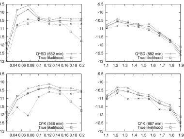
![Figure 2.4:The PAC log-likelihood surfaces normalised to 0 following Li andStephens [2003].The true likelihood surfaces in the left column are those fromFigure 2.1, and the true surfaces in the right column are those from Figure 2.3.](https://thumb-us.123doks.com/thumbv2/123dok_us/9493481.455171/60.595.129.515.284.563/likelihood-surfaces-normalised-following-andstephens-likelihood-surfaces-fromfigure.webp)