Does Energy Consumption Drive Housing Sales in China?—Based on an Optimal Dynamic General Equilibrium Model and Spatial Panel Data Analysis

ISSN Online: 2162-2086 ISSN Print: 2162-2078

Does Energy Consumption Drive Housing Sales

in China?

—Based on an Optimal Dynamic General Equilibrium Model and Spatial

Panel Data Analysis

Zhipeng Du

_{, Weikun Zhang}

_{, Yiming He}

1_{College of Economics & Management, South China Agricultural University, Guangzhou, China}

2_{National School of Agricultural Institution & Development, South China Agricultural University, Guangzhou, China}

3_{Division of Resource Management, West Virginia University, Morgantown, WV, USA}

Abstract

This paper examines the housing sales in China from 2004 to 2015 utilizing an optimal dynamic general equilibrium theoretical framework combined with a macroeconomic model. The spatial panel econometric empirical re-sults suggest that energy consumption has increased housing sales in China. However, since house is considered as a special commodity in China, and housing prices show positive impacts on housing sales.

Keywords

Energy Use, Housing Values, Optimal Dynamic General Equilibrium, Spatial Panel Econometrics, China

1. Introduction

There are many studies on energy consumption [1] or urban housing prices in China [2] [3] [4] [5] [6], but not many that examine the nexus between energy consumption and housing sales. So, the objective of the paper is to examine the relationship between them. In this paper, we focus on the impact of energy con-sumption on housing sales in the optimal dynamic general equilibrium, in China from 2004 to 2015, applying panel data OLS and panel data spatial auto regres-sion these two econometric approaches.

Currently, more and more scholars start to discuss the nexus between energy and housing issue. According to the mandatory energy performance certificates of the 2009-2010 in the Swedish private housing transactions [7] find that energy How to cite this paper: Du, Z.P., Zhang,

W.K. and He, Y.M. (2018) Does Energy Consumption Drive Housing Sales in Chi-na? Theoretical Economics Letters, 8, 3548-3566.

https://doi.org/10.4236/tel.2018.815218

Received: November 20, 2018 Accepted: December 7, 2018 Published: December 10, 2018

Copyright © 2018 by authors and Scientific Research Publishing Inc. This work is licensed under the Creative Commons Attribution International License (CC BY 4.0).

http://creativecommons.org/licenses/by/4.0/ Open Access

performance is associated with transaction price in situations when it is condi-tional on a reference benchmark. They also document property price premiums for energy performance within housing segments built before 1960 and those with a lower transaction price per square meter, meaning that the property market values energy performance, so housing segments need policy support to encourage energy improvements.

As we know, in many developed countries, wind turbines are constructed as part of a strategy to reduce dependence on fossil fuels. Using a differ-ence-in-differences methodology with a unique Dutch house price dataset cov-ering the period 1985-2011, Dröes and Koster [8] find a 1.4% price decrease for houses within 2 km of a turbine in the Netherlands. The effect is larger for taller turbines and in urban areas. Especially the first turbine built close to a house has a negative effect on its price. Meanwhile, an analysis of the private rental seg-ment reveals that, in contrast to the general market, low-Energy Performance Certificate (EPC) rated dwellings were not traded at a significant discount. This suggests different implicit prices of potential energy savings for landlords and owner-occupiers [9].

Obviously, the nexus between energy consumption and housing sales has not been pay attention to, according to the literature above. Hence, the theoretical and empirical contributions of this paper are that we utilize the Keynesian Op-timal General Equilibrium Model and Panel Spatial Econometric Approach to analyze the effect of energy consumption on housing sales in China.

The structure of this paper is as follows. This introduction section provides a brief overview of prior research analyzing the housing prices and energy con-sumption. In Section 2, we set up the optimal dynamic general equilibrium theoretical model with the energy variable and combining the macroeconomic model in the determination of the sales of housing on province level. In Section 3, we present the data utilized in the analysis and introduce the econometric methods employed. The impacts on metropolitan housing sales are examined in Section 4 and Section 5 presents conclusions and further discussion.

2. Optimal Dynamic General Equilibrium Model with Energy

and Housing Sector

2.1. Social Welfare Dynamic Optimization

In our optimal dynamic general equilibrium model, we assume the total social welfare maximization problem is expressed as below:

(

)

, ₀

max ,

t s t s

s

t t s t s

h+ c+V _s

β

∞

+ + =

=

_∑

where Vt represents the total social welfare from period 0 to infinite,

β

(

θ

)

represents the discount rate, U represents the social welfare function, ht+s

represents the housing consumption at the period (t + s), and ct+s represents

other consumption except housing consumption. Given the law of diminishing marginal utility, the social welfare function has the property of strict

si-concave, which means U Ucc, hh≤0 and U Ucc, hh ≤0.

Suppose the accumulation equation of housing can be expressed as follows:

1

t t t

h₊ S γh

∆ = + ₍₂₎

where St denotes the capacity of the real estate at the t period, and γ denotes

the value-added rate. Furthermore, considering the budget constraints of the so-ciety being expressed as:

1 h

t t t t t t t t t

a+ c p h x r a w L

∆ + + = + + ₍₃₎

where ∆at+1 represents the financial assets purchased at the (t + 1) period, pth

represents the price of the house at the t period, xt represents the dividend

in-come, rt and at respectively represent the interest rate of financial assets at

the t period and the stock of financial asset at the t period. wt represents the

wage at the t period and Lt represents the number of labor at the t period.

According to the Equations (1), (2) and (3), we can set up the Hamiltonian function:

(

)

(

)

t s t s t s t s t s t s t s t s t s t s

h

t s t s

H U c h x r a w n c p h

p h λ γ + + + + + + + + + + + + + = + + + − −

+ + (4)

The first order conditions are as below:

, 0

c t s t s

U ₊ −λ₊ = (5)

(

)

, h 1 1 h 1 0

h t s t s t s t s t s

U ₊ +λ₊ p₊ +γ −λ_{+ −} p_{+ −} = ₍₆₎ Combining (5) and (6), we obtain:

(

)

+ = ₍₇₎

And the approximate solution of optimal housing consumption utility is ex-pressed:

1

, 1 , 1 1 1

h

h t

h t c t t h

t

p

U U p

p γ

+

+ + +

 ∆ 

= − − − 

  (8)

Suppose the social welfare function takes the Cobb-Douglas form:

(

)

t t t t

U c h ₌c hα −α _{< <α (9)}

1 1

1 1 1

h

t t

h h

t t t

c p

p h p

α _γ α + + + +   = − − 

−   (10)

(

)

2.2. Energy Firm Production

Suppose the total output in the society is the function of labor and energy input.

(

)

t t t

Y F EC L= ₍₁₂₎ where ECt denotes the stock of energy used at period t, so the accumulated

energy use equation is: ∆ECt+1 = −it δECt, it denotes the flow of energy

con-sumed or investment on energy extraction at period t and δ _{denotes average} extraction cost of energy.

In the profit maximization equilibrium point, the first order condition re-quires the wage is identical to the marginal output of labor, and the marginal output of energy is identical to the extraction cost of the energy:

,

n t s t

F + =w (13)

,

EC t s

F + =δ (14) Given energy stocks and specific technical level, higher real wages will in-crease labor demand. Similarly, the demand for energy is 1

( )

, 1

k t

F− δ

+ , and the

flow of energy equation can be expressed:

( ) (

)

1

, 1 1

t k t t

i F− δ δ EC

+

= − − ₍₁₅₎

2.3. The Real Estate Sector

We assume the demand for real estate is a negatively sloped linear function as follows:

(

)

h

t t

h = +g kp k< ₍₁₆₎ The Equation (16) can be expressed as follows:

h h t

t t t h g

kp h g p k

− = − ⇒ =

On the other hand, the supply function can be expressed as:

0 1

h

t t

p =C C S+ (17) where C0 represents fixed cost due to the real estate construction and C1 represents the marginal cost of real estate for construction. Combining (16) and (17), we have

*

0 1

t t

h = +g kC C kS+ ₍₁₈₎ The difference equation which describes the housing capacity as a function of time is obtained by equating “come in market” minus “come out market” with the impact on the housing capacity, namely,

(

)

1 1

t t t

S+ =R + −s h (19)

where Rt is new building entering the housing market, s is return flow into

market coefficient. From (18) and (19), we have

(

)(

)

(

)

(

)

(

)

1 0 1

1 0

1

1 1 1

t t t

t t

S R s g kC C kS

R s C kS s g s kC

+ = + − + +

= + − + − + − (20)

(

)

(

) (

)

1 1 1 1 1 0

t t t

S+ s C kS R s g s kC

⇒ + − = + − + − ₍₂₁₎

The solution of (21) is as below:

(

)

(

)

(

)

(

)

(

)

(

)

(

)

R s g s kC

S S s C k

s C k R s g s kC

s C k

 + − + −  =_ − _{ } − _ + −     + − + − + + − (22)

Combining (18) and (22), we have:

(

)

(

)

(

)

(

)

(

)

(

)

(

)

1 0 1

1 0 1 0 1 1 1 1 1 1 1 1 1 1 t t t t

R s g s kC

h C k S s C k

s C k R s g s kC

C k g kC

s C k

 + − + −  =  − _{+ −  } − _     + − + − + + + + − (23)

Similarly, combining (17) and (22), we have:

(

)

(

)

(

)

(

)

(

)

(

)

(

)

1 0 1

1

0

1 0 0

1 1 1 1 1 1 1 1 1 1 t t h t t

R s g s kC

p C S s C k

s C k R s g s kC

C S C

s C k

 + − + −  =  − _{+ −  } − _      + − + −  +  − _{+ −} +     (24)

It is assumed that the total output function is a b

t t t t

Y u EC L= _{, and} u_t is the level of industrialization at t period, which is transferred into logarithmic form:

lnY a EC b Lt = ln t+ ln t +lnut (25)

Let NXt denote the net export, the total consumption is:

1

1

h

h h t h h

t t t t t t h t t t t t

t

p

TC c h p NX p p h h p NX

p α _γ α ₋ = +   +  +  + = +

− (26)

According to the national income equity with the government expenditure (Gt), we have

( )

(

) (

)

t t t t

h

h t h

t h t t t

t

k t t t

Y TC i G

p

p p h NX

p

F r EC G

α _γ α δ δ − − + = + +   = ₋ + +  +     +      − − +  + (27)

When the economy system reaches the steady state, the (27) is expressed as:

( )

( )

(

)

2 ₁

, 1 1

ln ln ln ln

1

ln 1 ln

h

h t h

t t h t t k t

t

t t

p

Y p p h F

p

EC G

α _{γ δ}

α δ − + −       =  ₋  + + + + _{ }       − _ − _+ (28)

The Equation (28) is further transformed into:

(

) (

)

( )

( )

(

)

ln 1 ln ln ln ln 1

1

ln ln 1 ln ln

h

h t

t t t t t h

t

k t t t

p

h a EC b L u p

p

F G NX

α _γ α δ δ − − +     = + + + −  ₋  + +          − _{ }− − − − (29)

The Equation (29) will be used to explain the rapid rise in the sales of housing in China. So, from Equation (29), the effect mechanism of energy consumption on equilibrium housing sales can be derived:

(

)

ln ₁

ln tt h

a EC

∂ _{= +}

∂ (30)

So, an important hypotheses stem from Equation (30):

Hypothesis: Energy consumption is positively related with housing sales in

China.

3. Data Description and Econometric Methodology

3.1. Data

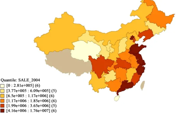
In order to test the effect of energy consumption on housing sales above, we uti-lized data from China and conduct this analysis at the province level. However, we exclude the data from Tibet province, because of the problem of data miss-ing. Hence, there are 30 provinces in our sample. Panel data from 2004 to 2015 were obtained from the China statistical yearbook from 2005-2016 and the Chi-na Stock Market & Accounting Research (CSMAR) Database and EPS database. The spatial distribution of housing sales of China in 2004 and 2015 are listed in

Figure 1 and Figure 2.

Figure 1. Hot bitmap of housing sales of China in 2004.

Figure 2. Hot bitmap of housing sales of China in 2015.

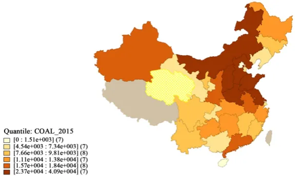
Similarly, the spatial distribution of coal consumption of China in 2004 and 2015 are listed in Figure 3 and Figure 4.

The description and definition of variables are shown in Table 1. The statistical description is demonstrated in Table 2.

Figure 3. Hot bitmap of coal consumption of China in 2004.

Figure 4. Hot bitmap of coal consumption of China in 2015.

Table 1. Mnemonic and variable definition.

Variable Mnemonic Definition Expected _direction

housing sales ltsale ltsale = ln(housing sales)

coal consumption lcoal local = ln(coal consumption) + average price of house laprice laprice = ln(average price of house) + employment in housing sector lem lem = ln(em) + industrialization lur lur = ln(non-agricultural output/GDP) + net export lnx lnx = ln(export-import) - local government expenditure lg lg = ln(local government expenditure) -

Table 2. Variables descriptive statistics.

Variable Obs Mean Std. Dev. Min Max Skewness Kurtosis lsale 360 15.78512 1.24224 11.68179 18.41741 −0.54273 2.904726 lcoal 360 9.066617 0.909592 5.786928 10.61954 −0.9167 4.337971 laprice 360 10.20024 0.668059 8.346405 11.58952 −0.14927 2.402243 lur 360 4.478663 0.070334 4.144832 4.600789 −0.80762 5.206171 lem 360 10.92285 0.753468 8.394347 12.34112 −0.79331 3.644049 lg 360 7.201438 0.881996 4.673856 9.189754 −0.44411 3.028859 lnx 360 6.56454 11.51134 −17.226 17.0883 −1.12129 2.387432

To describe the statistical characteristics among the variables, the scatter fit-ting figure is utilized. Figure 5 depicts the scatter fitting plot between coal con-sumption and housing sales, Figure 6 depicts the scatter fitting plot between industrialization and housing sales, and Figure 7 depicts the scatter fitting plot between housing prices and housing sales. They all demonstrate that housing sales, coal consumption, industrialization, and housing prices increase together respect to time.

3.2. Econometric Model Design and Specification

3.2.1. Panel unit Root Model

A standard individual ADF test was conducted on stationary panel data [10].

Following this line of analysis, we first test the unit roots of yit to confirm the

sta-tionary properties for each variable. This was achieved by using the Im-Pesaran- Shin (IPS) test [11]. In order to verify the robustness of the sequence, we used IPS method to test the heterogeneity of panel unit root, the advantages of this method is not only consider the heterogeneous panels, but also consider the is-sues about serial correlation.

, 1 1 , , 1,2, , ; 1,2, ,

pi

it i i t L iL i t L it i it

y

ρ

β

γ

∆ = +

∑

where, y = {lsale, lcoal, laprice, lem, lur, lnx} is 5 * 1 dimensional vector, zit′ is a

temporal trend term, γi is the coefficient vector, it is the error term and

satis-fies the independent normal distribution.

3.2.2. Panel Data OLS Regression and Fixed Effect Model

Since the fixed effect regression comes from the OLS panel model, we firstly in-troduce the latter:

(

)

i

it it i it

ltsale =x′

β

δ µ ε

con-trolled variables (lg, lem, lnx); the observable random variable zi represents the

intercept term of individual heterogeneity such as customs, culture, location, etc., disturbance term is composited by µ εi+ it, which is also called composite

error term. Unobservable random variable µi represents the intercept term of

individual heterogeneity, and εit is the perturbation term varying with the

in-dividual and time. It is generally assumed that εit is independent and identically

Figure 5. Scatter fitting plot between local and lsale.

Figure 6. Scatter fitting plot between lur and lsale.

Figure 7. Scatter fitting plot between laprice and lsale.

2004

2005 2006

2007 2008

2009

2010 2011 2012

2013₂₀₁₄2015

18

.5

19

19

.5

20

20

.5

12.2 12.4 12.6 12.8 13

lcoal

lsale Fitted values

2004 2005

2006 2007

2008 2009

20102011 2012

201320142015

18

.5

19

19

.5

20

20

.5

21

3.7 3.8 3.9 4 4.1

lur

lsale Fitted values

2004

2005 2006

2007 2008

2009

2010 2011 2012

2013 2014

2015

18

.5

19

19

.5

20

20

.5

8 8.2 8.4 8.6 8.8

laprice

lsale Fitted values

distributed, and is not related to µi. The pooled OLS model and fixed effect

model are based on (32). The pooled OLS regression assumes that all individuals have a consistent regression equation, and the model (33) is transferred as fol-lows:

(

)

it it i it

ltsale = +

α

β

δ ε

For the fixed effect model, given the individual i, the mean value of the Equa-tion (33) respect to time t is as below:

(

)

i

it it i it

ltsale =x′β+z′δ µ ε+ + i=  n t=  T (34)

Then, the Equation (32) minus the mean Equation (34), so we obtain:

(

) (

)

it it it it it it

ltsale ltsale− = x −x′ ′β+ ε −ε ₍₃₅₎

Next, we define ltsaleit =

(

)

(

)

(

)

 _{it it} _it

ltsale =x ′β ε+ ₍₃₆₎

In (36), µi can be eliminated, so if

ε

be used to estimate consistent estimates

β

3.2.3. Spatial Panel Data Econometric Model

In order to measure the spillover effect of housing sales, the spatial panel data econometric model generally can be expressed as [12] [13]:

, 1

it i t i t i i i i it

y =τy − +ρw y d X′ + ′ δ µ γ+ + +ε

it mi i it

ε =λ ε ν′ +

where, wi′ is the ith row in spatial weight matrix W i j

( )

n

i t j ij jt

w y′ =

∑

( )

spa-tial lagged term; y is the dependent variable(ltsale), X is the vector of indepen-dent variables (local, laprice, lem, lex, lg, lur), µi is the individual effect among

the provinces; γi is the time effect among the provinces; mi′ is the disturbing

term at the ith row in spatial weight matrix.

If λ=0 _and δ =0_{, we will have the spatial autoregressive model. If} τ=0 and δ =0_{, we will have the spatial autocorrelation model. If}

τ ρ

0

δ = _{, we will have the spatial error model.}

3.2.4. Spatial Autocorrelation and Moran Index

Spatial weight matrix is the requirement to use spatial econometric analysis. Based on the spatial distance between provinces and according to the spatial dis-tribution of the variables, we construct the spatial weight matrix. The method to construct matrix is that if two provinces are adjacent, and the value of element in the spatial weight matrix is identical to 1. Otherwise, the value of element in the spatial weight matrix is identical to 0. Then through the Moran index, we could measure the spatial dependence of the spatial panel data. The Moran index is as follows [14]:

(

)

(

)

(

)

(

)

1 1

2

1 1 1

n n

ij i j

i j

n n n

ij i

i j i

n x x x x

I

x x

ω ω

= =

= = =

− −

=

−

∑ ∑

∑ ∑

∑

where 1 n₁ i

j x

x

n =

=

∑

province, ωij is the value of element in spatial weight matrix from the ith province to the jth province. Moran index ranges from [−1, 1]. If I is closer to 1, it means the stronger positive spatial correlation. If I is close to −1, it means the negative spatial correlation is stronger. If I is closer to 0, it means spatial correla-tion does not exist. Moran index can be regarded as the coefficient of correlacorrela-tion between the spatial lag and the value of observation. If the observation value and the spatial lag are drawn scatter diagram, namely Moran scatterplot, the Moran index I is the slope of the regression line of the scatter.

4. Empirical Results

4.1. Unit Root Test

We use individual ADF test to identify the unit root process. The null hypothesis is that the variable is nonstationary. The results in Table 3 show that local, lur, lg and lem are stationary at one percent significant level, and ltsale, laprice, and lnx are stationary at five percent significant level.

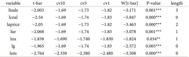
In terms of the IPS test, the null hypothesis is that the panel series are nonsta-tionary. The test results are shown in Table 4. ltsale, laprice, local, lur, lg, and lem are stationary at one percent significant level, and lnx is stationary at five percent significant level.

Table 3. Individual ADF test results.

variable t-bar cv10 cv5 cv1 Z[t-bar] P-value length ltsale −2.098 −2.07 −2.15 −2.32 −1.923 0.027** 1 lcoal −5.055 −2.07 −2.17 −2.34 −16.603 0.000*** 2 laprice −2.153 −2.07 −2.15 −2.32 −2.215 0.013** 0 lur −2.24 −2.07 −2.17 −2.34 −2.589 0.005*** 2 lnx −2.106 −2.07 −2.17 −2.34 −1.92 0.027** 0 lg −4.542 −2.07 −2.17 −2.34 −14.052 0.000*** 2 lem −2.274 −2.07 −2.17 −2.34 −2.759 0.003*** 0 Note: *indicates 10% critical value, **indicates 5% critical value and ***indicates 1% critical value.

Table 4. IPS test results.

variable t-bar cv10 cv5 cv1 W[t-bar] P-value length ltsale −2.003 −1.69 −1.73 −1.82 −3.171 0.001*** 3 lcoal −2.54 −1.69 −1.74 −1.83 −5.847 0.000*** 0 laprice −2.05 −1.69 −1.73 −1.82 −3.463 0.000*** 2 lur −2.068 −1.69 −1.74 −1.83 −3.078 0.001*** 1 lnx −1.838 −1.690 −1.740 −1.830 −1.824 0.034** 1 lg −1.965 −1.69 −1.74 −1.83 −2.572 0.005*** 0 lem −2.764 −2.330 −2.380 −2.480 −3.508 0.000*** 0 Note: *indicates 10% critical value, **indicates 5% critical value and ***indicates 1% critical value.

4.2. Spatial Autocorrelation Test Results

According to the Moran index of housing sales from 2004 to 2015 in China, as shown in Figure 8, there is significant spatial autocorrelation in the sample, be-cause the Moran index is greater than zero and less than one.

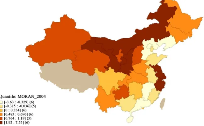
Additionally, the spatial distribution of Moran index of the housing sales of China in 2004 and 2015 are listed in Figure 9 and Figure 10.

Similarly, the spatial distribution of Moran index of the coal consumption of China in 2004 and 2015 are listed in Figure 11 and Figure 12.

Figures 9-12 all demonstrate that some provinces in deep red can reject the null hypothesis of non-spatial auto correlation, which is consistent with the global spatial auto correlation test result.

Figure 8. The Moran index of housing sales from 2004-2015.

Figure 9. Hot bitmap of Moran index of housing sales in 2004.

Figure 10. Hot bitmap of Moran index of housing sales in 2015.

Figure 11. Hot bitmap of Moran index of coal consumption in 2004.

Figure 12. Hot bitmap of Moran index of coal consumption in 2015.

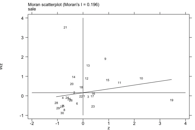
In addition, the Moran scatterplot of housing sales of China in 2004 and 2015 is listed in Figure 13 and Figure 14. Figure 13 and Figure 14 show that, the spatial correlation Moran index of housing sales in China decrease from 0.203 (in 2004) to 0.196 (in 2015), which means that the global spatial auto correlation of housing sales in China becomes weaker respect to time.

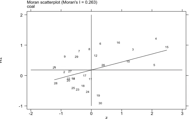
Similarly, the Moran scatterplot of coal consumption of China in 2004 and 2015 is listed in Figure 15 and Figure 16. Figure 15 and Figure 16 show that, the spatial correlation Moran index of coal consumption in China decrease from 0.203 (in 2004) to 0.196 (in 2015), which means that the global spatial auto cor-relation of coal consumption in China becomes weaker respect to time, too.

Figure 13. Moran scatterplot of housing sales of China in 2004.

Figure 14. Moran scatterplot of housing sales of China in 2015.

Moran scatterplot (Moran's I = 0.203) sale

Wz

z

-1 0 1 2 3 4

-1 0 1 2

28 21

27₂₉4 247

5 30 2625

14 3

8 18 16 20

22 12

17 2

23 13

6 15

11 10

19 1

9

Moran scatterplot (Moran's I = 0.196) sale

Wz

z

-2 -1 0 1 2 3 4

-1 0 1 2 3 4

28 2927

30 7 4 5 8 21

242526 20 14

2 6

22 18 1

12 13

3 17 23 16

9

15 11

10

19

Figure 15. Moran scatterplot of coal consumption of China in 2004.

Figure 16. Moran scatterplot of coal consumption of China in 2015.

4.3. Regression Results

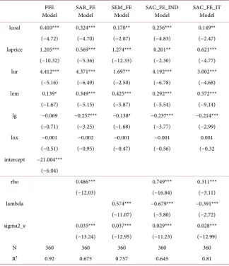
Since different models have different advantages and characteristics, and in or-der to ensure the robustness of the results, fixed effects panel model (PFE), spa-tial autoregression model (SAR), spaspa-tial error model (SEM), the spaspa-tial autocor-relation model (SAC) are utilized. In the SAR model, individual (SAR-IND) and individual-time (SAR-IT) these two types of model are considered, respectively.

Table 5 shows coal consumption is positively related to housing sales at one percent significant level in the PFE Model, SAR_FE Model, and, SAC_FE_IND Model. Meanwhile, the coefficient of coal consumption is positive and signifi-cant on five percent in SEM_FE Model and SAC_FE_IT Model. So, the hypothe-sis about the nexus between coal consumption and housing sales cannot be re-jected.

Moran scatterplot (Moran's I = 0.314) coal

Wz

z

-2 -1 0 1 2 3

-2 -1 0 1 2

21

28 2922

1 20

27 2

30 1314

26 9

25 7

18 8

12

24 17 23

11 19

5 6

10 16

3 15

4

Moran scatterplot (Moran's I = 0.263) coal

Wz

z

-2 -1 0 1 2 3

-1 0 1 2

211

28 2 9

20 22 27

13 14 25 29

23 7

18 17

24 8

11 12

19 6

30 26

16

10 3

5 4

15

Table 5. Regression results (ltsale as dependent variable).

PFE

Model SAR_FE Model SEM_FE Model SAC_FE_IND Model SAC_FE_IT Model lcoal 0.410*** 0.324*** 0.170** 0.256*** 0.149**

(−4.72) (−4.70) (−2.07) (−4.83) (−2.47) laprice 1.205*** 0.569*** 1.274*** 0.201** 0.621*** (−10.32) (−5.36) (−12.33) (−2.30) (−4.77) lur 4.412*** 4.371*** 1.697** 4.192*** 3.002*** (−5.16) (−6.49) (−2.50) (−6.78) (−4.68) lem 0.139* 0.349*** 0.425*** 0.292*** 0.572*** (−1.67) (−5.15) (−5.87) (−5.54) (−9.14) lg −0.069 −0.257*** −0.138* −0.237*** −0.214***

(−0.71) (−3.25) (−1.68) (−3.77) (−2.99) lnx −0.001 −0.002 −0.001 −0.001 0.001

(−0.51) (−0.95) (−0.47) (−0.56) (−0.32 intercept −21.004***

(−6.04)

rho 0.486*** 0.749*** 0.311***

(−12.03) (−16.84) (−3.11) lambda 0.574*** −0.679*** −0.391***

(−11.07) (−5.80) (−2.72) sigma2_e 0.035*** 0.037*** 0.029*** 0.028*** (−13.24) (−12.95) (−11.23) (−12.99)

N 360 360 360 360 360

R2 _{0.92 0.675 0.757 0.645 0.81}

Notes: 1) t statistics in parentheses. 2) *indicates 10% critical value, **indicates 5% critical value and ***indicates 1% critical value.

Furthermore, the coefficient of housing prices is positive significant, which is consistent with the statement derived from Equation (10). Since Equation (10),

we have

(

)

(

)

( ) (

)

1 1 1 1

1

2 2

1 _{1 1 1}

1 1

0 1

h h h h

t t t t t t

t

h _{h h h h}

t _{t t t t t}

c p p r p p

h

p _{p p r p p}

α γ

α γ

+ + + +

+

+ _{+ + +}

 

− − + − −

∂ ₌  _>

∂ _{+ − −} . Actually, in

China, the housing prices bubbles demonstrate inter-provincial spillover effect

[15], urbanization [16], local government’s land hoarding behavior [17], local governments’ budget deficit [18], income rises [19] and monetary policy impact

[20] have led to a strong demand for housing in urban China [21]. So, the hous-ing sales would rise, which is consistent with the positive relationship between housing prices and housing sales.

5. Conclusions

To analyze the nexus between coal consumption and housing sales in China, an optimal dynamic general equilibrium model is setup including energy and

housing sector. The empirical results indicate housing sales is positively corre-lated with the energy consumption and is positively correcorre-lated with housing prices. That outcome is similar to what has been documented in previous studies conducted using national level data for European countries, such as Wales, Sweden and Holland. It is instructive that, during a period of rapid industrializa-tion, energy is found to represent a crucial factor undergirding economic growth

[22]. This suggests that housing sales in developing countries may require eco-nomic growth and so energy generation as necessary pre-condition for expan-sion.

Indeed recent decades have seen a decoupling of GDP growth and energy consumption at the metropolitan level [23]. Gains in energy efficiency and con-sumption in the sectoral composition of total output have allowed housing sales to grow at a slower pace than GDP. An upward trend in housing sales has been observed in China from 2004 to 2015, suggesting that ever-increasing housing sales are not an indispensable corollary of regional energy consumption. Some scholars suggest the Chinese government should impose the property tax to control the housing prices bubbles [24], but according our theoretical and em-pirical findings, the housing prices control means housing sales regulation. However, the first-tier city bubble may not burst due to the urbanization process

[25], hence, the housing sales and housing prices in China both dramatically go up, recently.

Future research avenues include development of the continued variable op-timal dynamic stochastic general equilibrium of the nexus among housing pric-es, energy consumption, and economic growth. This model would require an in-depth analysis of dynamic optimization of housing prices along with specially developed non-linear energy consumption function in China [26]. In addition, a similar empirical framework could be extended by using a spatial difference- in-difference panel econometric model [15]. This model would require an in-depth analysis of the institutional effect of regional energy policy on housing prices and housing sales [16]. Finally, natural experiment coverage could be conducted to examine the nexus among energy consumption, housing prices and housing sale after and prior to national energy policy between the control regional group and treatment regional group [17]. This strategy would enable researchers to investigate whether or not housing prices and housing sales are altered when energy intensity is improved [27].

Acknowledgements

This work was supported by National Ten Thousand Outstanding Young Scho-lar Program (Grant Number: W02070352) as well as Key Project of National Natural Science Foundation in China, (Grant Number: 71742003).

Conflicts of Interest

The authors declare no conflicts of interest regarding the publication of this pa-per.

References

[1] He, Y.M. and Gao, S.H. (2017) Economic Growth, Urbanization, Industrialization,

and Metropolitan Electricity Consumption: Evidence from Guangzhou in China.

The Empirical Economics Letters, 16, 195-208.

[2] Ho, M.HC. and Kwong, T.M. (2002) Housing Reform and Home Ownership

Beha-viour in China: A Case Study in Guangzhou. Housing Studies, 17, 229-244.

https://doi.org/10.1080/02673030220123207

[3] Jim, C.Y. and Chen, W.Y. (2006) Impacts of Urban Environmental Elements on

Residential Housing Prices in Guangzhou (China). Landscape and Urban Planning,

78, 422-34. https://doi.org/10.1016/j.landurbplan.2005.12.003

[4] Jim, C.Y. and Chen, W.Y. (2007) Consumption Preferences and Environmental

Ex-ternalities: A Hedonic Analysis of the Housing Market in Guangzhou. Geoforum,

38, 414-431. https://doi.org/10.1016/j.geoforum.2006.10.002

[5] Wang, D.G. and Li, S.M. (2006) Socio-Economic Differentials and Stated Housing

Preferences in Guangzhou, China. Habitat International, 30, 305-326.

https://doi.org/10.1016/j.habitatint.2004.02.009

[6] Li, S.M. (2010) Mortgage Loan as a Means of Home Finance in Urban China: A

Comparative Study of Guangzhou and Shanghai. Housing Studies, 25, 857-876.

https://doi.org/10.1080/02673037.2010.511154

[7] Cerin, P., Hassel, L.G. and Semenova, N. (2014) Energy Performance and Housing

Prices. Sustainable Development, 22, 404-419. https://doi.org/10.1002/sd.1566

[8] Dröes, M.I. and Koster, H.R.A. (2016) Renewable Energy and Negative

Externali-ties: The Effect of Wind Turbines on House Prices. Journal of Urban Economics,

96, 121-141. https://doi.org/10.1016/j.jue.2016.09.001

[9] Fuerst, F., McAllister, P., Nanda, A. and Wyatt, P. (2016) Energy Performance

Rat-ings and House Prices in Wales: An Empirical Study. Energy Policy, 92, 20-33.

https://doi.org/10.1016/j.enpol.2016.01.024

[10] Pesaran, M.H. (2007) A Simple Panel Unit Root Test in the Presence of Cross-Section

Dependence. Journal of Applied Econometrics, 22, 265-312.

https://doi.org/10.1002/jae.951

[11] Im, K.S., Pesaran, M.H. and Shin, Y. (2003) Testing for Unit Roots in

Heterogene-ous Panels. Journal of Econometrics, 115, 53-74.

https://doi.org/10.1016/S0304-4076(03)00092-7

[12] Anselin, L. and Arribas-Bel, D. (2013) Spatial Fixed Effects and Spatial Dependence

in a Single Cross-Section. Papers in Regional Science, 92, 3-17.

https://doi.org/10.1111/j.1435-5957.2012.00480.x

[13] Anselin, L. and Lozano-Gracia, N. (2008) Errors in Variables and Spatial Effects in

Hedonic House Price Models of Ambient Air Quality. Empirical Economics, 34,

5-34. https://doi.org/10.1007/s00181-007-0152-3

[14] Li, H.F., Calder, C.A. and Cressie, N. (2007) Beyond Moran’s I: Testing for Spatial

Dependence Based on the Spatial Autoregressive Model. Geographical Analysis, 39,

357-375. https://doi.org/10.1111/j.1538-4632.2007.00708.x

[15] Shih, Y.N., Li, H.C. and Qin, B. (2014) Housing Price Bubbles and Inter-Provincial

Spillover: Evidence from China. Habitat International, 43, 142-151.

https://doi.org/10.1016/j.habitatint.2014.02.008

[16] Chen, J., Fei, G. and Ying, W. (2011) One Decade of Urban Housing Reform in

China: Urban Housing Price Dynamics and the Role of Migration and Urbaniza-tion, 1995-2005. Habitat International, 35, 1-8.

https://doi.org/10.1016/j.habitatint.2010.02.003

[17] Du, J. and Peiser, R.B. (2014) Land Supply, Pricing and Local Governments’ Land

Hoarding in China. Regional Science and Urban Economics, 48, 180-189.

https://doi.org/10.1016/j.regsciurbeco.2014.07.002

[18] Wu, G.L., Feng, Q. and Li, P. (2015) Does Local Governments’ Budget Deficit Push

up Housing Prices in China? China Economic Review, 35, 183-196.

https://doi.org/10.1016/j.chieco.2014.08.007

[19] Feng, Q. and Wu, G.L. (2015) Bubble or Riddle? An Asset-Pricing Approach

Evalu-ation on China’s Housing Market. Economic Modeling, 46, 376-383.

https://doi.org/10.1016/j.econmod.2015.02.004

[20] Ng, E.C.Y. (2015) Housing Market Dynamics in China: Findings from an Estimated

DSGE Model. Journal of Housing Economics, 29, 26-40.

http://linkinghub.elsevier.com/retrieve/pii/S1051137715000315

https://doi.org/10.1016/j.jhe.2015.05.003

[21] Yao, S., Luo, D. and Wang, J. (2014) Housing Development and Urbanisation in

China. World Economy, 37, 481-500.https://doi.org/10.1111/twec.12105

[22] He, Y. and Gao, S. (2017) Gas Consumption and Metropolitan Economic

Perfor-mance: Models and Empirical Studies from Guangzhou, China. International

Jour-nal of Energy Economics and Policy, 7, 121-126.

[23] He, Y., Fullerton, T.M. and Walke, A.G. (2017) Electricity Consumption and

Met-ropolitan Economic Performance in Guangzhou: 1950-2013. Energy Economics, 63,

154-160.https://doi.org/10.1016/j.eneco.2017.02.002

[24] Du, Z. and Zhang, L. (2015) Home-Purchase Restriction, Property Tax and Housing

Price in China: A Counterfactual Analysis. Journal of Econometrics, 188, 558-568.

https://doi.org/10.1016/j.jeconom.2015.03.018

[25] Liu, T.Y., Chang, H.L., Su, C.W. and Jiang, X.Z. (2016) China’s Housing Bubble

Burst? Economics of Transition, 24, 361-389.https://doi.org/10.1111/ecot.12093

[26] Wang, S.-Y. (2011) Misallocation and Housing Prices: Theory and Evidence from

China. The American Economic Review, 101, 2081-2107.

http://www.jstor.org/stable/23045631

[27] Chow, G.C. and Niu, L. (2015) Housing Prices in Urban China as Determined by

Demand and Supply. Pacific Economic Review, 20, 1-16.

https://doi.org/10.1111/1468-0106.12080