A local scale sensitive indicator of spatial autocorrelation for assessing high and low value clusters in multiscale datasets

warwick.ac.uk/lib-publications Manuscript version: Author’s Accepted Manuscript

The version presented in WRAP is the author’s accepted manuscript and may differ from the published version or Version of Record.

Persistent WRAP URL:

http://wrap.warwick.ac.uk/114593

How to cite:

Please refer to published version for the most recent bibliographic citation information. If a published version is known of, the repository item page linked to above, will contain details on accessing it.

Copyright and reuse:

The Warwick Research Archive Portal (WRAP) makes this work by researchers of the University of Warwick available open access under the following conditions.

Copyright © and all moral rights to the version of the paper presented here belong to the individual author(s) and/or other copyright owners. To the extent reasonable and

practicable the material made available in WRAP has been checked for eligibility before being made available.

Copies of full items can be used for personal research or study, educational, or not-for-profit purposes without prior permission or charge. Provided that the authors, title and full

bibliographic details are credited, a hyperlink and/or URL is given for the original metadata page and the content is not changed in any way.

Publisher’s statement:

Please refer to the repository item page, publisher’s statement section, for further information.

A local scale-sensitive indicator of spatial autocorrelation for assessing

high- and low-value clusters in multi-scale datasets

Rene Westerholt

, Bernd Resch

and Alexander Zipf

a

GIScience Research Group, Institute of Geography, Heidelberg University, Germany;

b

Z_GIS, Department of Geoinformatics, University of Salzburg, Austria; cCenter for Geographic Analysis, Harvard University, USA

Georeferenced user-generated datasets like those extracted from Twitter are increasingly gaining the interest of spatial analysts. Such datasets oftentimes reflect a wide array of real-world phenomena. However, each of these phenomena takes place at a certain spatial scale. Therefore, user-generated datasets are of multi-scale nature. Such datasets cannot be properly dealt with using the most common analysis methods, because these are typically designed for single-scale datasets where all observations are expected to reflect one single phenomenon (e.g., crime incidents). In this paper, we focus on the popular local G statistics. We propose a modified scale-sensitive version of a local G statistic. Furthermore, our approach comprises an alternative neighborhood definition that is enables to extract certain scales of interest. We compared our method with the original one on a real-world Twitter dataset. Our experiments show that our approach is able to better detect spatial autocorrelation at specific scales, as opposed to the original method. Based on the findings of our research, we identified a number of scale-related issues that our approach is able to overcome. Thus, we demonstrate the multi-scale suitability of the proposed solution.

Keywords: Scale, Spatial Autocorrelation, User-Generated Data, Social Media, Twitter

1. Introduction

Spatial patterns of geographic phenomena can be explored using indicators of spatial autocorrelation. Such indicators express the degree of dependence among different observations of some spatial variable (Getis 2010). In more general terms, spatial autocorrelation can be described as the correlation between a matrix of spatial relations (usually referred to as “spatial weights matrix”) and an attribute value matrix. Corresponding indices are often designed as test statistics. In such circumstances, their goal is to find unusually high degrees of spatial dependence by testing against the null hypothesis of spatial independence (Getis 2010). Typical fields where this kind of statistic is particularly helpful are human geography, epidemiology or criminology. In such fields, spatial autocorrelation statistics can, for instance, be used for finding areas of high economic prosperity, regions of elevated infectivity or crime hot spots.

*

One recurring problem with spatial autocorrelation statistics is their sensitivity to spatial scale effects. Most geographic phenomena operate on a specific scale range. This typically includes both an upper and a lower distance bound. Some processes occur globally, while others are limited to small regions (Dungan et al. 2002). Therefore, geographic data acquisition requires adjusting the measuring scale to the phenomenon of interest. This is achievable with little effort in controlled experiments that rely on automated measuring devices. Appropriate geographic deployment of such devices leads to a correctly scaled dataset. However, adjusting the measurement scale becomes more difficult (or even impossible) when employing uncontrolled data acquisition methods, for instance when observing social activities through georeferenced human reports in social media feeds like Twitter. Such uncontrolled data acquisition does not allow for a priori scale adjusting and thus causes a potential misfit of the measuring scale. In addition, user-generated data often represents more than one phenomenon. Observations originating from such data sources reflect a wide array of underlying phenomena. Moreover, single contributors reporting about these phenomena typically do not interact directly. Thus, their contributions appear in a geometrically superimposed manner. A similar effect can be observed in census data, where processes operating at different scales are interacting crosswise and are aggregated to the respective datasets (Manley et al. 2006). The analysis of user-generated data in general is of ever increasing interest. Recently, social media in particular has been leveraged in diverse fields such as human mobility analysis (e.g., Hawelka et al. 2014), event detection (e.g., Crooks et al. 2013) or sentiment analysis (e.g., Mitchell et al. 2013).

However, most of the available spatial autocorrelation statistics have been developed in the context of controlled data acquisition processes. They assume some spatial variable to represent only one phenomenon, measured at a best fitting scale. In such case, it is possible to adopt a region-oriented point of view by asking the question “What region of a dataset is out of the ordinary?” Here, one just has to properly model the size and shape of the focal neighborhoods. However, topic and thus multi-scale datasets like those extracted from social media are of heterogeneous nature. Every sub-region can contain observations at small scales being situated next to others at larger scales. These observations appear to be crosswise and overlapping. In fact, one region cannot be regarded as one coherent spatial unit in such cases. The question here changes to “Which observation at a certain scale in what region of a dataset is out of the ordinary?” Thus, the focus changes from being purely region-oriented towards a phenomenon-oriented viewpoint. The question is how to separate the extraordinary from the ordinary without drawing wrong conclusions from such heterogeneous mixed-scale regions.

simple binary contiguity. This effect even appears across different scales (Dacey 1965). One can avoid this kind of problem by recognizing topology in the neighborhood definition via applying an appropriate weighting scheme (Cliff & Ord 1969). Another way of dealing with scale is to use local statistics instead of global measures. These can account for non-stationary spatial processes and exogenous factors causing heterogeneity (such as topography). Thus, they can model local-scale characteristics more realistically (Fotheringham 2009).

In this paper, we propose a modified version of a local G statistic, which we call GS statistic. The “S” in the name reflects our emphasis on scale. Our version of the local G statistic is able to deal with multi-scale datasets. Spatial autocorrelation can be assessed by following a two-step approach: First, the scale range of interest is extracted by relying on a new neighborhood definition. Our neighborhood definition differs from common approaches in that all tuples of observations within the local focus are examined with respect to their scale. Furthermore, the principle of the statistic itself is modified towards operating at a certain scale, instead of mixing up different ones. This allows for unraveling the autocorrelation structure of all locally available scales separately. We further develop equations for assessing the variance and the expectation and we present a standardized version of our statistic. Finally, we test our approach by comparing it to the original method. We apply both the original and our method to a Twitter dataset consisting of a snapshot of an urban setting from the city of San Francisco and we discuss some scale-related issues.

We start the remainder of this article by giving background information on the ambiguous term of geographic scale in Section 2. Afterwards, in Section 3, we present a literature review on the field of spatial autocorrelation statistics, with special focus on scale. In Section 4, we define our modified statistic, which is being tested in Section 5. We end our paper with some concluding remarks in Section 6.

2. Background: some notes on geographic scale

The concept of geographic scale is central to this paper. Spatial phenomena are supposed to operate at a certain scale. Therefore, accounting for this property is crucial for obtaining realistic results from spatial autocorrelation analysis. However, scale is an ambiguous term. While the concept is of interest to several disciplines, each adopted a different meaning (see Gibson et al. 2000 for a multi-disciplinary overview). Ecologists use the term for describing levels in the hierarchical system of biological taxonomy or in the hierarchy of a food chain (Allen & Hoekstra 1992). Sociologists classify their research according to the scale of human relationships, i.e., into micro-, meso-, macro- and global-sociology (Smelser 1995). Scholars from political sciences or from urban planning use the term “scale” less from a quantitative than a conceptual point of view. In analogy to political jurisdictions, they classify their research into studies at the local, regional, national or international scale (Turner et al. 1989, Gibson et al. 2000).

(Turner et al. 1989). In contrast, phenomenon scale (or operational scale) describes the areal magnitude that a phenomenon covers in the real world (Lam & Quattrochi 1992, Montello 2001). Its counterpart is analysis scale (or methodological scale), which denotes the unit size used for aggregation (Lam & Quattrochi 1992, Montello 2001). The concurrent term “resolution” basically describes the same concept in remote sensing, where it is used to specify the width of equally sized grid cells. Another more general description of the concept of resolution/analysis scale has been given by Waldo Tobler. He describes this concept as the representation of the smallest distinguishable parts (Tobler 1988).

Throughout the remainder of this paper, we use the term “scale” to refer either to phenomenon or analysis scale. Both are interrelated. If one is analyzing a spatial phenomenon at a wrongly adjusted analysis scale, the analyst misses out the essential information (i.e., spatial variation) (Goodchild 2001). Thus, it is crucial to harmonize the phenomenon scale (or the “real-world” scale) and the analysis scale.

3. Literature review

A broad range of indicators for measuring spatial autocorrelation has been developed over the last decades. Many of them are of global nature and describe the average spatial autocorrelation across a given region. Popular examples include the autocovariance-based Moran’s I (Moran 1950), the semivariance-based Geary’s C (Geary 1954) or Tango’s C (Tango 1995) and Rogerson’s R (Rogerson 1998), the two latter being both related to the 𝜒²-goodness-of-fit test. A statistic that moreover allows statements about the characteristics of the involved observations is Getis & Ord’s G (Getis & Ord 1992, Getis & Ord 1995). Zhang & Lin (2006) modified G for overcoming the problem whereby high and low values might cancel each other out. These authors also presented an alternative approach to G by decomposing Moran’s I into three separate statistics (Zhang & Lin 2007). These are respectively capable of finding either high-value, medium-value or low-value accumulation.

The indicators presented above are designed for dealing with numerical attribute values. However, more recently, some research has also taken place around indicating spatial autocorrelation in the context of categorical data. This kind of spatial association is indeed beyond the focus of this paper. However, some recent examples can be found in Boots (2003), Ruiz et al. (2010) and Leibovici et al. (2014). Most of these indicators are based on entropy measures.

1995) or local R (Rogerson 1998). The general principle of these statistics is to compare a local neighborhood to some overall dataset. However, this is problematic when considering the potential heterogeneity of spatial regions with respect to underlying covariates. A recent approach that has been presented by Ord & Getis (2001) tries to overcome this issue by comparing contiguous regions instead.

The compilation of spatial weights matrices is another strategy for dealing with scale issues. Aldstadt & Getis (2004) revealed at least eleven different schemes for this purpose. Getis (2009) categorized them into three categories according to their respective nature. Following this, spatial weight matrices can be constructed by following a theoretical, empirical or topological point of view. Theoretical approaches are based on some underlying distance theory such as Zipf’s law (Zipf 1949). They assume the spatial weights to be exogenous to any system. The most frequently applied approach of this kind is using some sort of inverse distance. Scale is typically modelled by inducing an upper distance bound. The opposite of the theoretical approach to constructing weight matrices is constructing them in an empirical manner. Here, the analyst tries to estimate the neighborhood structure by extracting it from some reference region of a given dataset. However, this reference region is also the limiting factor for the explanatory power of such matrices. A third approach to matrix construction is trying to depict the topology as realistically as possible. These approaches are motivated by the well-known issue of topological invariance (Dacey 1965), which leads to similar matrices across different topological settings when using binary contiguity indicators. An issue related to scale here is that differently sized spatial units are nevertheless treated similarly. Cliff & Ord (1969) suggested using suitable weighting schemes to overcome this problem. Examples of recent approaches for matrix construction include that of Getis & Aldstadt (2004) (utilization of a local statistic for assessing a proper matrix) or LeSage (2003) (Gaussian distance). Two interesting approaches with specific focus on scale are presented by Aldstadt & Getis (2006) and Rogerson & Kedron (2012). Both of them are based on successive expansions of the neighborhood size until a maximum value of a given local statistic (e.g., local Moran’s I) is reached. Another approach for finding a suitable scale is leveraging the range of local semivariograms (Lloyd 2011). However, this is more common with geostatistical scenarios such as kriging.

4. A scale-sensitive local G statistic

Before defining our scale-sensitive local G statistic, we first introduce the original method (Getis & Ord 1992, Ord & Getis 1995). This statistic aims to assess not only spatial autocorrelation but also the character of the observations that are involved. More specifically, it shows whether any local accumulation primarily consists of high, medium or low attribute values. Two slightly different versions of the local G statistics are available. One of them (called Gi*) includes the current observation under investigation. Its counterpart (called Gi) neglects the observation being examined and only accounts for its neighbors. Equations 1 and 2 define both measures.

𝐺_𝑖∗ = ∑ 𝜔𝑗 𝑖𝑗 ∙ 𝑥𝑗 ∑ 𝑥𝑗 𝑗

(1)

𝐺𝑖 =

∑_𝑗≠𝑖𝜔_𝑖𝑗 ∙ 𝑥_𝑗

∑ 𝑥_{𝑗 𝑗} (2)

The variable x represents the attribute values. The matrix ω denotes a binary spatial weights matrix, where values of one indicate adjacency to observation i. However, non-binary matrices are also allowed. The index j iterates over the adjacent observations.

4.1 Issues regarding scale

The problem that is addressed in this paper is the issue of inadequate scale treatment when it comes to multi-scale datasets. One issue that arises is related to the different scales involved in the nominator and denominator of the local G statistic. In equations (1) and (2), the nominators represent the sum of the accumulated attribute values contained in a given local neighborhood. That neighborhood may be defined by any given distance threshold. This sum is being compared against the overall sum of the attribute’s values throughout the entire dataset (represented by the denominators). Now, if one changes the distance threshold used to define the neighborhood, it will clearly result in a scale change in the nominators. However, there is no effect on the values they are being compared to, for the denominators remain unchanged. This fact causes a serious issue when it comes to multi-scale datasets, whereby phenomena occurring at different scales are compared with each other.

prior to redefining the original statistic, we need to introduce an alternative neighborhood definition.

4.2 Scale-adjusted neighborhoods

The first step of our proposed solution for overcoming the problems with multi-scale datasets is the use of scale-adjusted neighborhoods. Common approaches for neighborhood definition specify their shape, size or topological ordering (Getis 2009). The focal scale is usually modelled by choosing a sufficient neighborhood size. All instances being situated closer than a defined distance threshold are taken into account. The threshold's value is set based on the phenomenon being studied. However, in case of multi-scale datasets, one is implicitly dealing with observations at scales that are smaller (or even larger) than the intended one. Therefore, we suggest using an upper and a lower distance threshold. Moreover, these thresholds are then used for evaluating the pairwise distances between all features in the vicinity of the examined observation. If the distance between two of these features exceeds the upper bound or is shorter than the lower one, their relationship is neglected and excluded from the neighborhood. Figure 1 illustrates this approach.

Figure 1. Schematic sketch of the proposed scale-adjusted neighbourhoods. d = distance; 𝑗, 𝑘 ∈ ℕ = indices of observations; ⊕ = “exclusive-or”.

4.3 Development of the proposed GS statistic

pairwise relationships among observations. This kind of analysis is of broad interest for the analysis of data extracted from social media, where analysts are often interested in collective processes that occur within some geographic region. Thus, one might want to consider relationships among observations instead of focusing on single occurrences. Our tests, which are presented in Section 5, deal with one such example (where semantic similarities are used to establish relationships). However, it would also be of interest to generalize our basic principles to other geometric configurations. Since this is beyond the scope of this paper, we leave that open to future research.

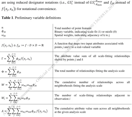
It is necessary to introduce some preliminary definitions, which are presented in Table 1. These are used throughout the remainder of this paper. We define them at this early stage for the sake of readability of our equations. In addition, please note that we

are using reduced designator notations (i.e., 𝐺𝑆_𝑖∗ instead of 𝐺𝑆_𝑖∗_𝑑

𝑚𝑖𝑛

𝑑𝑚𝑎𝑥

and 𝑓_𝑗𝑘 instead of

𝑓(𝑥_𝑗, 𝑥_𝑘)) for notational convenience.

Table 1. Preliminary variable definitions

𝑛 𝜙𝑗𝑘

𝜔𝑗𝑘

Total number of point features

Binary variable, indicating scale fit (1) or misfit (0) Spatial weights, indicating adjacency of k to j

𝑓(𝑥𝑗, 𝑥𝑘) ≙ 𝑓𝑗𝑘∶= 𝑓 ∶ 𝐷 × 𝐷 → ℝ

A function that maps two input attributes associated with points j and k to a real-valued variable

Γ = ∑ ∑ 𝜙𝑗𝑘𝑓(𝑥𝑗, 𝑥𝑘) 𝑗−1

𝑘≠𝑗 𝑛

𝑗

The attribute value sum of all scale-fitting relationships shared by points j and k

Φ = ∑ ∑ 𝜙𝑗𝑘 𝑗−1

𝑘≠𝑗 𝑛

𝑗

The total number of relationships fitting the analysis scale

𝑊 = ∑ ∑ ∑𝜔𝑚𝑗𝜔𝑚𝑘𝜙𝑗𝑘 𝑗−1 𝑘≠𝑗 𝑛 𝑗 𝑛 𝑚

The cumulative number of relationships across all neighborhoods fitting the analysis scale

𝑊𝑖= ∑ ∑𝜔𝑖𝑗𝜔𝑖𝑘𝜙𝑗𝑘 𝑗−1

𝑘≠𝑗 𝑛

𝑗

The number of scale-fitting relationships adjacent to observation i

𝐴 = ∑ ∑ ∑𝜔𝑚𝑗𝜔𝑚𝑘𝜙𝑗𝑘 𝑗−1 𝑘≠𝑗 𝑛 𝑗 𝑛 𝑚

𝑓(𝑥𝑗, 𝑥𝑘)

The cumulative attribute value sum across all neighborhoods at the given analysis scale

The definition of the proposed statistic is based on the original statistic as given by (1). Most formulas in the text are given without derivation. More detailed derivations can be found in appendices 1 to 5. Equation 3 shows our modified version of a scale-sensitive Gi* statistic:

𝐺𝑆𝑖∗ =

∑ ∑𝑗−1𝑘≠𝑗𝜔𝑖𝑗𝜔𝑖𝑘𝜙𝑗𝑘𝑓𝑗𝑘 𝑛

𝑗

∑ ∑ ∑𝑛𝑗 𝑛𝑘 𝑘−1𝑚≠𝑘𝜔𝑗𝑘𝜔𝑗𝑚𝜙𝑘𝑚𝑓𝑘𝑚

As we are operating on pairwise relationships between tuples of observations, the indices j and k represent the two observations being involved in that relationship. Thereby, the indices j and k have to be different. Otherwise, a single point would be set into a relationship to itself. An additional indicator variable denoted ϕjk has also been

included. Its value is 1 if the distance between two contiguous features j and k is within the interval [dmin, dmax], and 0 otherwise. Furthermore, the spatial weights matrix ω is

evaluated twice. This is necessary because both observations j and k must be adjacent to observation i. These modifications allow the inclusion of scale-adjusted neighborhoods as described in Section 4.2 and lead to a match between nominator and denominator scales.

Under the null hypothesis (H0) of spatial independence, each outcome of function f is supposed to be occurring equally likely (i.e., P(fjk) = 1/n). Furthermore, we

suppose pairwise independence between those outcomes. It follows that the expectation for f is estimated by:

𝐸̂[𝑓] = ∑ ∑ 𝜙𝑗𝑘𝑓𝑗𝑘

𝑗−1 𝑘≠𝑗 𝑛 𝑗

Φ (4)

By using (4), we can define the empirical expectation of the GSi*statistic under H0 (equation 5). The first factor and the denominator in (5) are constant across all neighborhoods. Therefore, these can be ignored and the equation reduces to Wi/W. It

follows that the statistic’s local expectation is supposed to be proportional to the respective neighborhood’s fraction among all neighborhoods at the given scale. This is analogous to the original method.

𝐸̂[𝐺𝑆𝑖∗] =

𝐸̂[𝑓] ∙ 𝑊𝑖

𝐴 (5)

∼𝑊𝑖 𝑊

In equations (6) and (7), we develop equations for the variance of the GSi* statistic. Therefore, we first need an equation for the estimate of the expectation of the squared test statistic (6). This is then used to estimate the empirical variance (7) by applying the so called one-pass algorithm (Chan et al. 1983).

𝐸̂[𝐺𝑆𝑖∗2] ₌

𝑊𝑖∑ ∑ 𝜙𝑗𝑘𝑓𝑗𝑘2 𝑗−1 𝑘≠𝑗 𝑛 𝑗

Φ +

𝑊𝑖(𝑊𝑖− 1) (Γ2− ∑ ∑ (𝜙𝑗𝑘𝑓𝑗𝑘) 2 𝑗−1

𝑘≠𝑗 𝑛

𝑗 )

Φ(Φ − 1) 𝐴2

(6)

𝑉𝑎𝑟̂ 𝐺𝑆_𝑖∗

=

𝑊𝑖∑ ∑ 𝜙𝑗𝑘𝑓𝑗𝑘2 𝑗−1 𝑘≠𝑗 𝑛 𝑗

Φ −

𝑊𝑖2Γ2

Φ2 +

2𝑊𝑖(Γ2− ∑ ∑ (𝜙𝑗𝑘𝑓𝑗𝑘) 2 𝑗−1

𝑘≠𝑗 𝑛

𝑗 )

Φ(Φ − 1) 𝐴2

(7)

As expected, the variance under H0 becomes 0 if there are no neighbors in the vicinity of observation i (i.e., Wi = 0). The same applies if no corresponding scale-fitting

zero if the overall neighborhood sum equals zero. In contrast, the variance is greater than zero if all observations are contained in the neighborhood of the current feature. This is a difference from the original method. However, this becomes clear when recalling the statistic’s principle: One neighborhood is compared against all other neighborhoods. Thus, the denominator is always greater than the nominator, resulting in a nonzero variance.

The maximum value of our statistic is reached when all neighborhoods mutually contain each other. In such circumstances, the aggregation of all ϕjk for any tuple across

the whole neighborhood forms an all-ones matrix. It follows that the maximum value of the GSi* statistic is given as:

max 𝐺𝑆𝑖∗ =

1

𝑛 (8)

Accordingly, the minimum value is reached if no values except the investigated observation itself are contained in some neighborhood. It follows that the minimum value is given by:

min 𝐺𝑆𝑖∗ = 0 (9)

Equations (8) and (9) show that the range of the GSi* statistic is not fixed. This is a major difference compared to the original G statistics, which range is the interval [0,1]. In contrast, the GSi* statistic depends on the number of input features. Thus, two GSi* values should not be compared with each other directly. A comparison is only meaningful after standardization. The standardized version of GSi* is given in (10). Applying this equation produces standard deviates (i.e., z-scores), which appear to be on the interval [-∞, ∞]. Furthermore, following the well-known central limit theorem, these scores tend to be approximately normal, given a sufficiently large sample size. Therefore, these scores can be evaluated by means of normal theory.

𝑍𝐺𝑆_𝑖∗ =

∑ ∑ 𝜔𝑖𝑗𝜔𝑖𝑘𝜙𝑗𝑘𝑓𝑗𝑘 𝑗−1

𝑘≠𝑗 𝑛

𝑗 −

∑ ∑ 𝜙𝑗𝑘𝑓𝑗𝑘 𝑗−1 𝑘≠𝑗 𝑛 𝑗

Φ ∙ 𝑊𝑖

√𝑊𝑖∑ ∑ 𝜙𝑗𝑘𝑓𝑗𝑘2 𝑗−1 𝑘≠𝑗 𝑛 𝑗

Φ +

𝑊𝑖(𝑊𝑖− 1) (Γ2− ∑ ∑ (𝜙𝑗𝑘𝑓𝑗𝑘) 2 𝑗−1 𝑘≠𝑗 𝑛

𝑗 )

Φ(Φ − 1) −

𝑊𝑖2(∑ ∑𝑗−1𝑘≠𝑗𝜙𝑗𝑘𝑓𝑗𝑘 𝑛

𝑗 )

2

Φ2

(10)

5. Empirical comparison between 𝑮𝑺_𝒊∗ and 𝑮_𝒊∗

5.1 Dataset description

The datasets we used were extracted from the social media service Twitter. They originate from an urban setting in the city of San Francisco, CA. We used two randomly chosen time slots. One of them covers the time period of January 30, 2014, from 8p.m. until 10p.m.; the second slot covers a whole week from the 20th of January until the 26th of January 2014.

Our automated crawler leveraged the public Twitter Streaming API. Since we are interested in applying methods from spatial statistics, we restricted our query to georeferenced tweets only. We crawled all tweets from a bounding box covering the city of San Francisco and its immediate surroundings. The bounding box had a size of approximately 15x15km. We did not restrict our data collection by using keywords or any other type of filter. The subsets of our dataset that we used for this paper sum up to a size of 1,291 tweets (for the two-hour slot) and 69,345 tweets (for the one-week slot). Figure 2 provides an overview of this subset and shows its distribution over the city.

5.2 Preprocessing and data preparation

The crawled datasets consist of textual tweets. However, our approach as well as the original 𝐺_𝑖∗ statistic are designed for dealing with numerical values. Thus, we first have to transform the textual tweets into some numerical representation. We have chosen to use similarities among the tweets for our test and comparative study. In a realistic scenario, high similarity scores might be interpreted as indicators of coherent social activity (i.e., people might be reporting about similar topics). In order to obtain meaningful similarities, several steps are conducted.

The first step is to split up the cohesive strings of words into single tokens. The tokenization process that we used follows some rules that have been adapted from the recent literature: The texts are split up at case changes, except if they occur at the beginning of a word (Metke-Jimenez et al. 2011); Twitter’s specific symbols (e.g., #, @) are kept (O’Connor et al. 2010), and short forms or contractions of English words (e.g., I’m) are retained (Pak & Paroubek 2010). Moreover, we split the tweets at whitespaces and punctuation marks. A large portion of the resulting tokens occurs frequently, but adds little meaning (e.g., “to”, “or”). Therefore, these so-called stop words are removed from the corpus in the second step. For this purpose, we relied on the English stop word list provided by the database system PostgreSQL.

The actual similarity assessment is based on the method of Latent Semantic Indexing (LSI) (Deerwester et al. 1990). The core principle of this method is based on a singular value decomposition (SVD). First of all, the tokens are transformed into normalized frequencies (called Term Frequency – Inverse Document Frequency (TF-IDF) scores). These are then used for extracting inherent components, based on word co-occurrence. LSI works in an unsupervised manner. Thus, no a priori knowledge about the text corpus is needed. However, a criterion for maintaining a reasonable number of components is required. In our experiments, we used a broken stick model for this purpose. This approach is usually used for modeling resource allocation in ecology. However, it has also proven to be useful for application of the SVD (Cangelosi & Goriely 2007).

Again, note that our approach for assessing similarities has been chosen for the sake of producing numerical tweet representations. Neither similarity assessment itself nor analyzing our test site is the focus of this paper. Thus, the chosen approach is appropriate for our experiments regarding the proposed statistic. We point out that more accurate semantic similarity approaches might be available (e.g., Latent Dirichlet Allocation (Blei et al. 2003) or probabilistic LSI (Hofmann 1999)). However, these are more sophisticated and require more detailed a priori knowledge about the composition of the text corpus. Whenever realistic conclusions are to be drawn from any dataset, careful consideration should be given to the choice of an appropriate semantic similarity approach.

5.3 Comparison between GSi* and Gi*

Section 4.1. Moreover, we also demonstrate that these issues are solved by our proposed solution.

Overemphasis of dominant scales

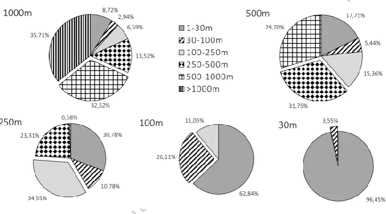
Recall the property of scale mixing within social media data. Figure 3 illustrates the average composition of five differently scaled neighborhoods. These neighborhoods are heterogeneous. In most cases, the actual scale of interest contributes only approximately 30% of the total attribute value sum. This means that approximately 70% of all variation is contributed by scales other than the one of interest. Accordingly, when applying standard (i.e., single-scale) approaches for neighborhood definition, all these scales are considered together.

Figure 3. Average composition of the attribute value sum for five classes of

neighbourhood sizes. The respective scales of interest are highlighted by displacement. Dataset: Twitter, 30th of January 2014, 8pm until 10pm.

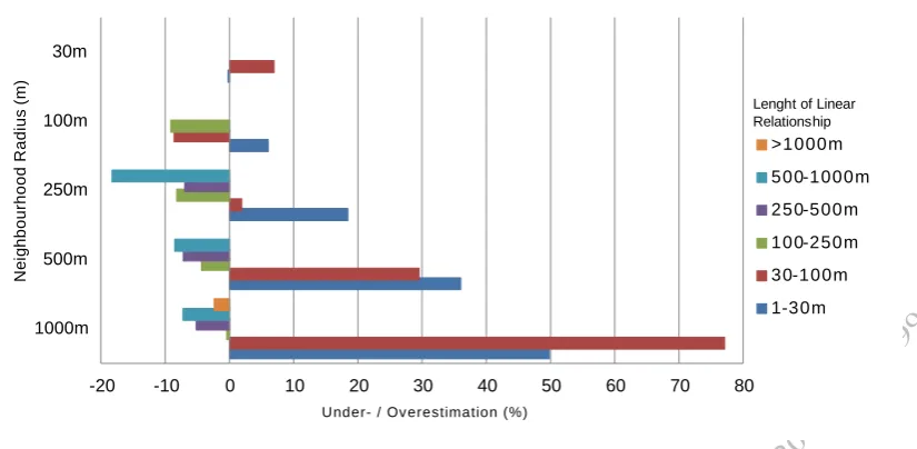
Figure 4. Under- / overestimation of various scales within neighbourhoods at different analysis scales. Dataset: Twitter, 30th of January 2014, 8pm until 10pm.

The problems described above affect the original Gi* statistic in two ways: On the one hand, scales are superimposed in the focal neighborhoods. On the other hand, these are then compared against an overall mixture of scales (i.e., the denominator of the statistic). The larger the scale, the more different scales are potentially being mixed up. Figure 5 shows one of the effects caused by that behavior. The mean of the z-values obtained through the Gi* statistic shows a strong trend with increasing scale. However, we are dealing with a standardized version of the statistic. Following the central limit theorem, the resulting standard variates are expected to be approximately normal. Thus, the mean is expected to be an unbiased estimator of the expectation, which should be close to zero in the present case. That is obviously not true for Gi* when it is applied to social media datasets. It is very likely that this effect is caused by the scale mixture described in the previous paragraph. That mixture implies different underlying populations, since different phenomena might be operating at the different scales. Thus, there are also different means present in the mixture. The mean of the z-values is influenced by that variety of means, which in turn leads to the observed bias.

Figure 5. Arithmetic means of Z(Gi*) and Z(GSi*) across all tested scales. Dataset: Twitter, 20th of January until 26th of January.

-20 -10 0 10 20 30 40 50 60 70 80

1000m 500m 250m 100m 30m

Under- / Overestimation (%)

N e ig h b o u rh o o d R a d iu s ( m ) >1000m 500-1000m 250-500m 100-250m 30-100m 1-30m

Lenght of Linear Relationship

Under- / Ov erestimation (%)

0.452

0.579

0.657

0.746

0.904

-0.002 0.003 0.024 0.034 0.007

-0.1 0.1 0.3 0.5 0.7 0.9

1-30 30-100 100-250 250-500 500-1000

These effects are diminished with our suggested scale-sensitive approach. Our method only extracts those scales from the vicinity of observations that are relevant for the current analysis scale. Thus, each diagram shown in Figure 3 would only consist of one pie slice, each representing the respective scale of interest. The composition of the attribute value sum of the neighborhoods is completely made up of observations fitting the scale of interest. Moreover, the same applies to the comparative size. The modified statistic only includes those observations in any calculation that are fitting the current scale of interest. Therefore, the estimated means obtained through our modified statistic (see Figure 5) remain close to zero across all investigated scales.

Type I/Type II errors

The problem of overemphasizing dominant scales leads to another closely related problem, which is the occurrence of type I/II errors. This is a well-known general issue of all local statistics (Nelson 2012). It is usually caused by missing strategies for facing multiple testing problems. However, when dealing with multi-scale datasets, this problem is further exacerbated by an additional problem. When some scales are dominating a dataset, they also hide weaker phenomena at less dominant scales. However, these less pronounced phenomena are not necessarily less important. Some analyst might indeed be interested in analyzing these weaker phenomena. Now, several different configurations are possible: Some weaker phenomenon might, for instance, consist of some high-value accumulation. These values might, however, only be high according to their own respective scale. Some contiguous and more dominant scale might comprise even higher values. In such situations, the dominance of the other scale with high values leads to type II errors. H1 is rejected although high values are present at the adjusted scale of interest. These values just appear to be quite low in comparison to the more dominant adjacent scale that is present in the same neighborhood. The same situation occurs if a phenomenon of interest shows low-value accumulation. Higher values at another scale are again artificially raising the neighborhood score, leading to H1 rejection. In contrast, type I errors occur whenever a scale of interest is actually not out of the ordinary, but gets interfered by a more dominant scale. This situation might occur in both directions, either toward low values (cold spots) or high values (hot spots). In such cases, the neighborhood score is artificially raised (or lowered) to a level that leads to a wrong acceptance of H1.

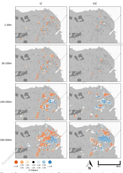
comparison, the results obtained through our modified approach show a considerably lower number of extraordinary observations. Since the dominance of scales is not affecting the results, that method only evaluates 3.77% of the tweets to be somehow abnormal. Another issue that can be seen in Figure 6 is the existence of type I errors. Because of the dominance effect described above, H0 is rejected too often. This does not only appear at the dominant scales, but is transferred onto all larger levels as well. Hot or cold spots occurring at small scales appear to be acting like “seeds” that are being enlarged at the next larger scale. Thus, the type I errors can be found with increasing frequency by enlarging the analysis scale. This effect also does not occur in the results obtained through our proposed statistic. Every scale is only analyzed against observations at the same scale. Thus, there is no dominance to be transferred, resulting into a lower number of type I errors. However, the effect of “seed” locations with Gi* leads to another issue that is described in the following subsection.

Loss of statistical independence between scales

We already mentioned the spill-over effect of dominant scales that are transferred onto all larger ones. We can also observe that this effect results into “seed” locations that appear to be growing as the scale is getting enlarged. However, this phenomenon leads to another much more serious problem, which is the loss of independence between spatial autocorrelation results obtained for different scales. We assume all possible outcomes of spatial autocorrelation statistics to be equally likely. That is, we assume the probabilities to be P(xa) = ∑ xa/n. If different scales are being admixed, however, this

assumption is no longer verified; this occurs, for instance, when assessing a non-zero spatial autocorrelation at some small scale. If the scale is adjusted to some larger value, these small-scale instances are again included. The problem is that now, the outcome of zero has become impossible. The effect of the non-zero spatial autocorrelation at the smaller scale might be blurred (due to mixing) or be changed in nature (from negative to positive or vice versa) because other observations are included in the neighborhood. However, the result of having no autocorrelation is no longer possible at any larger scale. In other words, the independence requirement P(xb|xa) = P(xb) is no longer met.

Figure 6. Two series of analysis results. The left-hand side was obtained by applying the original Gi*statistic, the right-hand side originates from our proposed GSi*statistic; Dataset: Twitter, 30th of January 2014, 8pm until 10pm; Base data: VMAP, National Geospatial-Intelligence Agency, US.

Gi* GSi*

1-30m

30-100m

100-250m

250-500m

0 4km

>2.58 1.96 -2.58

1.65

-1.96 <-2.58

-2.58 --1.96 -1.96

--1.65 -1.65

-1.65

6. Conclusions

The arising interest in analyzing social media feeds and other kinds of human-generated datasets compels us to address the specific problems of such data. One of those problems is their multi-scale nature that is due to the uncontrolled data acquisition process. However, most spatial statistics are designed for single-scale datasets that result from controlled experiments. This paper introduced a scale-sensitive version of the popular Gi* statistic. The proposed approach comprises an alternative approach for neighborhood definition and a scale-adjustment of the statistic itself. Moreover, some scale-related issues that arise when dealing with multi-scale datasets are highlighted by comparing the results obtain through the original and the proposed statistics. These comparisons are carried out on a Twitter dataset for the city of San Francisco, CA. The results demonstrate that the suggested approach is better suited for dealing with multi-scale datasets, because it allows analyzing certain multi-scales without cross-multi-scale interferences. Thus, it can be used in real-world scenarios whenever social media or other human-generated datasets are analyzed.

However, scale-related effects affecting social media datasets are not yet fully understood. The list of issues mentioned in Section 5 is given without claiming completeness. There might be many more effects that are still to be discovered. Moreover, the effects we listed and observed have not yet been fully investigated. Thus, future research should focus on getting a better understanding of the multi-scale nature of user-generated datasets. In addition, there are many more methods from spatial statistics and other fields that are not yet sufficiently capable of dealing with multi-scale datasets. Our suggested approach might serve as a starting point for initiating methodological research towards multi-scale enablement.

With respect to local autocorrelation statistics in general, more emphasis should be put on the definition of the null hypothesis. Geographic space imposes uncontrolled variance, due to varying local environmental conditions (Goodchild 2009, Anselin 1989). Local statistics such as Gi* and our proposed solution already account for heterogeneity with respect to the spatial distribution of observations. In contrast, they usually include constant expectations of the observed variable. However, the outcomes of those variables might also be influenced by nonstationary environmental conditions. One way of overcoming this problem might be to use location-dependent expectation functions instead of constant values. Corresponding local values might be determined by methods such as Geographically Weighted Regression (Brunsdon et al. 1996). However, a specific problem to social media data is that the underlying driving forces are not yet fully understood.

Acknowledgements:

substantive contributions and for his help in creating appealing maps. We also thank Shih-Pei Chen (Max Planck Institute for the History of Science, Berlin) for proof-reading this article. Furthermore, this work has partially been funded by the Klaus Tschira Stiftung gGmbH as well as by the Graduate Funding Programme of the state of Baden-Württemberg.

References

Aldstadt, J., and Getis, A., 2006. Using AMOEBA to Create a Spatial Weights Matrix and Identify Spatial Clusters. Geographical Analysis, 38, 327 – 343.

Allen, T.F.H., and Hoekstra, T.W., 1992. Toward a Unified Ecology. New York: Columbia University Press.

Anselin, L., 1989. What is Special about Spatial Data? Alternative Perspectives on Spatial Data Analysis. Technical Report. National Centre for Geographic Information and Analysis, Santa Barbara, CA.

Anselin, L., 1995. Local Indicators of Spatial Association – LISA. Geographical Analysis, 27 (2), 93 – 115.

Blei, D.M., Ng, A.Y., and Jordan, M.I., 2003. Latent Dirichlet Allocation. The Journal of Machine Learning Research, 3, 993 – 1022.

Boots, B., 2003. Developing Local Measures of Spatial Association for Categorical Data. Journal of Geographical Systems, 5, 139 – 160.

Brunsdon, C., Fotheringham, AS., and Charlton, M., 1996. Geographically Weighted Regression: A Method for Exploring Spatial Non-Stationarity. Geographical Analysis, 28 (4), 281 – 298.

Cangelosi, R., and Goriely, A., 2007. Component Retention in Principal Component Analysis with Application to cDNA Microarray Data. Biology Direct, 2 (2). Chan, T.F., Golub, G.H., and Randall, J.L., 1983. Algorithms for Computing the

Sample Variance: Analysis and Recommendations. The American Statistician, 37 (3), 242 – 247.

Cliff, A.D., and Ord., J.K., 1969. The Problem of Spatial Autocorrelation. In: Scott, A. J. (ed.) London Papers in Regional Science (1), Studies in Regional Science. London: Pion, 25 – 55.

Crooks, A., Croitoru, A., Stefanidis, A., and Radzikowski, J., 2013. #Earthquake: Twitter as a Distributed Sensor System. Transactions in GIS, 17 (1), 124 – 147. Dacey, M.F., 1965. A Review on Measures of Contiguity for Two and k-Color Maps.

Technical Report No. 2, Spatial Diffusion Study. Department of Geography, Northwestern University, Evanston.

Deerwester, S., Dumais, S.T., Furnas, G.W., Landauer, T.K., and Harshman, R., 1990. Indexing by Latent Semantic Analysis. Journal of the American Society for Information Science, 41 (6), 391 – 407.

Fotheringham, A.S., 2009. “The Problem of Spatial Autocorrelation” and Local Spatial Statistics. Geographical Analysis, 41, 398 – 403.

Geary, R.C., 1954. The Contiguity Ratio and Statistical Mapping. The Incorporated Statistician, 5 (3), 115 – 146.

Getis, A., 2006. Spatial Statistics. In: Longley, P.A., Goodchild. M.F., Maguire, D.J., and Rhind, D.W. (eds.) Geographical Information Systems: Principles, Techniques, Management and Applications. Hoboken, NJ: Wiley & Sons, 239 – 251.

Getis, A., 2009. Spatial Weights Matrices. Geographical Analysis, 41, 404 – 410. Getis, A., 2010. Spatial Autocorrelation. In: Fischer, M., and Getis, A. (eds.) Handbook

of Applied Spatial Analysis. Berlin: Springer, 255 – 278.

Getis, A., and Ord, J.K., 1992. The Analysis of Spatial Association by Use of Distance Statistics. Geographical Analysis, 24 (3), 189 – 206.

Getis, A., and Aldstadt, J., 2004. Constructing the Spatial Weights Matrix Using a Local Statistic. Geographical Analysis, 36 (2), 90 – 104.

Gibson, C.C., Ostrom, E., and Ahn, T.K., 2000. The Concept of Scale and the Human Dimensions of Global Change: A Survey. Ecological Economics, 32, 217 – 239. Goodchild, M., 2001. Models of Scale and Scales of Modelling. In: Tate, N.J. and

Atkinson, P.M. (eds) Modelling Scale in Geographical Information Science. Chichester: John Wiley & Sons, 3 – 10.

Goodchild, M., 2009. What Problem? Spatial Autocorrelation and Geographic Information Science. Geographical Analysis, 41, 411 – 417.

Hawelka, B., Sitko, I., Beinat, E., Sobolevsky, S., Kazakopoulos, P., and Ratti, C., 2014. Geo-located Twitter as Proxy for Global Mobility Patterns. Cartography and Geographic Information Science, 41 (3), 260 – 271.

Hofmann, T., 1999. Probabilistic Latent Semantic Indexing. In: Gey, F., Hearst, M., and Tong, R. (eds.) Proceedings of the 22nd annual international ACM SIGIR conference on research and development in information retrieval, 50 – 57. Lam, N.S.-N., and Quattrochi, D.A., 1992. On the Issues of Scale, Resolution, and

Fractal Analysis in the Mapping Sciences. The Professional Geographer, 44(1), 88 – 98.

Leibovici, D.G., Claramunt, C., Le Guyader, D., and Brosset, D., 2014. Local and Global Spatio-Temporal Entropy Indices Based on Distance-Ratios and Co-Occurrences Distributions. International Journal of Geographical Information Science, 28 (5), 1061 – 1084.

LeSage, J.P., 2003. A Family of Geographically Weighted Regression Models. In: Anselin, L., Florax, J.G.M., and Rey, S.J. (eds.) Advances in Spatial Econometrics: Methodology, Tools and Applications. Heidelberg: Springer, 241 – 264.

Lloyd, C., 2011. Local Models for Spatial Analysis. London: Taylor & Francis.

Metke-Jimenez, A., Raymond, K., and MacColl, I., 2011. Information Extraction from Web Services: A Comparison of Tokenisation Algorithms. In: Proceedings of the International Workshop on Software Knowledge (SKY 2011). Paris: SciTePress, 12 – 23.

Mitchell, L., Frank, M.R., Harris, K.D., Dodds, P.S., and Danforth, C.M., 2013. The Geography of Happiness: Connecting Twitter Sentiment and Expression, Demographics, and Objective Characteristics of Place. PLoS ONE, 8 (5), doi:10.1371/journal.pone.0064417.

Montello, D.R., 2001. Scale in Geography. In: Smelser, N.J., and Baltes, P.B. (eds.) International Encyclopedia of the Social & Behavioural Sciences. Oxford: Pergamon Press, 13501 – 13504.

Moran, P.A.P., 1950. Notes on Continuous Stochastic Phenomena. Biometrika, 37 (1-2), 17 – 23.

Nelson, T.A., 2012. Trends in Spatial Statistics. The Professional Geographer, 64 (1), 83 – 94.

O’Connor, B., Krieger, M., and Ahn, D., 2010. TweetMotif: Exploratory Search and Topic Summarization for Twitter. In: Hearst, M. (ed.) Proceedings of the Fourth International AAAI Conference on Weblogs and Social Media. Menlo Park: The AAAI Press, 384 – 385.

Ord, J.K., and Getis, A., 1995. Local Spatial Autocorrelation Statistics: Distributional Issues and an Application. Geographical Analysis, 27 (4), 286 – 306.

Ord, J.K., and Getis, A., 2001. Testing for Local Spatial Autocorrelation in the Presence of Global Autocorrelation. Journal of Regional Science, 41 (3), 411 – 432. Pak, A., and Paroubek, P., 2010. Twitter as a Corpus for Sentiment Analysis and

Opinion Mining. In: Calzolari, N., and Choukri, K. (eds.) Proceedings of the Seventh International Conference on Language Resources and Evaluation (LREC’10). Paris: European Language Resources Association, 1320 – 1326. Rogerson, P.A., 1998. The Detection of Clusters Using a Spatial Version of the

Chi-Square Goodness-of-Fit Statistic. Geographical Analysis, 31 (1), 130 – 147. Rogerson, P.A., and Kedron, P., 2012. Optimal Weights for Focused Tests of Clustering

Using the Local Moran Statistic. Geographical Analysis, 44, 121 – 133.

Ruiz, M., López, F., and Páez, A., 2010. Testing for Spatial Association of Qualitative Data Using Symbolic Dynamics. Journal of Geographical Systems, 12, 281 – 309.

Smelser, N.J., 1995. Problematics of Sociology. Berkeley: University of California Press.

Tango, T., 1995. A Class of Tests for Detecting ‘General’ and ‘Focused’ Clustering of Rare Diseases. Statistics in Medicine, 14, 2323 – 2334.

Tobler, W.R., 1988. Resolution, Resampling, and all that. In: Mounsey, H., and Tomlinson, R. (eds.) Building Database for Global Science. London: Taylor & Francis, 129 – 137.

Zhang, T., and Lin, G., 2006. A Supplemental Indicator of High-Value or Low-Value Spatial Clustering. Geographical Analysis, 38, 209 – 225.

Zhang, T., and Lin, G., 2007. A Decomposition of Moran’s I for Clustering Detection. Computational Statistics & Data Analysis, 51, 6123 – 6137.

Zipf, G.K., 1949. Human Behaviour and the Principle of Least Effort. Cambridge, MA: Addison-Wesley.

Appendix 1: Derivation of the Empirical Expectation of GSi*

𝐸̂[𝐺𝑆𝑖∗] ₌ ∑ ∑ 𝜔𝑖𝑗𝜔𝑖𝑘𝜙𝑗𝑘𝐸̂[𝑓] 𝑗−1

𝑘≠𝑗 𝑛 𝑗

∑ ∑ ∑𝑛𝑗 𝑛𝑘 𝑘−1𝑚≠𝑘𝜔𝑗𝑘𝜔𝑗𝑚𝜙𝑘𝑚𝑓𝑘𝑚

(11)

= 𝐸̂[𝑓] ∑ ∑ 𝜔𝑖𝑗𝜔𝑖𝑘𝜙𝑗𝑘

𝑗−1 𝑘≠𝑗 𝑛 𝑗

∑ ∑ ∑𝑛𝑗 𝑛𝑘 𝑘−1𝑚 𝜔𝑗𝑘𝜔𝑗𝑚𝜙𝑘𝑚𝑓𝑘𝑚

= 𝐸̂[𝑓] ∙ 𝑊𝑖 𝐴

Since Ê[f] and A are constant, we can infer that the expectation is proportional to the share of the neighbourhood’s size among the overall sum of relationship outcomes:

∼𝑊𝑖 W

Appendix 2: Derivation of the Expectation of the Squared GS Statistic

𝐺𝑆𝑖∗2 =

∑ ∑ ∑ ∑𝑛𝑚 𝑝≠𝑚𝑚−1𝜔𝑖𝑗𝜔𝑖𝑘𝜔𝑖𝑚𝜔𝑖𝑝𝜙𝑗𝑘𝜙𝑚𝑝𝑓𝑗𝑘𝑓𝑚𝑝 𝑗−1

𝑘≠𝑗 𝑛 𝑗

∑ ∑ ∑ ∑ ∑ ∑ 𝜔𝑗𝑘𝜔𝑗𝑚𝜔𝑝𝑞𝜔𝑝𝑠𝜙𝑘𝑚𝜙𝑞𝑠𝑓𝑘𝑚𝑓𝑞𝑠 𝑞−1 𝑠≠𝑞 𝑛 𝑞 𝑛 𝑝 𝑘−1 𝑚≠𝑘 𝑛 𝑘 𝑛 𝑗 (12)

𝐸̂[𝑓1, 𝑓2] =

∑ ∑𝑗−1𝑘≠𝑗∑ ∑𝑛𝑚 𝑚−1𝑝≠𝑚𝜙𝑗𝑘𝑓𝑗𝑘𝜙𝑚𝑝𝑓𝑚𝑝 𝑛

𝑗 − ∑ ∑ (𝜙𝑗𝑘𝑓𝑗𝑘)

2 𝑗−1

𝑘≠𝑗 𝑛 𝑗

Φ(Φ − 1) (13)

=Γ

2_{− (∑ ∑ (𝜙} 𝑗𝑘𝑓𝑗𝑘)

2 𝑗−1

𝑘≠𝑗 𝑛

𝑗 )

Φ(Φ − 1)

𝐸̂[𝑓2_{] =} ∑ ∑ 𝜙𝑗𝑘𝑓𝑗𝑘 2 𝑗−1 𝑘≠𝑗 𝑛 𝑗 Φ (14)

Solving (12) leads to quadratic and non-quadratic terms. Thus, we need Ê[f²] and Ê[f1,f2]

for inferring the expectation of the squared GS statistic. Both of these values are constant. Therefore, we can extract them from the sums. Furthermore, ω and ϕ are binary and ω²ij=𝜔, 𝜙²jk = 𝜙jk. Accordingly we can write:

𝐸̂[𝐺𝑆𝑖∗2] =

𝑊𝑖∙ 𝐸[𝑓2] + 𝑊𝑖(𝑊𝑖− 1) ∙ 𝐸̂[𝑓1, 𝑓2]

𝐴2 (15)

=

𝑊𝑖∑ ∑ 𝜙𝑗𝑘𝑓𝑗𝑘2 𝑗−1 𝑘≠𝑗 𝑛 𝑗

Φ +

𝑊𝑖(𝑊𝑖− 1) (Γ2− ∑ ∑ (𝜙𝑗𝑘𝑓𝑗𝑘) 2 𝑗−1

𝑘≠𝑗 𝑛

𝑗 )

Appendix 3: Derivation of the Empirical Variance of the Local GSi* Statistic

Applying the Steiner translation theorem leads to the variance of the statistic:

𝑉𝑎𝑟̂ _𝐺𝑆

𝑖∗ = 𝐸̂[𝐺𝑆𝑖∗2] − (𝐸̂[𝐺𝑆𝑖∗]) 2

(16)

=

𝑊𝑖∑ ∑𝑛𝑗 𝑗−1𝑘≠𝑗𝜙𝑗𝑘𝑓𝑗𝑘2

Φ +

𝑊𝑖(𝑊𝑖− 1) (Γ2− ∑ ∑ (𝜙𝑗𝑘𝑓𝑗𝑘) 2 𝑗−1

𝑘≠𝑗 𝑛

𝑗 )

Φ(Φ − 1) −

𝑊𝑖2(∑ ∑𝑛𝑗 𝑗−1𝑘≠𝑗𝜙𝑗𝑘𝑓𝑗𝑘) 2

Φ2

𝐴2

Appendix 4: Derivation of the maximum of the GSi* Statistic

max 𝐺𝑆𝑖∗ =

∑ ∑𝑛𝑗 𝑛𝑘=𝑗+1𝜔𝑖𝑗𝜔𝑖𝑘𝜙𝑗𝑘𝑓𝑗𝑘

𝑁 ∙ ∑ ∑𝑛𝑗 𝑛𝑘=𝑗+1𝜔𝑖𝑗𝜔𝑖𝑘𝜙𝑗𝑘𝑓𝑗𝑘

(17)

= ∑ ∑ 𝜔𝑖𝑗𝜔𝑖𝑘𝑓𝑗𝑘

𝑛 𝑘=𝑗+1 𝑛 𝑗

𝑛 ∙ ∑ ∑𝑛𝑗 𝑛𝑘=𝑗+1𝜔𝑖𝑗𝜔𝑖𝑘𝑓𝑗𝑘

= 1 𝑛

Appendix 5: Derivation of the Standardised GSi* Statistic

𝑍𝐺𝑆_𝑖∗

= 𝐺𝑆𝑖 ∗_{− 𝐸̂[𝐺𝑆}

𝑖∗]

√𝑉𝑎𝑟̂𝐺𝑆𝑖∗

(18)

=

∑ ∑𝑛𝑗 𝑗−1𝑘≠𝑗𝜔𝑖𝑗𝜔𝑖𝑘𝜙𝑗𝑘𝑓𝑗𝑘−

∑ ∑ 𝜙𝑗𝑘𝑓𝑗𝑘 𝑗−1 𝑘≠𝑗 𝑛 𝑗

Φ ∙ 𝑊𝑖

𝐴

√(𝑊𝑖∑ ∑ 𝜙𝑗𝑘𝑓𝑗𝑘 2 𝑗−1 𝑘≠𝑗 𝑛 𝑗 Φ +

𝑊𝑖(𝑊𝑖− 1) (Γ2− ∑ ∑ (𝜙𝑗𝑘𝑓𝑗𝑘) 2 𝑗−1 𝑘≠𝑗 𝑛

𝑗 )

Φ(Φ − 1) −

𝑊_𝑖2_{(∑ ∑ 𝜙}

𝑗𝑘𝑓𝑗𝑘

𝑗−1 𝑘≠𝑗 𝑛 𝑗 ) 2 Φ2 𝐴2 ) =

∑ ∑ 𝜔𝑖𝑗𝜔𝑖𝑘𝜙𝑗𝑘𝑓𝑗𝑘 𝑗−1

𝑘≠𝑗 𝑛

𝑗 −

∑ ∑ 𝜙𝑗𝑘𝑓𝑗𝑘 𝑗−1 𝑘≠𝑗 𝑛 𝑗

Φ ∙ 𝑊𝑖

𝐴

√𝑊𝑖∑ ∑ 𝜙𝑗𝑘𝑓𝑗𝑘2 𝑗−1 𝑘≠𝑗 𝑛 𝑗

Φ +

𝑊𝑖(𝑊𝑖− 1) (Γ2− ∑ ∑ (𝜙𝑗𝑘𝑓𝑗𝑘) 2 𝑗−1 𝑘≠𝑗 𝑛

𝑗 )

Φ(Φ − 1) −

𝑊𝑖2(∑ ∑ 𝜙𝑗𝑘𝑓𝑗𝑘 𝑗−1 𝑘≠𝑗 𝑛 𝑗 ) 2 Φ2 𝐴

= ∑ ∑ 𝜔𝑖𝑗𝜔𝑖𝑘𝜙𝑗𝑘𝑓𝑗𝑘

𝑗−1 𝑘≠𝑗 𝑛

𝑗 −

∑ ∑ 𝜙𝑗𝑘𝑓𝑗𝑘 𝑗−1 𝑘≠𝑗 𝑛 𝑗

Φ ∙ 𝑊𝑖

√𝑊𝑖∑ ∑ 𝜙𝑗𝑘𝑓𝑗𝑘2 𝑗−1 𝑘≠𝑗 𝑛 𝑗

Φ +

𝑊𝑖(𝑊𝑖− 1) (Γ2− ∑ ∑ (𝜙𝑗𝑘𝑓𝑗𝑘) 2 𝑗−1 𝑘≠𝑗 𝑛

𝑗 )

Φ(Φ − 1) −

𝑊𝑖2(∑ ∑𝑗−1𝑘≠𝑗𝜙𝑗𝑘𝑓𝑗𝑘 𝑛

𝑗 )

2