Cheryl Victoria Wood
A Thesis Submitted for the Degree of
at the
University of St Andrews
2014
Full metadata for this item is available in
St Andrews Research Repository
at:
http://research-repository.st-andrews.ac.uk/
Please use this identifier to cite or link to this item:
http://hdl.handle.net/10023/6389
This item is protected by original copyright
Validating A Calcium Tracer Based
Tree-Ring Dating Method For
Tropical Wood
Cheryl Victoria Wood
A thesis submitted to the University of St Andrews for the degree of Doctor of Philosophy
Department of Earth and Environmental Sciences
School of Geography and Geosciences
i
I, Cheryl Wood, hereby certify that this thesis, which is approximately 63,500 words in length,
has been written by me, that it is the record of work carried out by me or principally by myself
in collaboration with others as acknowledged, and that it has not been submitted in any
previous application for a higher degree.
I was admitted as a research student in October, 2007 and as a candidate for the degree of
PhD in October, 2008; the higher study for which this is a record was carried out in the
University of St Andrews between 2007 and 2012.
Date Signature of candidate
I hereby certify that the candidate has fulfilled the conditions of the Resolution and
Regulations appropriate for the degree of PhD in the University of St Andrews and that the
candidate is qualified to submit this thesis in application for that degree.
ii
University Library for the time being in force, subject to any copyright vested in the work not
being affected thereby. I also understand that the title and the abstract will be published, and
that a copy of the work may be made and supplied to any bona fide library or research worker,
that my thesis will be electronically accessible for personal or research use unless exempt by
award of an embargo as requested below, and that the library has the right to migrate my
thesis into new electronic forms as required to ensure continued access to the thesis. I have
obtained any third-party copyright permissions that may be required in order to allow such
access and migration, or have requested the appropriate embargo below.
The following is an agreed request by candidate and supervisor regarding the publication of
this thesis:
Embargo on all of print copy for a period of 2 years on the following ground(s):
Publication would preclude future publication
Embargo on all of electronic copy for a period of 2 years on the following ground(s):
Publication would preclude future publication
Date Signature of candidate
iii
The tropics are a key part of the global biosphere. Specifically, the woodland environments
not only moderate large scale climate dynamics, but are also crucial in the global carbon cycle.
Despite this, tropical dendrochronological studies are rare due to the uncertainty in annual
dating from the minimal seasonality in most tropic environments. Without distinct annual tree
rings, dendrochronological dating methods do not work, therefore other dating methods are
required before long term forest growth analyses can be made. Alternatives such as
radiocarbon and stable isotope measurements can be expensive and require high resolution
measurement in order to identify seasonality. This thesis introduces a novel dating method for
tropical trees using calcium as a tracer of annual wood formation. Laser Ablation-ICP-MS
provides a fast, high resolution method for measuring mineral elements which could
potentially provide a solution to the dating of tropical trees.
Initially, Scots pine provided an excellent testing species for the development of both the
methodological and analytical dating methods proposed through this thesis. It’s well defined,
annually dated ring structure formed the basis of seasonal signal detection and the
development of an objective analysis for dating. This was achieved by the continuous
measurement of calcium, and utilising a threshold detection approach to define annual growth
cycles with respect to extreme peaks in the tracer data-series.
The initial success of the calcium dating method using pine allowed for testing the technique
on a tropical trees species from Cameroon which lacks distinct rings. Along with radiocarbon
dating, the robustness of the calcium dating method for this tropical species was assessed.
Promising results were initially found however, these could not be replicated and validation of
this method proved problematic.
Finally, radiocarbon dates were used to assess the nature of the oxygen and carbon stable
isotopic series from the single tree of the same species from the tropical calcium tests. Results
showed that despite the clear cyclic signal present in the oxygen isotope record, this did not
represent an annual signal. These results reinforce the problems associated with tropical
iv
I would like to thank my supervisor, Rob Wilson, for his endless enthusiasm, support and
encouragement throughout this project, and for always making time to discuss things
regardless of how many other students, lectures, proposals or papers he is trying to shuffle at
the time. Thanks should also go to SAGES and the University of St Andrews for their financial
support as well as the TROBIT group for the organisation and financing of the Cameroon field
work. I also thank Yit Arn Teh for support with lab costs.
Thanks to Angus Calder for his help in the lab with useful advice and ideas, for his expertise in
maintaining the all of the analytical equipment, and most importantly for the coffee breaks!
Thanks must also to Nora Hanson, Gustavo Saiz and Chris Wurster for all their help and advice
both in and out of the lab.
I would like to thank Georgina King for all the support she has provided since we met at the
start of our postgraduate careers, Amy Tavendale for her continued support and always being
there at beer o’clock, and Joanna Fraser for the much needed lunch and cake relief!
Last but not least, thanks to my family for their support, and especially to Dean who has
encouraged and supported me throughout, and in particular for his understanding in the last
few write-up months when I can only imagine that I was not the most pleasant person to live
v
Declaration ... i
Abstract ... iii
Acknowledgements ...iv
Table of Contents ... v
Table of Figures ... ix
List of Tables ... xvi
Chapter 1: Introduction and Literature Review ... 1
1.1. Project Rationale ... 1
1.2. Dendrochronology ... 3
1.3. Dendrochronology in the Tropics ... 6
1.3.1. Measuring Growth Rates in Tropical Trees ... 11
1.4. Dendrochemistry ... 12
1.4.1. Stable Isotopes in Tree-Rings ... 13
1.4.2. Stable Isotopes in Temperate Trees ... 17
1.4.3. Stable Isotopes in Tropical Trees... 18
1.4.4. Mineral Nutrition in Trees ... 21
1.4.5. Calcium in Trees ... 34
1.4.6. Applications of Mineral Element Dendrochemistry ... 39
1.4.7. Mineral Elements in Tropical Trees ... 40
1.5. Summary ... 42
1.5.1. Thesis Structure ... 44
1.5.2. Aims and Objectives ... 45
Chapter 2: Calcium Tracers and the Dating of Scots Pine ... 46
2.1. Introduction ... 46
2.1.1. Mineral Element Measurement ... 47
2.2. Study Area and Sample Description ... 49
2.3. Materials and Methods ... 50
2.3.1. Sample Preparation ... 50
2.3.2. LA-ICP-MS ... 51
vi
2.3.6. Ring Width Measurements ... 75
2.3.7. Splicing Datasets ... 76
2.3.8. Method for Ring Detection: Threshold Approach ... 80
2.4. Results ... 81
2.4.1. Seasonal Calcium Pattern ... 81
2.4.2. Ring Identification (Threshold Approach) ... 83
2.5. Discussion ... 87
2.5.1. Calcium Seasonality ... 87
2.5.2. Standard Reference Materials... 90
2.5.3. Decreasing Ca signal and Machine Drift ... 91
2.5.4. Data Adjustments ... 92
2.6. Refinement of Methods ... 96
2.6.1. Sample preparation methods ... 96
2.6.2. Standards Reference Materials ... 96
2.6.3. LA-ICP-MS equipment and settings ... 97
2.6.4. Number of replicate tracks... 98
2.7. Future Work ... 98
2.7.1. Spots vs. Tracks ... 99
2.8. Conclusions ... 99
Chapter 3: Calcium Tracers and the Dating of Tropical Trees ... 101
3.1. Introduction ... 101
3.2. Study Area and Sample Collection ... 102
3.2.1. Preliminary Radiocarbon Age ... 106
3.3. Materials and Methods ... 108
3.3.1. Sample Preparation ... 108
3.3.2. LA-ICP-MS ... 110
3.3.3. Data Adjustments ... 112
3.3.4. Calcium Dating ... 113
3.3.5. Radiocarbon Sampling ... 116
3.4. Results and Discussion ... 119
vii
3.4.4. Tuning of the Ca Dating Method ... 142
3.4.5. Validating the “Optimised” Ca Dating Method ... 151
3.5. Conclusions ... 159
Chapter 4: Are Stable Isotopes the Answer to Dating Tropical Trees? ... 161
4.1. Introduction ... 161
4.1.1. Isotopic Measurement of Trees ... 162
4.2. Study Area and Sample Description ... 166
4.2.1. Field Site Characteristics ... 167
4.2.2. Local Climate ... 168
4.3. Materials and Methods ... 169
4.3.1. Sample Preparation ... 169
4.3.2. Measuring Isotopic Ratios - Isotope Ratio Mass Spectrometry ... 170
4.3.3. Calendar Dating the Isotopic Series ... 174
4.3.4. Climate Comparisons ... 175
4.4. Results ... 176
4.4.1. Standards... 176
4.4.2. Isotope Records ... 176
4.4.3. Calendar Dating the Isotopic Series ... 178
4.4.4. Climate Comparisons ... 180
4.5. Discussion ... 190
4.5.1. The 18O and 13C records ... 190
4.5.2. Climate Comparisons ... 192
4.6. Conclusions ... 196
Chapter 5: Discussion and Conclusions ... 198
5.1. Introduction ... 198
5.2. Calcium Tracers and the Dating of Scots Pine ... 199
5.3. Calcium Tracers and the Dating of Tropical Trees... 200
5.4. Are Stable Isotopes the Answer to Dating Tropical Trees? ... 201
5.5. General Overview ... 202
5.6. An “Ideal” Approach ... 203
viii
References ... 208
Appendices ... 229
Appendix 1: Additional Data for Chapter 2 ... 230
Appendix 2: Additional Data for Chapter 3 ... 249
Appendix 3: Additional Data for Chapter 4 ... 262
Appendix 4: Additional Data ... 274
Oxygen Isotope Ratios ... 274
Carbon Isotope Ratios ... 276
ix
Table of Figures
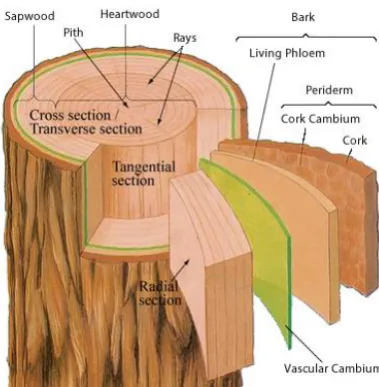
Figure 1-1: Schematic of tree stem (DoITPoMS, 2008) showing the main components of a tree stem. The wood tissue (xylem) consists of heartwood and sapwood, surrounded by the cambium layer where cell division takes place. ... 3
Figure 1-2: Example of annual tree-rings in (a) Scots pine – softwood, (b) Birch – Diffuse
porous hardwood, (c) Oak – Ring porous hardwood. Each ring represents one year of growth 4
Figure 1-3: Schematic representation of the principle behind cross-dating (Kaennel and Schweingruber, 1996), illustrating the use of tree-rings from sub-fossil samples, historic buildings and living trees. ... 5
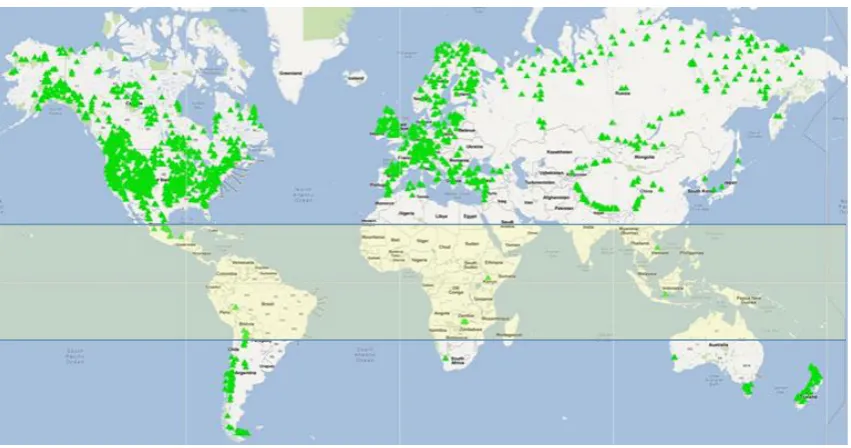
Figure 1-4: Visualisation showing the distribution of archived tree-ring chronologies around the world. Few chronologies have been produced in the tropics (highlighted in map) compared to in temperate regions. This map was created in Google Maps using data provided by ITRDB (2012) and map data by Google. ... 6
Figure 1-5: (a) Example of a false ring occurring in a conifer species (Brown, 2013). (b) Example of a wedging ring in a conifer species (Schweingruber, 2006). ... 8
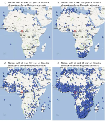
Figure 1-6: Visualisations showing the locations of climate stations in Africa. General location of the field site as described in Chapter 3 and Chapter 4 is represented by the red squares. Images were created using Google Maps. Map data was provided by Google, station data from KNMI Climate Explorer (http://climexp.knmi.nl/)... 9
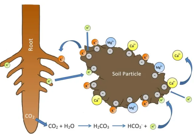
Figure 1-7: Image illustrating cation exchange on the surface of soil particles. Cations adsorb to the negatively charged surfaces of the soil particle by electrostatic attraction. Bound cations may be displaced into the soil solution by other cations with higher binding affinities, making them available for uptake by the roots. Image adapted from W. H. Freeman & Co. (No Date) and Taiz and Zeiger (2010). ... 24
Figure 1-8: Illustration representing the symplastic and apoplastic pathway for nutrient movement within the root. Ions are taken up by the epidermal cells, and transferred via the symplast or apoplast through the cortical and endodermal cells into the stele, where they are enter the xylem. In most cases (where present), the Casparian strip interrupts the apoplastic transport. Image adapted from Kimball (2013) ... 26
Figure 1-9: Schematic illustrating the role of membrane proteins in the transport of cations by primary and secondary active transport, and passive transport (White, 2012). ... 27
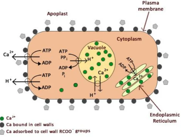
Figure 1-10: Diagram illustrating distribution of calcium in a cell and the transport processes
for sustaining low concentrations of cytosolic Ca2+. Figure based on Marschner (1995) and
Hindshaw et al. (2013). ... 35
x
Figure 2-2: Example of a sectioned rectangular lath for laser ablation analysis. Each section has been cut at an angle to allow rings to be overlapped on adjacent sections. ... 51
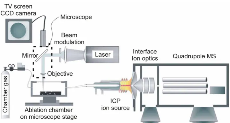
Figure 2-3: Illustration representing the typical configuration of a Laser Ablation-ICP-MS system. Image from Guillong (2007) ... 52
Figure 2-4: Plot of the raw data obtained from the continuous measurement of 44Ca by
LA-ICP-MS over a 10mm line along the radii of a Scots Pine lath. Two replicate lines were measured (red and blue) in the direction of growth (pith towards bark), with the mean of these represented by the black line. ... 54
Figure 2-5: Mean 44Ca plot from Figure 2-4 overlaid onto scanned image of the Scots pine
wood lath. The two lines measured are represented by the two dark burned lines in the wood. The highlighted peak does not correspond with a ring boundary. ... 55
Figure 2-6: The above plots show the mean and median raw 44Ca data obtained from the
analysis of 10 replicate lines for 3 separate sets of rings (A-C). Each plot has been superimposed onto a scanned image of the corresponding area from which the measurements were obtained. ... 56
Figure 2-7: Section of Scots pine lath showing the areas measured for the EW and LW tests (highlighted by the red box). ... 57
Figure 2-8: Plot showing the difference in counts between the earlywood and latewood regions as measured on a Scots pine sample. ... 58
Figure 2-9: Plots showing the 5 ablated lines plus the median of these for each of the four pelleted standards... 61
Figure 2-10: Graph shows the calcium output from the median of three ablated lines of Scots pine and the mean of 3 ablated lines of the NIST pine needles standard. Both y-axis scales are plotted with equal intervals for comparison. ... 63
Figure 2-11: Example of a sub-sectioned portion of a Scots pine lath showing the three replicated laser ablated tracks across the length of the section. ... 64
Figure 2-12: Plot of raw data for 44Ca isotope as measured by LA-ICP-MS for one section of
tree lath 05147. The Ca intensity is measures in counts per second, and the three lines plotted represent the 3 replicated tracked ablated across the lath section. The graph has been truncated for display purposes. ... 65
Figure 2-13: A scanned image of a section of analysed tree lath (tree 01547) with the associated raw 44Ca counts plotted and overlaid. The enlarged section highlights (blue circles) two of the resin ducts present on the laser track which corresponds to the calcium spike. ... 66
Figure 2-14: Figure showing the mean plot (a) and the median plot (b) of the 3 replicated 44Ca
xi
Figure 2-15: A Typical example of the drift observed over time (distance). (a) Plot showing the
median 44Ca (blue) data and the median 13C (red) data obtained from tree 05134 R2 D. (b) Plot
showing the ratio of the 44Ca/13C values for the same tree 01534 R2 D. ... 69
Figure 2-16: The median 44Ca/13C values (±2 standard error of the mean (SEM))are shown for
the four NIST standard measurements carried out on each of the five sections of a single pine tree lath (tree 05129) ... 69
Figure 2-17: (a) Graph showing the raw median 44Ca/13C values for all sections of tree 05135
R1 which had been split into 6 sections for analysis. (b) The same plot with low frequency filters overlaid onto each section illustrating the detrending functions which were applied to the data. These plots clearly illustrate the decreasing trend in calcium counts and the problems associated with section linkage. ... 73
Figure 2-18: (a) The resultant plot after each section was individually detrended using the filters illustrated in Figure 2-17. (b) The final, fully adjusted, values for tree 05135 R1 are represented here. Data for each section has been detrended as in (a) and converted to z-scores. ... 74
Figure 2-19: (a) Overlapping regions for two lath sections (tree 05135) after data has been detrended and converted to z-scores. (b) The same graphs have been overlaid onto the scanned image along with RW values for two of these rings. ... 76
Figure 2-20: The data for the outer section (G) of tree 05135 R1. The increase in Ca values highlighted on the graph represents the outer edge of tree where laser fires into bark... 78
Figure 2-21: The above graph shows the final, fully adjusted, values for tree 05135 R1 after the splicing of data into one single Ca dataset. Data for each section has been detrended as in (a) and converted to z-scores. ... 79
Figure 2-22: Image illustrating the three threshold values which were used to identify ring
boundaries from the 44Ca/13C data. Some peaks may only be identified as a boundary at the
lower threshold limits. Plot is showing data from tree 05135 R1 ... 81
Figure 2-23: Illustration highlighting the typical seasonal signal in calcium found across a growth ring. The plot represents the median values of 3 replicate lines (ablated lines are visible under the plot) ... 82
Figure 2-24: Example of the adjusted median 44Ca/13C values plotted with the ring widths
(green) and Ca years based on the >1 threshold (red) for tree (05134 R1). The data is split into two graphs for easier viewing. ... 84
Figure 2-25: Illustration of the three threshold values tested for assigning ring status to peaks for 05134 R1. The graph is split into two sections for easier viewing. The red diamonds show the results of designating Ca years based on the >1 threshold. The red oval denotes an area where there is a potential for more than 1 Ca year to be assigned for the 1 true year. ... 85
xii
Figure 3-1: (a) Map showing the general location of Mbam Djerem National Park in central Cameroon. (b) The yellow square in the centre of this map represents the fieldwork location within the park. The blue flags represent the locations of the nearest climate stations; Tibati is north, and Yoko is East of the park. Both maps were downloaded from Google Maps. ... 103
Figure 3-2: Average monthly rainfall data (±2 SEM) from the Tibati and Yoko weather stations (KNMI Climate Explorer, http://climexp.knmi.nl). Data has been averaged for each month for each year between 1940-1994 (data between 1994-present not available). ... 104
Figure 3-3: Example of Terminalia macroptera growing in the savanna. Most trees were found
to grow in this asymmetrical manner. ... 105
Figure 3-4: (a) Satellite image from 2006 showing the location of the field site within Mbam Djerem National Park (yellow box). The light areas represent savannah regions, darker green areas are forest and the Djerem river is pink. Image downloaded from USGS Global Visualisation (http://glovis.usgs.gov). (b) Shows a representation of the sampling locations (red dots) for the 5 trees in relation to the forest-savanna transition. ... 105
Figure 3-5: Shows the output radiocarbon plot obtained using the OxCal online calibration software available from https://c14.arch.ox.ac.uk/oxcal using the intcal13atmospheric curve (Reimer et al., 2013) ... 106
Figure 3-6: Graph showing the effect on the 14C levels in the Northern and Southern
Hemispheres caused by the weapons testing during the 1950’s and 60’s. The peak of the bomb spike is slightly lower and later in the southern hemisphere. Image from Earth System Research Laboratory (NOAA, 2012). ... 108
Figure 3-7: Example of Terminalia macroptera. The wood contains ring-like structures,
however there are not of a consistent nature. ... 109
Figure 3-8: Example of sub-sectioned portion of a T. macroptera lath showing the three
replicated laser ablated tracks across the length of the section. Each track is 0.2mm apart.. 111
Figure 3-9: Example of overlap region between tree 2A-R1 sections B and C as highlighted within the black box. ... 113
Figure 3-10: Example of applying 4-point smoothing function through the data. ... 114
Figure 3-11: Image shows the positions of the calcium assigned year comparisons made between each radius for tree 2A. The area where the wood has been removed represents the areas for two of the radiocarbon dates (2A-B and 2A-C), with the location of 2A-A radiocarbon dae indicated by the white arrow. The H/S boundary position is shown by the dashed line. 116
Figure 3-12: Scanned image of tree late 2Y after laser ablation analysis. Black arrows represent show 10 year increments as calculated using the >1.25 SD calcium threshold
technique. Red arrows repesent the locations for the 14C sampling based on the >1.25
threshold. The inner sampling location (2Y-Inner) is not shown here. ... 119
xiii
difficult to follow. (b) Shows an example of wedging, where banding pinches out resulting in incomplete banding around the circumference of the tree. ... 120
Figure 3-14: The above graphs plot the raw median 44Ca/13C values obtained for each of the
trees measured. H/S boundary regions (where present) are highlighted within the black rectangles. ... 122
Figure 3-15: The raw median 44Ca/13C data is shown here overlaid onto the section B of tree
2A-R1. An abrupt change in the data intensity is shown here which may be caused by the H/S transition area (highlighted in red). ... 123
Figure 3-16: Scanned image of T. macroptera (tree 2A) with plot showing 44Ca/14C signal for
this section overlaid on the image. The ring-like structres can be seen clearly. ... 125
Figure 3-17: (a) Graph showing the raw median 44Ca/13C values for all four sections of tree 2A.
Each section is plotted with the low frequency part of the Gaussian filter which was used to detrend each section. For section C, the data was detrended by 2 separate functions due to the large change in variance at ~40mm from the bark. (b) Graph showing the result of detrending each section using the detrending functions shown in (a). ... 128
Figure 3-18: (a) Graph showing the result of converting each lath section to z-scores. The overlapped regions are still present, but have been removed in (b). After data is spliced together (Section 3.3.3) the data is treated as one single dataset. ... 129
Figure 3-19: Section B of tree 2Y (a) shows the calcium spike in the data caused by the presence of the resinous substance which is highlighted in (b). ... 130
Figure 3-20: Both plots have been truncated for display purposes. (a) The raw median
44Ca/13C values for the 3 sections of tree 2Y are plotted with the low frequency part of the
Gaussian filter (detrending function). The effect that the single large calcium spike in section B has can be seen in (b) which shows the detrended data after conversion to z-scores. ... 131
Figure 3-21: These graphs show the result of removing the spike in data. (a) The raw median
44Ca/13C values for the 3 sections of tree 2Y are plotted with the low frequency part of the
Gaussian filter (detrending function). (b) results of detrending the data and conversion to z-scores after spike removal. The 3 sections are now in alignment and can be spliced together. ... 131
Figure 3-22: Plots showing Final calcium data obtained for each of the T. macroptera samples.
Two radii from sample 2A were analysed. ... 133
Figure 3-23: The above 3 plots show positions of calcium year assignment for tree 2A-R1, using the threshold >1. The graph is split into 3 sections and truncated for display purposes. The red diamonds represent the start of an annual growth season as determined by the assignment criteria, and the red line represents the threshold position. The arrows show the positions of the 14 tie points used for within tree error assessment. ... 135
xiv
criteria, and the red line represents the threshold position. The arrows show the positions of the 14 tie points used for within tree error assessment. ... 136
Figure 3-25: The plots (a-e) were produced using the online CALIBomb software which is available from http://calib.qub.ac.uk/CALIBomb/frameset.html. The calibration was carried out using the intcal13 calibration and Levin datasets, using a smoothing factor of 1.0 year. . 144
Figure 3-26: Graphical explanation of table layout ... 147
Figure 3-27: Graphical explanation of table layout ... 150
Figure 3-28: The plots (a-e) were produced using the online CALIBomb software which is available from http://calib.qub.ac.uk/CALIBomb/frameset.html. The calibration was carried out using the intcal13 calibration and Levin datasets, using a smoothing factor of 1.0 year. . 154
Figure 3-29: Graphical explanation of table layout ... 157
Figure 4-1: Satellite images showing locations of field sampling areas. (a) Positions of the two nearest climate stations to the field area are indicated by white arrows. Image acquired from Google Earth, Image data: Google, Landsat. (b) Shows approximate locations of individual sampling areas. Image acquired from Google Earth, Image data: Google, Cnes/Spot Image. 166
Figure 4-2: Photos representative of the savanna in the field site. (a) Shows trunk of T.
macroptera tree surrounded by tall grasses. (b) General view with T. macroptera trees in the background ... 167
Figure 4-3: Photos show the forest-savanna transitional boundary. (a) Shows the view from the savanna looking towards the forest. (b) shows the view from just inside the forest looking out towards the savanna... 168
Figure 4-4: Average monthly rainfall data (±2 standard error of the mean (SEM)) from the two closest weather stations to the field site and the gridded CRU TS3.1 ((Mitchell and Jones, 2005,
Harris et al., 2014). Precipitation data is shown from the period of 1940-1994 for the two
weather stations, and 1901-2009 for CRU dataset. Average monthly temperature data (±2 SEM includes the years 1901-2009 from CRU dataset... 169
Figure 4-5: Schematic representation of an (a) on-line TC/EA system for 18O measurements
(b) on-line EA system for 13C measurements. Images modified from (Scinco.com) ... 171
Figure 4-6: Schematic representation of an Isotope Ratio Mass Spectrometer ... 171
Figure 4-7: Oxygen isotope series for tree 2A, plotted by distance sampled along the tree’s radius. ... 177
Figure 4-8: Carbon isotope series for tree 2A, plotted by distance sampled along the tree’s radius. Data is uncorrected for Suess effect. ... 177
xv
Figure 4-10: Carbon isotope series for tree 2A. Data is plotted on calendar scale using growth
rates calculated from the 14C results. 13C has been corrected for Suess effect based on
(McCarroll and Loader, 2004) ... 180
Figure 4-11: The five plot show the original 18O data for tree 2A, followed by ‘seasonal
quaterly’ 18O series generated by the linear interpolation of the orginal series. The
correlations between each ‘season’ are shown as a representation of how this data relates to each other. ... 181
Figure 4-12: The five plot show the original 13C data for tree 2A, followed by the ‘seasonal
quaterly’ 13C series generated by the linear interpolation of the orginal series. The
correlations between each ‘season’ are shown as a representation of how this data relates to each other. ... 182
Figure 4-13: The four plots represent the seasonal precipitation (data from CRU TS 3.1
(Mitchell and Jones, 2005, Harris et al., 2014)) for 4 periods of the year. The correlations
between each season show the relationship between the data for each season. ... 184
Figure 4-14: The four plots represent the seasonal temperature (data from CRU TS 3.1
(Mitchell and Jones, 2005, Harris et al., 2014)) for 4 periods of the year. The correlations
between each season show the relationship between the data for each season. ... 185
Figure 4-15: The plot shows a comparison between the 18O season 2 and the temperature
season 2 series, with the first differenced versions of the same series (inverted for visual
comparison). A significant negative correlation was found only between the 1st diff. series
(r=-0.342). ... 187
Figure 4-16: The plot shows a comparison between the 18O season 3 and the precipitation
season 3 series, with the first differenced versions of the same series. A significant correlation was found only between the 1st diff. series (r=0.370) ... 187
Figure 4-17: The plot shows a comparison between the 18O season 4 and the precipitation
season 3 series, with the first differenced versions of the same series. A significant correlation was found only between the 1st diff. series (r=0.405) ... 188
Figure 4-18: The plot shows a comparison between the 13C season 2 and the precipitation
season 4, with the first differenced versions of the same series (series inverted for visual
comparison). A significant negative correlation was found only between the 1st diff. series
(r=-0.417). ... 189
Figure 4-19: The plot shows a comparison between the 13C season 3 and the precipitation
xvi
List of Tables
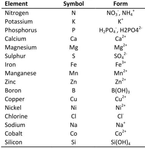
Table 1-1: List of essential mineral elements required for growth in higher plants (Fritter and Hay, 2002) ... 22
Table 2-1: Operating parameters for the LA-ICP-MS system used during initial tests. ... 54
Table 2-2: Composition of calcium standards. ... 60
Table 2-3: Final operating conditions which were manually set for LA-ICP-MS. Other parameters which are not listed here were determined by the automatic tuning procedures provided in the software. ... 60
Table 2-4: Table shows the coeffient of variation for each standard as calculated from the mean values from the 5 replicated lines. ... 62
Table 2-5: Comparison of the total distance measured from LA-ICP-MS analysis with the distance measured by CooRecorder along the same ablated tracks. The average difference between measurements is 0.19mm with the CooRecorder measurements always being slightly longer. ... 78
Table 2-6: Actual and estimated rings counts using the > 1 standard deviation threshold... 86
Table 2-7: Actual and estimated rings counts using the > 1.5 standard deviation threshold ... 86
Table 2-8: Actual and estimated rings counts using the > 2 standard deviation threshold... 86
Table 3-1: Results from the analysis of a single radiocarbon date obtained from the pith region
of a T. macroptera tree. Analysis was carried out by the Scottish Universities Environmental
Research Centre (SUERC), East Kilbride, Scotland. ... 106
Table 3-2: Operating parameters used for analysis of Terminalia macroptera. The spot size for
elemental measurements was reduced to 40µm/s however the preablation spot size was left at 100µm. ... 110
Table 3-3: The following tables show the results of the calcium assigned year comparisons when using (a) a threshold of > 1 st. dev. above the mean to mark annual increments and (b) a threshold of > 1 st. dev. above the mean to mark annual increments after a smoothing function has been applied to the data. ... 138
Table 3-4: The following tables show the results of the calcium assigned year comparisons when using (a) a threshold of > 1.25 st. dev. above the mean to mark annual increments and (b) a threshold of > 1.25 st. dev. above the mean o mark annual increments after a smoothing function has been applied to the data. ... 139
xvii
Table 3-6: The following tables show the results of the calcium assigned year comparisons when using (a) a threshold of > 2 st. dev. above the mean to mark annual increments and (b) a threshold of > 2 st. dev. above the mean o mark annual increments after a smoothing function has been applied to the data. ... 141
Table 3-7: Results from the radiocarbon dates from tree 2A. ... 143
Table 3-8: Calibrated radiocarbon dates for each of the samples from tree 2A. Radiocarbon
age was calculated using the online CALIBomb calibration software (Reimer et al., 2013)
available from http://calib.qub.ac.uk/CALIBomb/. The age ranges with the highest probability is highlighted in yellow. ... 143
Table 3-9: Shows a summary of the possible 14C dates obtained for the samples from tree 2A.
The calcium date range for each peak threshold was compared to the 14C ranges, and the
difference in years between the two ranges were calculated (Figure 3-26). The calcium ranges
which agree, or fall within the 14C date range are highlighted in yellow. ... 147
Table 3-10: The following table shows a summary of the possible 14C dates obtained for the
samples from tree 2A when using the troughs in the calcium data to represent an annual
increment. The calcium date range for each threshold was compared to the 14C ranges, and
the differences in years between the two ranges were calculated. The calcium ranges which agree, or fall within the 14C date range are highlighted in yellow. ... 150
Table 3-11: Results from the radiocarbon dates from tree 2Y. ... 153
Table 3-12: Calibrated radiocarbon dates for each of samples from tree 2Y. Radiocarbon age
was calculated using the online CALIBomb calibration software (Reimer et al., 2013) available
from http://calib.qub.ac.uk/CALIBomb/. The age ranges with the highest probability is highlighted in yellow. ... 153
Table 3-13: Shows a summary of the possible 14C dates obtained for four of the samples from
tree 2Y. The calcium date each threshold was compared to the 14C ranges, and the difference
in years between the two ranges were calculated (Figure 3-26). The calcium ages which agree, or falls within the 14C date range are highlighted in yellow. ... 157
Table 3-14: Information collected about physical properties of the two radiocarbon dated trees. Height was estimated using a Laser Vertex Hypsometer (Haglöf, Sweden). ... 158
Table 4-1: Precision is based on the average standard deviations for each standard analysed throughout all runs. ... 176
Table 4-2: Summary of 14C dates which were obtained for tree 2A (NERC allocation number
1562.0411). The 14C age ranges which have the highested probability are highlighted in yellow.
... 178
Table 4-3: Growth rates used to date the isotopic series. These were calculated based on 14C
dates for the tree ... 179
Table 4-4: Significant correlations found between the 18O data with relevant climate records.
xviii
Table 4-5: Significant correlations found between the 13C data with relevant climate records.
1
1.1.
Project Rationale
Dendrochronology is the study of the chronological sequence of annual growth rings in trees
(Stokes and Smiley, 1996). Traditional dendrochronological methods do not work well in most
tropical ecosystems making it difficult to study past changes in tropical climate, forest
productivity and stand dynamics. The principal barriers to using these traditional methods are
the lack of an obvious seasonality in many parts of the tropics and the absence of distinct
growth rings. Tree growth in many tropical locations is continuous throughout the year
(Worbes, 1999, 2002) resulting in trees with either indistinct incremental bands which are
generally non-annual in nature, or no ring-like structures at all. This situation means that the
dating of trees using traditional dendrochronological methods is almost impossible in most
tropical environments resulting in an inability to quantify tree-growth rates. In rare situations
distinct annual rings have been found in some species (Indonesia - D'Arrigo et al., 1994, Africa -
Trouet et al., 2001, 2006b, Schongart et al., 2006, Therrell et al., 2006). Such studies however
are relatively uncommon and tropical dendrochronology remains an elusive “Holy Grail” in
forest research and paleoclimatology.
As traditional dendrochronological methods do not work well in the tropics, alternative
methods of assessment have been used to determine growth rates in tropical trees. Such
methods include cambial wounding (Mariaux, 1967, Sass et al., 1995, Ohashi et al., 2009) and
dendrometer measurements, (Worbes, 1999, da Silva et al., 2002, Ohashi et al., 2009) both of
which can generally provide continuous growth rate data for the period of measurement.
Stable isotope analysis can also be used to develop records of seasonality, leading to the
possibility of dating tropical trees. In successful studies, correlations with seasonal rainfall
have been established; however the development of tropical chronologies (Evans and Schrag,
2004, Poussart and Schrag, 2005, Anchukaitis et al., 2008b) and climate reconstructions using
stable isotopes are still rare and the majority of successful studies in this field have used a
combination of stable isotope analysis combined with additional methods for assessing growth
rates.
Preliminary research over the last 10 years suggests that elemental analysis may address the
2
issues. Trees undergo many physiological processes during growth which require the uptake,
use and storage of many mineral elements. Since growth is affected by seasonality (no matter
how slight, whether temperature or precipitation controlled, this seasonality can be
represented in the element stores it uses for growth. Patterns of seasonality for some
minerals have shown potential for using these archives to develop a novel dating method for
tropical trees (Poussart et al., 2006) but little application of the approach has been made.
This thesis explores a novel dendrochemistry method to address the dating of tropical trees
using calcium as an indicator of seasonality. Calcium plays an important role in wood
formation, providing structure and rigidity to cell walls as well as being required for cell
division (Eklund and Eliasson, 1990, Martin et al., 2001, Lautner and Fromm, 2010). The link
between calcium and seasonality of tree growth has been investigated in temperate trees
(Follet-Gueye et al., 1998, Lautner and Fromm, 2010) as well as some exploratory work in the
tropics (Poussart et al., 2006). The severe limitation on dating using traditional based
dendrochronological methods in the tropics has led to a need for new approaches to open up
these tropical regions. Calcium is utilised in all trees and may provide a means to study growth
in trees where traditional methods do not work. Previous studies have investigated the
important role calcium plays in tree growth and development, methods for measuring calcium,
and have shown seasonal links. These studies have therefore demonstrated the potential for
calcium to be used as a seasonal indicator in tropical trees, which will be thoroughly explored
in this thesis.
Herein, calcium fluctuations were measured using Laser Ablation-Inductively Coupled
Plasma-Mass Spectrometry (LA-ICP-MS); a method that requires minimal preparation time as
wholewood cores can be used, and is also a relatively cheap and fast process. The sample size
is so small that the process is almost non-destructive and allows replicate measurements to be
easily obtained. In order to establish whether this method could be viable for application to
tropical trees, the concept was first evaluated using temperate trees with clear annual growth
rings as a positive control, as the rings could provide a robust secondary method of dating
using traditional dendrochronological methods. Pinus sylvestris (Scots pine) collected in the
Scottish highlands was chosen as it is a temperate species where growth increments follow a
clear annual pattern, therefore any seasonal patterns in the calcium measurements should be
3
indicated seasonality, the method was further refined for the detection of seasonal patterns
from calcium in ringless tropical species.
1.2.
Dendrochronology
As a tree grows it increases in circumference due to activity in the vascular cambium
(secondary growth) producing the woody part of the tree called the xylem (Figure 1-1).
Environmental factors such as seasonal variation, nutrient availability and related changes in
temperature and moisture availability influence the speed of growth.
Figure 1-1: Schematic of tree stem (DoITPoMS, 2008) showing the main components of a tree stem. The wood tissue (xylem) consists of heartwood and sapwood, surrounded by the cambium layer where cell division takes place.
Trees can be split into two broad basic types called gymnosperms (softwoods) and
angiosperms (hardwoods), with angiosperms further subdivided into monocots and dicots.
Monocots do not produce a vascular cambium and are therefore unsuited to
dendrochronological studies (Speer, 2010). Most other hardwoods and softwoods, when
growing in temperate regions, produce one tree-ring per year which consists of earlywood
(produced in spring/early summer) and latewood cells (late summer) which differ in structure.
The structural differences between cells can result in an abrupt transition in the xylem and can
be seen as a tree or growth ring in many trees; however this transition may take on different
[image:23.595.205.395.278.472.2]4
Figure 1-2: Example of annual tree-rings in (a) Scots pine – softwood, (b) Birch – Diffuse porous hardwood, (c) Oak – Ring porous hardwood. Each ring represents one year of growth
Tree growth can be affected by variations in climate which are recorded by patterns of narrow
and wide rings depending on the environmental conditions of the local area at that particular
time (Baillie, 1995, Stokes and Smiley, 1996). Surrounding trees will respond similarly to these
environmental factors thus providing the opportunity to link growth patterns between trees.
In regions where growth rings are laid down annually (e.g. temperate zones), the careful
measuring of ring widths and the cross-dating of ring width series of the same species can
determine the age of a tree. This process forms the basis of dendrochronology. Cross-dating
is the art of comparing separate ring width series by matching up patterns and sequences of
rings (Figure 1-3) allowing the synchronisation of individual tree-ring series into longer,
accurately calendar-dated chronologies (Douglass, 1941, Baillie, 1995). Dendrochronological
methods are not restricted only to living trees but can be applied to preserved sub-fossil wood,
dead wood and also historical wood such as from beams found in old buildings. In many cases
these pieces can be of key importance as living samples can be synchronised with dead
material of the same species allowing chronologies to be extended back much further in time
to produce very long accurately dated chronologies (Stokes and Smiley, 1996, Eronen et al.,
2002, Grudd et al., 2002, Helama et al., 2008).
Dendrochronology has varied uses such as providing a tool for historical dating (Baillie, 1995,
5
reconstructions (Cook et al., 2004, Buntgen et al., 2005, Luckman and Wilson, 2005, D'Arrigo et
al., 2006a, Esper et al., 2007, Wilson et al., 2007). Establishing accurately dated chronologies is
the basis for all disciplines of dendrochronology. The reconstruction of climate is possible by
using available climate data from meteorological stations near to the study sites, evaluating
the relationships between the instrumental data and ring widths and applying these
relationships to reconstruct climate data for these areas over the length of the chronologies.
These methods have been used with great success for assessing the variability in historic
climate trends and are very important for late Holocene Palaeoclimate reconstructions,
providing spatial patterns of inter-annual climate variability on regional and global scales
(Jansen et al., 2007, Jones et al., 2009).
[image:25.595.97.505.327.619.2]6
1.3.
Dendrochronology in the Tropics
Thousands of tree-ring chronologies exist in temperate regions (ITRDB, 2012)1 however this is
not the case in the tropics (Figure 1-4). The existence of clearly defined tree-rings in tropical
trees has been long debated, despite evidence to the contrary, leading to a general belief that
the tropics typically lack sufficient seasonality to produce annual growth rings (Lieberman et
al., 1985, Worbes, 1995, Whitmore, 1998, 2002, McCarroll and Loader, 2004). Worbes (2002)
reviewed the progress of tropical dendrochronology and highlighted that as far back as 1900,
Ursprung (1900) had observed the link between the seasonality of tropical tree growth and its
relationship to cambial activity. The first tropical tree-ring chronology was produced by
Berlage in 1931 from Indonesian Teak (Tectona grandis L.f.) for a period of over 400 years
(Berlage, 1931) and demonstrated relationships between dry season precipitation and wet
monsoon seasons (D'Arrigo et al., 1994). This chronology was extended over 60 years later by
D’Arrigo et al. (1994) increasing the chronology length to almost 500 years.
Figure 1-4: Visualisation showing the distribution of archived tree-ring chronologies around the world. Few chronologies have been produced in the tropics (highlighted in map) compared to in temperate regions. This map was created in Google Maps using data provided by ITRDB (2012) and map data by Google.
In an attempt to encourage the expansion of research and chronology development in the
tropics, Stahle (1999) produced a strategy guide for the successful development of tropical
1
[image:26.595.86.512.381.605.2]7
tree-ring chronologies. Where possible, it was suggested to use a species which has been
previously identified as suitable for dendrochronological studies or a member of its botanical
family, but where this was not possible, to refer to descriptions of wood anatomy to identify a
suitable species. Due to the lack of dendrochronological studies in the tropics, knowledge
regarding the suitability of different species is limited. Tarhule and Hughes (2002) recognised
this lack of information for dendrochronological research and carried out a suitability study in
West Africa using 600 trees, from 22 botanical families, 43 genera and over 70 species.
Samples were classified into three categories of ‘potentially useful’, ‘problematic’ and ‘poor’
which resulted in 7 species being categorised as potentially useful, 8 as problematic, and the
rest as poor. While this study showed the potential for applying traditional
dendrochronological methods to several tropical species, it more importantly highlighted the
difficulties associated with finding suitable species for such studies. Where information
regarding species suitability is available, consideration for the environmental conditions and
locality should also be taken into account as the same species found in a one area of the
tropics, may respond differently when growing in a different tropical climate.
In temperate trees, an annual ring is produced by the seasonal cycle’s influence on cambium
activity, where conditions suitable for growth are contrasted against dormancy brought on by
stressful conditions such as cold winters. Although many tropical regions do exhibit some
seasonality, this is more reflected by changes in precipitation and relative humidity rather than
temperature, which may remain relatively constant through the year. Cambial dormancy in
the tropics can be induced by prolonged dry periods or by more extreme conditions such as
periods of continued flooding (Worbes, 1995), but in many cases, the changes in seasonality
may not be large enough to result in distinct annual rings being formed (Poussart and Schrag,
2005). The climate in the inner tropics is often described as everwet, which is based on
precipitation records showing rainfall all year round (Worbes, 2002). Such conditions may not
provide the stressful environment required by the trees to result in annual or seasonal
banding. However, seasonality has been demonstrated in some regions when the recorded
monthly precipitation was so low that cambial dormancy was induced. Fichtler et al. (2003)
studied eight tree species from La Selva, Costa Rica, and observed that all formed visible
annual growth rings. La Selva is classified as an everwet region which experiences
precipitation all year round, but there are periods (averaging 12 days) without substantial
rainfall (<5mm). They reported that the formation of these annual rings could not be due to
8
drought stress resulting from these short lived drier periods which caused soil moisture
content to drop significantly triggering growth dormancy in the trees. These results indicate
that traditional dendrochronological studies can be applied even in areas of the tropics which
appear to lack any obvious seasonality.
Although it is clear that distinct annual rings are present in some tropical species, tropical
dendrochronology presents further challenges. The occurrence of growth ring irregularities
(Figure 1-5) such as false rings, missing rings or wedging rings (where a complete ring has not
been formed around the tree) is common (Tarhule and Hughes, 2002). These can be caused by
stress events such as drought or physical damage and require care be taken when attempting
to cross-date. Such problems aren’t unique to tropical trees. However, extreme climatic
conditions in tropical regions may make these ring anomalies more frequent, and where ring
width variability is low, cross-dating may be difficult or in some cases impossible (Fritts, 1976).
To complicate matters further, some tropical tree-ring studies have also reported the
occurrence of more than one ring per year (Gourlay, 1995) caused by more than one stress
event such as a second dry season, and also irregular ring formations (Sass et al., 1995).
(a) (b)
Figure 1-5: (a) Example of a false ring occurring in a conifer species (Brown, 2013). (b) Example of a wedging ring in a conifer species (Schweingruber, 2006).
Long tree-ring chronologies are needed to study past climatic variability of regions in the
tropics. Over Africa, the network of climate stations is sparse and in most cases the data is
relatively short (around 100 years) and spatially incomplete (Figure 1-6); therefore an
alternative solution is needed for understanding past climates and to expand on the available
instrumental data. Tree-ring chronologies could provide valuable inter-annual information for
9
trees producing annual rings and tropical dendrochronology could offer this solution.
Although the strong potential for applying traditional dendrochronological methods in the
tropics has been demonstrated with the successful construction of tree-ring chronologies, in
reality the application of these methods are still rare and success has been limited.
(a) Stations with at least 100 years of historical observations of monthly temperature data
(b) Stations with at least 100 years of historical observations of monthly precipitation data
(c) Stations with at least 50 years of historical observations of monthly temperature data
(d) Stations with at least 50 years of historical observations of monthly precipitation data
[image:29.595.88.519.171.671.2]10
Some tree ring chronologies have been developed in the tropics but far fewer than in
temperate regions and the time span covered is also shorter. Stahle et al. (1999) analysed
Pterocarpus angolensis in Zimbabwe and found that the ring anatomy showed distinct
boundaries and the ring width was highly correlated with wet season precipitation. This work
was extended by Therrell et al. (2006), where they developed a 200 year long regional
chronology and the first tree ring based precipitation reconstruction in tropical Africa. Fichtler
et al. (2004) used Pterocarpus angolensis and Burkea africana to develop short, site specific
chronologies (between 60 and 100 years) for two separate dry forests (900Km apart) in
Namibia. Correlations between ring width and precipitation were observed for both species at
both sites, as well as strong correlations with temperature and relative humidity for
Pterocarpus angolensis at one of the sites.
In South America, Schongart et al. (2004) developed the first ENSO2-sensitive dendroclimatic
proxy of the Amazon basin for Piranhea trifoliata. This 200 year chronology allows the dating
of El Nino events which happened prior to instrumental records, and indicated that the
severity of these events has significantly increased over time. In a different study, Schongart
et al. (2005) developed chronologies in Central Amazonia of Macrolobium acaiifolium from
two different floodplain types. From the nutrient-poor floodplain, an almost 400 year
chronology was produced, and from nutrient-rich floodplains, a 146 year chronology was
developed. Trees growing in the nutrient-poor floodplain were found to have significantly
more rings than similar sized (DBH3) trees growing in the nutrient-rich floodplain with the
nutrient poor trees also living longer. Both chronologies were significantly correlated with the
non-flooing period and increased wood growth was found to occur during El Nino events,
however the climate-growth relationship between this species and ENSO were less distinct
than found in the previously mentioned study. Success in the North American tropics has seen
the production of a 400 year chronology for Mexican mountain pine, Pinus hartwegii, in
Nevado de Colima, Mexico (Biondi, 2001). This study included trees of up to 500 years old,
despite past logging events in the area. The strongest correlated climate signal was for
summer monsoon precipitation which occurs in June, which is also when the transition from
the dry to the wet season occurs.
2
El Niño–Southern Oscillation
3
11
The above successes in tropical dendroclimatology illustrate the potential for such studies.
However this requires either prior knowledge of suitable species, a willingness to carry out
pilot studies or a wider sampling approach which in either case does not guarantee success.
With the complications that can arise from using traditional dendrochronological methods in
the tropics, other methods have been explored to assist in establishing growth rates and
seasonality on tropical trees, or as alternatives to traditional dendrochronological methods
where these may not be possible due to complications such as indistinct rings.
1.3.1. Measuring Growth Rates in Tropical Trees
Measuring the growth rates of tropical trees could provide a method of establishing dating
control for tropical species which lack visible annual rings. Annual incremental growth can be
measured by cambial wounding (Mariaux, 1967) which, as the name suggests, involves
physically wounding the tree stem at specific dates creating scarring on the xylem as the tree
continues growing around the wound. Sass et al. (1995) used this method, with mixed success,
to study the growth of two Malaysian tree species, Dryobalanops sumatrensis and Shorea
leprosula , over a period of four years by wounding the tree stems every two months. In both
species, relatively large areas of callus tissue formed around the wounded areas, which was
complicated further with them having particularly slow growth rates as well as highly variable
cambial activity across the tree stems. Despite these issues, it was shown for D. sumatrensis
that wood formation was continuous throughout the year. It is clear however that this
method presents many challenges that require consideration prior to use in the tropics but the
major concern for using this method to establish growth rates is that ultimately the tree needs
to be felled in order to visualise all the scars and to assess the rate of growth. This may make it
unsuitable in areas where felling trees would not be permitted and also effectively ends that
particular chronology.
Cambial wounding results in scarring around the wounded area as the tree recovers, which
would not be desirable if further analysis were to be performed on the tree, especially as the
tree needs to be cut to view the growth around the scars. Dendrometer bands (Drew and
Downes, 2009) offer an alternative non-destructive method to measure growth rates in situ.
Measurements can be taken by attaching metal dendrometer bands around tree stems which
12
in place. Worbes (1999) used dendrometer measurements on different tropical species from
Venezuela to determine growth rates and seasonality, and showed that cambial activity stops
at the start of the dry season, and recommences during the wet season. This approach was
also implemented by da Silva et al. (2002) to assess the growth patterns of trees in relation to
rainfall growing over two sites in Central Amazon. Dendrometer measurements spanning 12
months, from 272 trees, were used to assess their growth patterns and calculate mean annual
diameter increment for the Brazilian Amazon region. While they reported that this provided
an accurate way to monitor and assess individual tree growth, it was noted that the particular
bands used could only monitor a 20mm expansion in diameter growth before requiring to be
changed which then required a lengthy adjustment period. This expansion size may vary
depending on the construction of the bands, however all bands do require a period of
adjustment to minimise any source of errors once the band has been set in place.
Dendrometer bands allow non-destructive measurement of tree growth over the period of
time they are in place. Advances in these measurement techniques have allowed variations of
dendrometers to be developed including bands that use data loggers to remotely take
accurate measurements at specific times (Drew and Downes, 2009).
Cambial wounding and dendrometer bands both provide methods of monitoring the growth
rates of trees which could assist in the dating of trees in the tropics. However each have
limitations as discussed, with the biggest one being that these methods can only assess growth
rates and trends over the period of measurement which covers only a very small percentage of
a tree’s life. Cambial wounding also requires the tree to be felled to view the resultant
scarring, but does provide a very cheap way to monitor growth. Such methods would be
ideally used in species suitability studies when little information is available about the trees in
a certain area.
1.4.
Dendrochemistry
Dendrochemistry is the study and interpretation of the different elements in tree-rings. This
can include measurements of stable isotopes and other elements which can be taken up into a
tree and stored within the woody tissue. The basic premise is that these stores of chemicals
can be accessed from tree-rings and may be indicators of past chemical fluctuations in the
13
to building tree-ring chronologies and reconstructing past climates, as well as offering a wealth
of additional information regarding the environmental conditions affecting the tree’s growth.
Dendrochemistry should not be thought of as a replacement for traditional
dendrochronological methods as ring width measurements still provide the ‘best’ solution for
dating trees and climate reconstructions with the added advantage of being a relatively cheap
and fast solution, but as not all trees are amenable to ring width measurements (Section 1.3),
such as in the tropics, additional methods are required to extract potential information stored
within trees.
1.4.1. Stable Isotopes in Tree-Rings
The three main elements in wood are carbon, oxygen and hydrogen. Each of these contains
isotopes which are forms of the same element differing only by mass (due to having a different
number of neutrons). Carbon has two stable isotopes (12C and 13C) and one radioactive
isotope (14C), oxygen has three stable isotopes (16O, 17O and 18O), and hydrogen has two stable
isotopes (1H and 2H, also called H and D) and one radioactive isotope (3H). The stable isotopes
of an element have almost identical chemical properties. However the slight differences in
masses between them can cause chemical, biological and physical processes to discriminate
against one of them thereby altering the proportions in which they are present.
Carbon enters the tree as CO2 from the air and both oxygen and hydrogen enter via the tree’s
roots from soil water. The elements aren’t simply stored in these states, but undergo changes
from physiological processes resulting from the tree’s response to the climatic conditions at
that particular time. An understanding of these fractionation factors presents us with the
potential to use these natural stores to develop records of environmental change.
1.4.1.1. Stable Isotope Notation
Stable isotopes are reported as a ratio, relative to a standard. The ratio (R) of carbon, oxygen
and hydrogen isotopes are measured as the abundance of the rare isotope to that of the
common isotope and reported relative to the isotope ratio of a standard as follows (Farquhar
14
(
)
where is the element, is the atomic mass of its heaviest isotope. The value is multiplied
by 1000 and reported in parts per thousand (‰ or per mil).
1.4.1.2. Carbon Isotopes
Carbon isotopes are expressed as 13C which represents the observed 13C/12C ratio relative to a
standard. The standard for carbon isotope ratios was originally a fossil belemnite from the Pee
Dee formation of south Carolina (PDB) but has since been replaced by Vienna-PDB (VPDB) due
to the supply of the original PDB being exhausted (Coplen, 1995).
Trees take in carbon dioxide (CO2) from the air by diffusion through the stomata in the leaves.
During the intake, CO2 is fractionated in preference to the lighter carbon isotope (12CO2) by
~-4.4‰ making the internal air depleted in 13C relative to the external air. Photosynthesis causes
the internal CO2 to be further fractionated by ~-27‰ during carboxylation where the lighter
12
CO2 molecules are preferentially used to produce sugars (Loader et al., 2007). The
discrimination against the heavier carbon isotope (13C) during these processes can be
expressed as:
( )(
⁄
)
where a is the discrimination against the heavier isotope through the stomata, b is the
discrimination from carboxylation and ci and ca are the internal and external CO2
concentrations (Farquhar et al., 1982).
The dominant environmental conditions that affect carbon isotopic fractionation are those
that affect the rates of photosynthesis (light and leaf temperature) and stomatal conductance
15
1.4.1.3. Oxygen Isotopes
Oxygen isotopes are expressed as 18O which represents the observed 18O/16O ratio relative to
a standard. The standard for oxygen isotope ratios when measuring carbonates is usually the
same as used for carbon, Vienna-PDB (VPDB), however for the measurement of waters, ice
and plant material, the standard is Vienna Standard Mean Ocean Water (Vienna-SMOW or
VSMOW), which replaced the original Standard Mean Ocean Water (SMOW).
Trees get their water from soil moisture. The isotopic signatures of precipitation will therefore
play a part in the water isotopes stored in the wood, however fractionation by evaporation
(loss of lighter isotope 16O) in the soil can occur before water has entered the tree. Roots take
in soil water and transport it up to the leaves through the xylem. No fractionation occurs
during the transport (Evans and Schrag, 2004); the critical site of fractionation is in the leaf
(McCarroll and Loader, 2004). The loss of the lighter oxygen isotope, at the first fractionation
step, is caused by transpiration (Barbour et al., 2001). This occurs when the stomata open
either to allow in CO2 for photosynthesis or in response to climatic variables such as wind
speed or atmospheric humidity and H2O diffuses out. The first fractionation step of oxygen
means that since the leaf has a higher 18O than the surrounding environment, it is not simply
a matter of the tree giving a “snapshot” of the isotopic ratio of soil water but rather a means
by which we can deduce the temporal conditions from the given ratio. This can be achieved
by:
( )
where * is the resulting water vapour pressure caused by the heavy H218O, k represents the
fractionation caused by transpiration, 18Ov is atmospheric isotope ratio of water vapour
relative to source water and ea & ei is the ambient intercellular vapour pressure (Barbour et al.,
2001, McCarroll and Loader, 2004). Atmospheric conditions, mainly temperature, affect *
however the main factors affecting the 18O are the variations in the isotopic content of the
source water (soil water) and the vapour pressure differences between the internal and
external leaf.
Sucrose is formed within the leaf resulting in an enrichment in 18O by 27‰ due to the
exchange of carbonyl oxygen in organic molecules with water (Sternberg et al., 1986). During