Investigations into the Effect of Spatial Correlation on Channel Estimation and Capacity of Multiple Input Multiple Output System

(1)

doi:10.4236/ijcns.2009.24029 Published Online July 2009 (http://www.SciRP.org/journal/ijcns/).

Investigations into the Effect of Spatial Correlation on

Channel Estimation and Capacity of Multiple Input

Multiple Output System

Xia LIU1, Marek E. BIALKOWSKI2, Feng WANG1

1_{Student Member IEEE, School of ITEE, The University of Queensland, Brisbane, Australia} 2_{Fellow IEEE, School of ITEE, The University of Queensland, Brisbane, Australia}

Email: {xialiu, meb, fwang}@itee.uq.edu.au

Received December 17, 2008; revised March 28, 2009; accepted May 25, 2009

ABSTRACT

The paper reports on investigations into the effect of spatial correlation on channel estimation and capacity of a multiple input multiple output (MIMO) wireless communication system. Least square (LS), scaled least square (SLS) and minimum mean square error (MMSE) methods are considered for estimating channel properties of a MIMO system using training sequences. The undertaken mathematical analysis reveals that the accuracy of the scaled least square (SLS) and minimum mean square error (MMSE) channel estimation methods are determined by the sum of eigenvalues of the channel correlation matrix. It is shown that for a fixed transmitted power to noise ratio (TPNR) assumed in the training mode, a higher spatial correlation has a positive effect on the performance of SLS and MMSE estimation methods. The effect of accuracy of the estimated Channel State Information (CSI) on MIMO system capacity is illustrated by computer simulations for an uplink case in which only the mobile station (MS) transmitter is surrounded by scattering objects.

Keywords: MIMO, Channel Estimation, Channel Capacity, Spatial Correlation, Channel Modelling

1. Introduction

In recent years, there has been a growing interest in mul-tiple input mulmul-tiple output (MIMO) techniques in rela-tion to wireless communicarela-tion systems as they can sig-nificantly increase data throughput (capacity) without the need for extra operational frequency bandwidth. In order to make use of the advantages of MIMO, precise channel state information (CSI) is required at the receiver. The reason is that without CSI decoding of the received sig-nal is impossible [1–5]. In turn, an inaccurate CSI leads to an increased bit error rate (BER) that translates into a degraded capacity of the system [6–8].

Obtaining accurate CSI can be accomplished using suitable channel estimation methods. The methods based on the use of training sequences, known as the training- based channel estimation methods, are the most popular. In [9,10], several training-based methods including least square (LS) method, scaled least square (SLS) method and minimum mean square error (MMSE) method have

been investigated. It has been shown that the accuracy of the investigated training-based estimation methods is influenced by the transmitted power to noise ratio (TPNR) in the training mode, and a number of antenna elements at the transmitter and receiver. In particular, it has been pointed out that when TPNR and a number of antenna elements are fixed, the SLS and MMSE methods offer better performance than the LS method. This is due to the fact that SLS and MMSE methods utilize the chan-nel correlation in the estimator cost function while the LS estimator does not take the channel properties into account.

(2)

between spatial correlation and channel estimation accu-racy has been shown. The works presented in [11,12] have reported on the relationship between spatial corre-lation and estimation accuracy of MMSE method. How-ever, only simulation results, giving trends without any further mathematical insight have been presented.

In this paper, we try to fill the existing void by pre-senting the mathematical analysis explaining the effects of channel properties on SLS and MMSE channel esti-mation methods. It is shown that for a fixed TPNR, the accuracy of SLS and MMSE methods is determined by the sum of eigenvalues of channel correlation matrix, which in turn characterizes the signal propagation condi-tions. In addition, we report on the effect of spatial cor-relation on both the channel estimation and capacity of MIMO system. In the work presented in [13–16], it has been shown that the existence of spatial correlation leads to the reduced MIMO channel capacity. However, these conclusions rely on the assumption of perfect CSI avail-able to the receiver. In practical situations, obtaining perfect CSI can not be achieved. Therefore, in this paper we take imperfect knowledge of CSI into account while evaluating MIMO capacity.

The rest of the paper is organized as follows. In Sec-tion 2, a MIMO system model is introduced. In SecSec-tion 3, LS, SLS and MMSE channel estimation methods are described and the channel estimation accuracy analysis is given. Section 4 shows derivations for the lower bound of MIMO channel capacity when the channel estimation errors are included. Section 5 describes computer simu-lation results. Section 6 concludes the paper.

2. System Description & Channel Model

We consider a flat block-fading narrow-band MIMO sys-tem with Mt antenna elements at the transmitter and Mr antenna elements at the receiver. The relationship between the received and transmitted signals is given by (1):

s

Y HS V (1)

where Ys is the Mr× N complex matrix representing the received signals; S is the Mt× N complex matrix repre-senting transmitted signals; H is the Mr × Mt complex channel matrix and V is the Mr× N complex zero-mean white noise matrix. N is the length of transmitted signal. The channel matrix H describes the channel properties which depend on a signal propagation environment. Here, the signal propagation is modeled as a sum of the line of sight (LOS) and non-line of sight (NLOS) components. As a result, the channel matrix is represented by two terms and given as [17,18],

1

1 NLOS 1 LOS

K

H H H

K K

 

  (2)

where HLOS denotes the LOS part as and HNLOS denotes NLOS part. K is the Rician factor defined as the ratio of power in LOS and the mean power in NLOS signal component [17]. The elements of HLOS matrix can be written as [18]

) 2

exp( _rt

rt

LOS j D

H

 



 (3)

where Drt is the distance between t-th transmit antenna and

r-th receive antenna. Assuming that the components of NLOS are jointly Gaussian, HNLOS can be written as [19,20],

2 / 1 2 / 1

T g R NLOS R H R

H  (4)

where Hg is a matrix with i.i.d Gaussian entries.

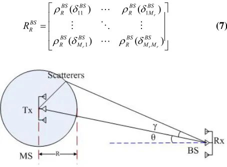
Here, the Jakes fading model [21,22] is used to de-scribe the spatial correlation matrices RR at the receiver and RT at the transmitter. An uplink case between a base station (BS) and a mobile station (MS) is assumed, as shown in Figure 1.

The BS antennas are assumed to be located at a large height above the ground where the influence of scatterers close to the receiver is negligible. In turn, MS is assumed to be surrounded by many scatterers distributed within a “circle of influence”. For this case, the signal correlation coefficients at the receiver BS and transmitter MS, ρRBS and ρTMS_{, can be obtained from [22] and are given as:}

0

( ) [2 / ]

MS T T

T mn J mn

     (5)

0 max

2 2

( ) [ cos( )]exp( sin( ))

BS R R R

R mn J mn j mn

 

     

 

  

(6)

where, δmnT_and _δmnR_{are the antenna spacing distances} between m-th and n-th antennas at transmitter and re-ceiver, respectively; λ is the wavelength of the carrier; γmax is the maximum angular spread (AS); θ is the AoA of LOS and J0 is the Bessel function of 0-th order. Using ρRBS₍_δmnT₎_and_ρTMS₍_δmnR₎_{, the correlation matrices}_R

R

r

M

BS and RTMS for BS and MS links can be generated as

11 1

1

( ) ( )

r

r r

BS BS BS BS

R R

BS R

BS BS BS BS

R M R M M

R

   

 

 

  

 

 



  



[image:2.595.311.538.539.706.2]

(7)

(3)

AND CAPACITY OF MULTIPLE INPUT MULTIPLE OUTPUT SYSTEM

t

M 

  

11 1

1

( ) ( )

t

t t

MS MS MS MS

T T

MS T

MS MS MS MS

T M T M M

R

   



 

   



  



(8)

3. Training-Based Channel Estimation

For a training based channel estimation method, the rela-tionship between the received signals and the training sequences is given by Equation (1) as

Y HP V (9)

Here the transmitted signal S in (1) is replaced by P, which represents the Mt × L complex training matrix (sequence). L is the length of the training sequence. The goal is to estimate the complex channel matrix H from the knowledge of Y and P.

The transmitted power in the training mode is assumed to be constrained by P2_F where P is a constant and ||.||F2 stands for the Frobenius norm. According to [9,10],

the estimation using LS, SLS or MMSE method requires orthogonality of the training matrix P. In the undertaken analysis, the training matrix P is assumed to satisfy this condition.

 

3.1.

LS Method

In the LS method, the estimated channel can be written as [23],

†

ˆ LS

H YP (10)

where {.}†_{stands for the pseudo-inverse operation.} The mean square error (MSE) of LS method is given as

2

ˆ {

LS LS _F}

MSE E H H (11)

in which E{.} denotes a statistical expectation. According to [9,10], the minimum value of MSE for the LS method is given as

2

min

LS M Mt r

MSE



 (12)

in which ρ stands for transmitted power to noise ratio (TPNR) in training mode. Equation (12) indicates that the optimal performance of the LS estimator is not in-fluenced by channel matrix H.

3.2.

SLS Method

The SLS method reduces the estimation error of the LS method. The improvement is given by the scaling factor γ which can be written as

{ }

H

LS H

tr R

MSE tr R

 

 (13)

The estimated channel matrix is given as [9], [10]

†

2 1

{ } ˆ

{( ) } { }

H

SLS H

n r H

tr R

H YP

M tr PP tr R

 



  (14)

Here, σn2_{is the noise power;}_R

H is the channel correla-tion matrix defined as RH=E{HHH} and tr{.} implies the trace operation. The SLS estimation MSE is given as [9,10]

2

2 2

ˆ

{ }

(1 ) { }

SLS LS _F

H LS

MSE E H H

tr R MSE



 

 

   (15)

The minimized MSE of MMSE method can be written as [9,10]

min

{ } { }

SLS LS H

LS H

MSE tr R MSE

MSE tr R



 (16)

By taking into account expression (12), the minimized MSE of the SLS method (16) can rewritten as

1 1

2

1 2

1 1

2

[( { }) ]

[( ) ]

SLS H

t r

t r n

i

i t r

MSE tr R

M M

tr

M M

1

 

 

 



 

 

  







 (17)

where n=min(Mr, Mt) and is λi the i-th eignvalue of the channel correlation RH.

If TPNR is fixed then the following equality can be derived

1 1

2

[( n ) ] n

SLS i i

i t r i

MSE

M M 

   





 



(18)

As observed from (18), MSE decreases when the sum of eignvalues of RH decreases. This shows that in order to minimize MSE, the sum of eigenvalues of RH has to be reduced.

3.3.

MMSE Method

In the MMSE method, the estimated channel matrix is given as (19) [9,10,23],

2 1

ˆ ₍ H ₎ H

MMSE H n r H

H _Y P R P_ M I  P R

(19)

(4)

2

ˆ

{ } { }

MMSE MMSE _F E

MSE E H H tr R (20)

in which RE is an estimation error correlation written as

1 2 1 1

ˆ ˆ

{( )( ) }

( )

H

E MMSE MMSE

H

H n r

R E H H H H

R M PP 

  

  (21)

The minimized MSE is given as (22) [2,3,11]

1 2 1 1

{( H H ) }

MMSE n r

MSE _tr _{ } M Q PP Q  (22)

In (22), Q is the unitary eigenvector matrix of RH and

Λ is the diagonal matrix with eigenvalues of RH. The minimized MSE for the MMSE method, given by Equa-tion (22), can be rewritten using the orthogonality prop-erties of the training sequence P and the unitary matrix Q, as shown by

1 1 1

1

1 1 1

2

1 1 1

2

1 1 1

{( ) }

( ) 0 0

0 ( )

{

0

0 0 (

( )

MMSE r

r

r n

i r

i

MSE tr M I

M

M tr

M

  

 

   

  

  

 

 _ 



 _



 









 

  



}

)     

(23)

Assuming that TPNR in expression (13) is fixed, the bound for MSE is given by

1 1 1

( )

n n

MMSE i r i

i i

MSE _



 _M  _



_ (24)

The expression (24) shows that, similarly as in the SLS method, a smaller sum of eigenvalues of the channel correlation RH leads to a smaller estimation error for the MMSE method. In other words, a smaller sum of eigen-values of the channel correlation leads to the more accu-rate channel estimation.

From the above mathematical analysis it becomes ap-parent that when the value of TPNR is fixed the accuracy of a training-based MIMO channel estimation is governed by the sum of eigenvalues of the channel correlation matrix RH. In turn, the properties of RH and its eigenvalues are determined by the channel properties which are influenced by a signal propagation environment and an array antenna elements and configuration.

It is worthwhile to note that the spatial correlation (for example due to the presence of LOS component) is re-sponsible for the channel rank reduction. In this case, the sum of eigenvalues of RH has a smaller value. Thus from the derived expressions, it is apparent that the spatial cor-relation (due to an increased LOS component) contributes in a positive manner to improving the training-based MIMO channel estimation accuracy.

4. MIMO Channel Capacity Taking into

Account Channel Estimation Errors

The achievement of high channel capacity in a MIMO system depends on two factors. One is a rank of channel matrix or effectiveness of freedom (EDOF). The other one is the availability of CSI at the receiver. In [26,27,29] it has been shown that higher accuracy of CSI leads to higher channel capacity. However, the undertaken inves-tigations have not considered the channel properties.

If CSI is perfectly known at the receiver (but unknown at the transmitter), the capacity of a MIMO system with Mr receive antennas and Mt transmit antennas can be expressed as [1,24,25],

2

(log {det[ _R SNR( H)]}) M

t

C E I HH

M 

  (25)

In Equation (25), ρSNR is a signal to noise ratio (SNR). The channel matrix H is assumed to be perfectly known at the receiver.

In practical cases, H has to be replaced by the esti-mated channel matrix, which carries an estimation error. By assuming that the channel estimation error is defined as e and the estimated channel matrix as Hˆ

ˆ

HH e (26)

The received signal can accordingly be written as,

ˆ

Y HS eS V  (27)

Correlation of e is given as

2

ˆ ˆ

{( )( ) }H

E e

R E H H H H   I (28)

in which σe2 _{is the error variance. In [26,27], the}

defini-tion of error variance is slightly different. Using Equa-tion (20), we have

2 e

r

MSE M

  (29)

The channel capacity of MIMO system with an imper-fectly known H at the receiver is defined as the maximum mutual information between Y and S and is given as

{ }

ˆ max { ( ; , )}

tr Q P

C I S Y



 H

ˆ

(30)

If the transmitter does not have any knowledge of the estimated channel, the mutual information in Equation (30) can be written as [26–29],

ˆ ˆ ˆ

( ; , ) ( ; | ) ( | ) ( | , )

I S Y H I S Y H h S H h S Y H (31)

(5)

[image:5.595.325.531.123.257.2]

ˆ ˆ

( | , ) ( | , )

h S Y H h S uY Y H (32)

in which u is the MMSE estimator given as

ˆ

{ |

ˆ

{ |

H H

E SY H

u

E YY H

 }

} (33)

Combining this with Equation (27), we have

2

ˆ ˆ

{ ( ) | }

ˆ ˆ

{( )( ) | }

ˆ

ˆ ˆ _{ _}

r

H H H

H H

n M

E S HS eS V H

u

E HS eS V HS eS V H

QH

HQH E eQe  I

  

   



 

ˆ

(34)

where Q=E{SSH_}_{is a}_M

t by Mt correlation matrix of transmitted signal S defining the signal transmission scheme. The autocorrelation matrix holds the property that trace(Q) equal to the total transmitted signal power Ps (ρSNR=Ps/σn2). If we assume the special case of Mt equal to Mr and the transmitted signal power being equally allocated to transmitting antennas, (34) becomes

2 2

ˆ ˆ ˆ

r

r r

H H

e M n M

H H

e M n M

QH u

r

HQH Q I I

pH

pHH p I I

 



 



 

(35)

in which p=Ps/Mt is the power allocated to the signal transmitted through each transmit antenna. Because con-ditioning decreases the entropy therefore

ˆ

( | ) ( | ,

h S uY H h S uY Y H ˆ )

ˆ )

ˆ

(36)

Then we have

ˆ

( | ) ( | ,

h S uY H h S uY Y H (37)

In this case,

ˆ ˆ

( ; | ) ( | ) ( | , )

I S Y H h S H h S uY Y H (38)

For the case of and having a Gaussian distribution, (38) can be expressed as [26,27,29],

ˆ |

S H (S uY Y H | , ˆ)

2

2 2 2

ˆ

( ; | ) {log [det( )]}

ˆ {log [det( {( )( ) | })

ˆ ˆ

{log [det( )]}

( )

r r

H H M

M e n

I S Y H E eQ

E eE S uY S uY H

pHH

E I

I p

 

 

 

 

 



]}

(39)

The lower bound of the ergodic channel capacity be

can shown to be given as

2 2 2

2

ˆ ˆ

{log [det( )]}

ˆ ˆ

1

{log [det( )]}

1

ˆ ˆ ₁

{log [det( )]}

1 r

r

H M

e n

H s

t M

n s e

t n H

SNR M

SNR t

t r

pHH

C E I

p P _HH M

E I

P M HH

E I

MSE M

M M

 

 



 



 



 



(40)

Equation (40) indicates that for a fixed value of S th

NR, e capacity is a function of the estimated channel matrix Hˆ and the channel estimation error σe2_{. As a result, the}

channel properties and the quality of channel estimation influence the MIMO capacity.

. Simulation Results

5

ere we present computer

H simulation results which

demonstrate the influence of channel properties on the training-based channel estimation. A 4×4 MIMO system including 4-element linear array antennas both at the transmitter and receiver is considered. The Jakes model presented in Section 2 is used to describe the propagation environment between BS and MS. The distance between transmitter and receiver is assumed to be 100λ. The An-gle of Arrival (AoA) of LOS is set to 0°. The training sequence length L is assumed to be 4. The default an-tenna element spacing at both BS and MS is set to 0.5λ (wavelength).

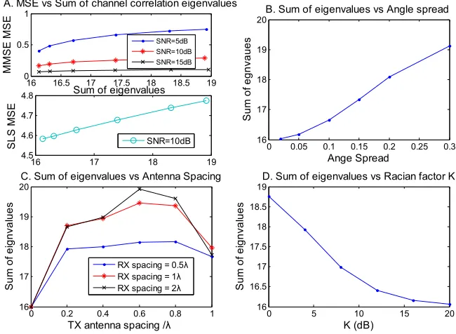
Figure 2 shows a relationship between MSE and the sum of eigenvalues of the channel correlation matrix for both MMSE and SLS methods. The results include an effect of maximum angle spread (AS), antenna spacing and Rician factor K, which are related to the sum of ei-genvalues of RH. The obtained results are given in four sub-figures A, B, C and D.

Sub-figure A supports the theory presented in Section 3 that for MMSE and SLS methods channel estimation errors are smaller for smaller sums of eigenvalues of RH. When the sum of eignvalues increases, the channel esti-mation accuracy becomes worse.

(6)

nd the MS transmitter antenna spacing. O

um of ei-ge

improve the accuracy of the training based MIMO chan-nel estimation.

Sub-figure C presents the relationship between the sum of eigenvalues a

Figure 3 is plotted in three dimensions (3D) to provide a further support for the results of Figure 2. In this figure, the relationship between MSE, TPNR ρ and K for MMSE method is presented at three different values of maximum AS (indicating three special correlation levels). One can see that when TPNR is increased to 30dB the estimation error decreases almost to zero. When the value of Rician factor K is increased, indicating a stronger LOS component in comparison with NLOS components, the MSE decreases. This is consistent with the trend observed in Figure 2 that a stronger LOS com-ponent results in better estimation accuracy.

ne can see that the sum of eigenvalues becomes smaller when the spacing distance is less than 0.2λ.

Sub-figure D gives the relationship between the sum of eigenvalues and the Rician factor K. The s

nvalues is smaller at higher values of K (when the LOS component is strongest). This means that a stronger LOS component reduces the sum of eigenvalues and thus improves the channel estimation accuracy.

0 0.05 0.1 0.15 0.2 0.25 0.3

16 17 18 19

20B. Sum of eigenvalues vs Angle spread

Ange Spread

Sum

of

egn

va

ues

0 5 10 15 20

16 16.5 17 17.5 18 18.5

19D. Sum of eigenvalues vs Racian factor K

K (dB)

S

u

m

of

ei

gn

va

lues

0 0.2 0.4 0.6 0.8 1

16 17 18 19

20C. Sum of eigenvalues vs Antenna Spacing

TX antenna spacing /λ

S

u

m

of

ei

gn

va

lues

RX spacing = 0.5λ

RX spacing = 1λ

RX spacing = 2λ

16 17 18 19

4.5 4.6 4.7 4.8

SLS

M

S

E

SNR=10dB

16 16.5 17 17.5 18 18.5 19

0 0.5 1

A. MSE vs Sum of channel correlation eigenvalues

Sum of eigenvalues

MM

S

E

MS

E

[image:6.595.136.461.234.472.2]

SNR=5dB SNR=10dB SNR=15dB

Figure 2. Relationship between MSE vs Sum of eigenvalues of RH showing an

im-pact of antenna spacing and the Rician factor K.

0

10 20

5 10 15 20 25 300 0.1 0.2 0.3 0.4 0.5 0.6 0.7

K (dB) MMSE of 4x4 MIMO MSE vs ρ vs K vs AS

ρ (dB)

MS

E

0.1 0.2 0.3 0.4 0.5 0.6 0.7

Angle Spread 0.2 rads

[image:6.595.179.418.511.698.2]

(7)

The presented results also show that for MMSE method MSE is reduced for the smallest AS, which cor-responds to the highest level of spatial correlation.

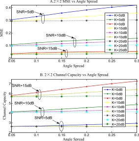
In the next step, we simulate the MIMO channel ca-pacity under the condition of channel estimation error. Simulations are run for the cases of 2×2 MIMO and 4x4 MIMO systems. The simulation settings including the distance between the transmitter and receiver, training sequence length, AoA, AS and antenna element spacing are same as in the earlier undertaken simulations. The minimum mean square error (MMSE) channel estimation method is applied for the Jakes model representing the channel between the BS and MS. The channel capacity is determined using Equation (40). For simulation purposes, RH is obtained using the actual channel matrix H and TPNR is assumed to be equal to SNR. 100000 channel realizations are used to obtain the value of capacity.

4 shows the resu

figure B.

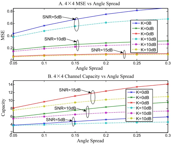
From Figure 4, one can see that the mean square error increases as the angle spread becomes larger. For all three groups, at K factor of 20dB, MSE shows the best performance while the worst accuracy occurs at the K factor of 0dB. In sub-figure B, the relationship trends are different from the ones observed in sub-figure A. As the angle spread increases, the channel capacity is enhanced. In all three groups of lines at three SNR values, the high-est capacity occurs at K equal to 0dB while at 20dB the capacity is decreased. These two sub-figures indicate that the channel capacity is increased when the channel esti-mation accuracy is reduced. This finding is opposite to the one shown in [26,27,29]. This could be due to the fact that in [26,27,29] the influence of spatial correlation or K factor on the channel capacity was not considered. The presented simulation results strengthen the notion tronger LOS estimation

ac-MO

ure lts for the 2×2 MIMO system.

s are plotted in two-dimensions (2D) that the higher spatial correlation (due to a scomponent) helps to improve the channel Simulation result

and include two sub-figures. Sub-figure A presents the relationship between MSE and angle spread (AS). There are three groups of lines drawn for three different values of SNR. In each group, the lines correspond to three dif-ferent values of K factor. The relationship between channel capacity and the angle spread is given in sub-

curacy. At the same time it decreases the rank and EDOF of the channel matrix.

[image:7.595.146.429.403.690.2]

Similar findings are obtained for the 4×4 MIMO sys-tem, as illustrated in Figure 5. The results are shown for SNR of 5, 10 and 15dB and the Rician factor K of 0 and 10dB.

Figure 4. MSE vs Angle Spread and Channel estimation vs Angle Spread of a 2×2 MI under 3 different SNR and 3 different K factor.

0.052 0.1 0.15 0.2 0.25 0.3 3

4 5 6 7

B. 2x2 Channel Capacity vs Angle Spread

Angle Spread

C

ha

nnel

C

apac

ity

0.050 0.1 0.15 0.2 0.25 0.3 0.1

0.2 0.3 0.4

A. 2x2 MSE vs Angle Spread

Angle Spread

MS

E

K=0dB K=0dB K=0dB K=10dB K=10dB K=10dB K=20dB K=20dB K=20dB

SNR=10dB

SNR=15dB SNR=5dB

SNR=15dB

A.2×2 MSE vs Angle Spread

MSE

Angle Spread

B. 2×2 Channel Capacity vs Angle Spread

Channel Capacity SNR=5dB

(8)

At K factor of while the wors As the angle sp creased. Th while at 10dB th

6. Conclusions

In this paper, the channel estimat capacity has bee analysis and sim accuracy of the tion is governed channel correlati to noise ratio (TPNR Specifically, a s more accurate channel

atial correlation (that o

is because the becomes reduced. The undertaken

ntenna Gaussian Telecommunications, vember 1999.

wald, “Capacity of a mo-unication link in Rayleigh

Information Theory, y 1999.

ott, and G. W. Wornell, tion in multiple-antenna annels,” IEEE Journal on

, No. 8, pp.

el estimation for space- EEE Transactions on Sig-15-2528, October 2002. At K factor of

while the wors As the angle sp creased. Th while at 10dB th

6. Conclusions

In this paper, the channel estimat capacity has bee analysis and sim accuracy of the tion is governed channel correlati to noise ratio (TPNR Specifically, a s more accurate channel

atial correlation (that o

is because the becomes reduced. The undertaken

ntenna Gaussian Telecommunications, vember 1999.

wald, “Capacity of a mo-unication link in Rayleigh

Information Theory, y 1999.

ott, and G. W. Wornell, tion in multiple-antenna annels,” IEEE Journal on

, No. 8, pp.

el estimation for space- EEE Transactions on Sig-15-2528, October 2002.

[image:8.595.151.428.85.320.2]

A. 4x4 MSE v ngle Spread

Figure 5. MSE vs Angle Spread and Channel estimation vs Angle

read of a 4×4 MIMO under 3 different SNR and 3 different K factor.

10dB, MSE shows the best performance t accuracy occurs at the K factor of 0dB. read increases, the channel capacity in-e highin-est capacity occurs at K in-equal to 0dB

e capacity is decreased.

effect of spatial correlation on MIMO ion accuracy and the resulting channel n i stigated. The mathematical ulation results have shown that the training based MIMO channel

by the sum of eigenvalues of the on matrix when the transmitted power

) in the training mode is fixed. maller

7. References

[1] E. Telatar, “Capacity of multi-a nels,” European Transactions on

. 6, pp. 585- 596, No [2] T. L. Marzetta and B. M. Hoch

bile multiple-antenna comm flat fading,” IEEE Transactions on Vol. 45, No. 1, pp. 139-157, Januar [3] A. Narula, M. J. Lopez, M. D. Tr

“Efficient use of side informa data transmission over fading ch

Selected Areas in Communications, Vol. 16 1423-1436, October 1998.

[4] C. Budianu and L. Tong, “Chann

ead of a 4×4 MIMO under 3 different SNR and 3 different K factor.

10dB, MSE shows the best performance t accuracy occurs at the K factor of 0dB. read increases, the channel capacity in-e highin-est capacity occurs at K in-equal to 0dB

e capacity is decreased.

effect of spatial correlation on MIMO ion accuracy and the resulting channel n i stigated. The mathematical ulation results have shown that the training based MIMO channel

by the sum of eigenvalues of the on matrix when the transmitted power

) in the training mode is fixed. maller

7. References

[1] E. Telatar, “Capacity of multi-a nels,” European Transactions on

. 6, pp. 585- 596, No [2] T. L. Marzetta and B. M. Hoch

bile multiple-antenna comm flat fading,” IEEE Transactions on Vol. 45, No. 1, pp. 139-157, Januar [3] A. Narula, M. J. Lopez, M. D. Tr

“Efficient use of side informa data transmission over fading ch

Selected Areas in Communications, Vol. 16 1423-1436, October 1998.

[4] C. Budianu and L. Tong, “Chann

Sp

nve nve

sum of eigenvalues leads to a estimation. A higher level of is due to a stronger LOS

com-time orthogonal block codes,” I nal Processing, Vol. 50, pp. 25 sum of eigenvalues leads to a

estimation. A higher level of is due to a stronger LOS

com-time orthogonal block codes,” I nal Processing, Vol. 50, pp. 25 sp

p sp

p nent and smaller angle spread) leads to a reduced value of the sum of channel correlation eigenvalues and hence has a positive influence on the channel es-timation accuracy. However, this improvement in channel estimation does not necessarily lead to im-proving the channel capacity. This

nent and smaller angle spread) leads to a reduced value of the sum of channel correlation eigenvalues and hence has a positive influence on the channel es-timation accuracy. However, this improvement in channel estimation does not necessarily lead to im-proving the channel capacity. This

channel matrix rank channel matrix rank

computer simulations undertaken for the uplink case, in which a mobile station (MS) transmitter is sur-rounded by scattering objects, have shown that higher spatial correlation levels due to a stronger LOS com-ponent decrease MIMO channel capacity despite the fact that channel estimation accuracy is improved.

[5] A. Grant, “Joint decoding and channel estimation for linear MIMO channels,” Proceedings of IEEE Wireless Communications Networking Conference, Vol. 3, pp. 1009-1012, Chicago, IL, September 2000.

[6] A. S. Kyung, R. W. Heath, and B. K. Heung, “Shannon capacity and symbol error rate of space-time block codes in MIMO Rayleigh channels with channel estimation er-ror,” IEEE Transactions on Wireless Communication, Vol. 7, No. 1, pp. 324-333, January 2008.

[7] X. Zhang and B. Ottersten, “Performance analysis of V- BLAST structure with channel estimation errors,” IEEE 4th Workshop on Signal Processing Advances in Wire-less Communications SPAWC, pp. 487-491, June 2003. computer simulations undertaken for the uplink case,

in which a mobile station (MS) transmitter is sur-rounded by scattering objects, have shown that higher spatial correlation levels due to a stronger LOS com-ponent decrease MIMO channel capacity despite the fact that channel estimation accuracy is improved.

[5] A. Grant, “Joint decoding and channel estimation for linear MIMO channels,” Proceedings of IEEE Wireless Communications Networking Conference, Vol. 3, pp. 1009-1012, Chicago, IL, September 2000.

[6] A. S. Kyung, R. W. Heath, and B. K. Heung, “Shannon capacity and symbol error rate of space-time block codes in MIMO Rayleigh channels with channel estimation er-ror,” IEEE Transactions on Wireless Communication, Vol. 7, No. 1, pp. 324-333, January 2008.

[7] X. Zhang and B. Ottersten, “Performance analysis of V- BLAST structure with channel estimation errors,” IEEE 4th Workshop on Signal Processing Advances in Wire-less Communications SPAWC, pp. 487-491, June 2003.

s A

Vol. 10, No Vol. 10, No

0.050 0.1 0.15 0.2 0.25 0.3

0.2 0.4 0.6 0.8 Angle Spread MS E

A. 4×4 MSE v ead

0.052 0.1 0.15 0.2 0.25 0.3

4 6 8 10 12 14

B. 4x4 Channel Capacity vs Angle Spread

Angle Spr apac ity ead C K=0B K=0dB K=0dB K=10dB K=10dB K=10dB K=0dB K=0dB K=0dB K=10dB K=10dB K=10dB SNR=5dB SNR=5dB SNR=10dB SNR=10dB S

s Angle Spr

MSE

NR=15dB

Angle Spread

B. 4×4 Channel Capacity vs Angle Spread

SNR=15dB

Capacity

(9)

een

Communications, ICC’04, Paris, France, Vol. 5, pp. 2658-2662, June 2004.

n Signal

oceedin

dings of IEEE International

pproximation

eless channels:

ansakul, M. E. Bialkowski, S. Durrani, K.

Bi-EEE International Antennas Propagation

for antenna arrays incorporating

azi-n liazi-nk iazi-n Rayleigh flat

. 5, pp. 2203-2214, May 2006.

ence on Communications, Vol. 2, pp. 808-

sactions on Information

S. Aissa, “On the per-[8] P. Layec, P. Piantanida, R. Visoz and A. O. Berthet,

“Capacity bounds for MIMO multiple access channel with imperfect channel state information,” IEEE In-formation Theory Workshop ITW08, pp. 21-25, May 2008.

[9] M. Biguesh and A. B. Gershman, “MIMO channel estimation: Optimal training and tradeoffs betw

niques,” Proceedings of Internation

Symp

estimation tech Conference on

al _[

[10] M. Biguesh and A. B. Gershman, “Training-based MIMO channel estimation: A study of estimator tradeoffs and optimal training signals,” IEEE Transactions o

Processing, Vol. 54, No. 3, pp. 884-893, March 2006. [11] X. Liu, S. Lu, M. E. Bialkowski and H. T. Hui, “MMSE

Channel estimation for MIMO system with receiver

equipped with a circular array antenna,” Pr gs of muth spread,” IEEE Transactions on Vehicular Technol-_{ogy, Vol. 51, No. 5, pp. 968}_-_{977, September 2002.} [23] S. M. Kay, “Fundamentals of statistic signal processing:

Estimation theory”, Prentice-Hall, Inc., 1993. IEEE Microwave Conference APMC2007, pp. 1-4,

De-cember 2007.

[12] X. Liu, M. E. Bialkowski, and S. Lu, “Investigation into training-based MIMO channel estimation for spatial cor-relation channels,” Procee

Antennas Propagation Symposium (APS-2007), pp. 51-55, August 2007.

[13] P. B. Rapajic and D. Popescu, “Information capacity of a [2 random signature multiple-input multiple-output chan-nel,” IEEE Transactions on Communications,Vol. 48, pp. 1245-1248, August 2000.

[14] P. J. Smith and M. Shafi, “On a Gaussian a

to the capacity of wireless MIMO systems,” Proceedings of International Conference on Communications, ICC’02, pp. 406-410, 2002.

[15] P. F. Driessen and G. J. Foschini, “On the capacity for-mula for multiple-input multiple-output wir

A geometric interpretation,” IEEE Transactions on Com-munications, Vol. 47, pp. 173-176, February 1999. [16] D. Shiu, G. J. Foschini, M. J. Gans, and J. M. Kahn,

“Fading correlation and its effect on the capacity of mul-tielement antenna systems,”IEEE Transactions on Com-munications, Vol. 48, No. 3, pp. 502-513, March 2000. [17] V. Erceg, “Indoor MIMO WLAN channel models,” IEEE

802.11-03/161r2, September 2003. [18] P. Uth

form

alkowski, and A. Postula, “Effect of line of sight

propa-gation on capacity of an indoor MIMO system,” Pro-ceedings of I

osium (APS-2005), Washington, DC, pp. 707-710, 2005.

[19] E. G. Larsson and P. Stoica, “Space-time block coding for wireless communication,” Cambridge University Press, 2003.

20] C. N. Chuah, D. N. C. Tse, and J. M. Kahn, “Capacity scaling in MIMO wireless systems under correlated fad-ing,” IEEE Transactions on Information Theory, Vol. 48, pp. 637-650, March 2002.

[21] W. C. Jakes, “Microwave mobile communications,” New York: John Wiley & Sons, 1974.

[22] T. L. Fulghum, K. J. Molnar and A. Duel-Hallen, “The Jakes fading model

[24] G. J. Foschini and M. J. Gans, “On the limits of wireless communications in fading environment when using mul-tiple antennas,” Wireless Personal Communications, Vol. 6, pp. 311-335, 1998.

5] B. M. Hochwald and T. L. Marzetta, “Capacity of a mo-bile multiple antenna communicatio

fading,” IEEE Transactions on Information Theory, Vol. 45, No. 1, pp. 139-157, January 1999.

[26] T. Yoo and A. Goldsmith, “Capacity and power alloca-tion for fading MIMO channels with channel estimaalloca-tion error,” IEEE Transactions on Information Theory, Vol. 52, No

[27] T. Yoo and A. Goldsmith, “Capacity of fading MIMO channels with channel estimation error,” IEEE Interna-tional Confer

813, June 2004.

[28] M. Medard, “The effect upon channel capacity in wire-less communications of perfect and imperfect knowledge of the channel,” IEEE Tran

ory, Vol. 46, pp. 933-946, May 2000. [29] M. Torabi, M. R. Soleymani, and