Bayesian model choice via mixture distributions
with application to epidemics and population
process models
Philip D. O’Neill1,
Theodore Kypraios1
1School of Mathematical Sciences, University of Nottingham, UK
Abstract
We consider Bayesian model choice for the setting where the observed data are partially observed realisations of a stochastic population process. A new method for computing Bayes factors is described which avoids the need to use reversible jump approaches. The key idea is to perform infer-ence for a hypermodel in which the competing models are components of a mixture distribution. The method itself has fairly general applicability. The methods are illustrated using simple population process models and stochastic epidemics.
Keywords: Bayes factors; Epidemic models; Markov chain Monte Carlo meth-ods; Model choice
1
Introduction
Consider an observed sequence of event times, each event being of the same type,
and suppose we wish to assess whether a homogeneous Poisson process or an
al-ternative non-homogeneous Poisson process best fits the observations.
and wish to know which of two possible SIR (susceptible-infective-removed)
dis-ease transmission models is most plausible as a model for how the data were
generated, assuming that removals correspond to case-detections. Both of these
examples are special cases of a generic situation in which we wish to assess which
of a number of proposed point-process models best fits the data to hand. In
the first example there is one type of event, and all events are observed. In the
second example there are two event types (infections and removals) but only the
latter are observed. In both examples two models are compared, but in general
we may have more models of interest.
In a Bayesian framework, questions of model choice can be addressed using
Bayes factors, which quantify the relative likelihood of any two models given
the data and within-model prior distributions. Bayes factors can suffer from
two practical drawbacks, namely (i) they can be difficult to compute, and (ii)
they can be highly sensitive to the choice of within-model prior distributions,
and in particular apparently natural choices can give misleading results. Here
our focus is towards addressing the first difficulty, but in respect of the second
we briefly remark that alternative methods of Bayesian model assessment have
their own difficulties in the setting we consider. For example, neither the
De-viance Information Criteron (DIC) nor Bayesian Information Criterion (BIC)
appear entirely natural for settings where the data are typically far from
be-ing independent observations, as is the case when the data are realisations of a
stochastic process. For problems involving missing data, such as the epidemic
example above, it is not even clear how suitable information criteria should best
be defined (Celeux et al. (2006) give nine candidates, for instance). Finally,
methods involving a comparison between the observed data and what the fitted
model would predict typically involve a subjective judgement as to precisely
what should be compared, and how.
In all but the simplest cases, Bayes factors must be evaluated numerically.
For many problems, this can be achieved via reversible jump Markov chain
Monte Carlo (RJMCMC) methods (Green, 1995). To be precise, consider two
Define k ∈ {1,2} to be a model indicator which specifies the model under consideration. RJMCMC methods proceed by defining a Markov chain with
state space {1} ×Θ1∪ {2} ×Θ2 such that the proportion of time for which
k=j converges to the posterior model probabilityP(Mj|x), where xdenotes the observed data. Given model prior probabilitiesP(Mj), the Bayes factor in
favour of model 1 is given by the expressionP(M2)P(M1|x)/P(M1)P(M2|x),
which can be estimated from the RJMCMC output.
The main practical challenge in implementing RJMCMC algorithms is
con-structing efficient between-model proposal distributions, i.e. defining how the
Markov chain jumps between the different components of the union of model
parameter spaces. Although there have been theoretical advances which address
this issue (Brooks et al., 2003), for many problems it remains a case of trial and
error. In this paper we propose a method which goes some way to removing
this complication. The key idea is to consider a hypermodel which is itself a
mixture model whose components are the two or more competing models of
interest. An MCMC algorithm can then be defined on the product space of all
model parameters and mixture probabilities. Bayes factors for the models can
be expressed in terms of the posterior means of the mixture probabilities, and
thus estimated from the MCMC output.
Before proceeding to the details, we consider the general context. First,
defining a Markov chain on a product (rather than union) of model-parameter
spaces is the approach pioneered by Carlin and Chib (1995), and further
devel-oped to more general settings (Green and O’Hagan (1998), Dellaportas et al.
(2002), Godsill (2001)). This approach, as for RJMCMC, involves defining a
probability distribution over the set of possible models, and introduces a
param-eter which indicates which model is chosen. In our setting there is no chosen
model as such, but instead a mixture of all possible models. The product-space
approach also relies on defining so-called pseudo-priors for the within-model
parameters, upon which algorithm efficiency is crucially dependent, and this
can be difficult in practice. Our methods do not involve the need to introduce
similar prior distributions for the missing data.
Second, computational methods for the Bayesian analysis of mixture models
are well-established, both when the number of components in the mixture is
known (Diebolt and Robert, 1994) and when it is not (Richardson and Green,
1997). The typical situation under consideration is one in which the data are
assumed to comprise independent and identically distributed observations from
the proposed mixture distribution(s). In contrast, we consider the case where
there is only one datum, but it consists of the realisation of a stochastic process,
either fully or partially observed.
The paper is structured as follows. Section 2 contains general theory which
describes the inference framework in detail, and computational matters are
de-scribed in Section 3. Section 4 contains examples and we conclude with
discus-sion in Section 5.
2
General Theory
In this section we introduce the underlying framework of interest. For ease of
exposition we adopt the usual abuse of notation and terminology in which ‘a
densityπ(θ)’ can refer to both the density function π of a random variable θ,
or the same function evaluated at a typical pointθ.
2.1
Mixture model with no missing data
Suppose we observe datax, and wish to considerncompeting modelsM1, . . . , Mn.
Fori= 1, . . . , n denote the probability density ofxunder model ibyπi(x|θi), whereθidenotes the vector of within-model parameters, and setθ= (θ1, . . . , θn). We assume that all theπi(x|θi) are densities with respect to the same common reference measure. Define a mixture model by
π(x|α, θ) = n
∑
i=1
αiπi(x|θi), (1) whereα= (α1, . . . , αn) satisfies
∑n
2.2
Mixture model with missing data
In our setting, the dataxmay be a partial observation of a stochastic process.
In consequence,πi(x|θi) in (1) may be intractable, meaning that it cannot be analytically or numerically evaluated in an efficient manner. We adopt data
augmentation to overcome this problem, as follows. Let y = (y1, . . . , yN) be a vector comprising different kinds of ‘missing data’, and for i = 1, . . . , n let
I(i)⊆ {1, . . . , N} and defineyI(i) as the vector with componentsyj, j∈ I(i).
ThusyI(i) denotes the missing data for modeli, and in practice it is chosen to
make the augmented probability densityπi(x, yI(i)|θi) tractable. If modelidoes
not require missing data, thenyI(i) is null. Note that this formulation allows
different models to share common elements of missing data. Conversely, if each
model has its own missing data then we simply setI(i) =ifori= 1, . . . , n. In order to define a mixture model using missing data, it is necessary to
introduce additional terms so that each component of the mixture is a
probabil-ity densprobabil-ity function on the possible values ofxandy. To this end, we assume
that there exist tractable probability densitiesπi(y−I(i)|x, yI(i), θ), wherey−I(i)
denotes the vector with componentsyj,j /∈ I(i). If the latter set is empty then we set πi(y−I(i)|x, yI(i), θ) = 1. We refer to the πi(y−I(i)|x, yI(i), θ) terms as missing data prior densities. In practice, they need not explicitly depend on any ofx, yI(i) orθ, depending on the application at hand.
Define an augmented mixture model by
π(x, y|α, θ) = n
∑
i=1
αiπi(x, yI(i)|θi)πi(y−I(i)|x, yI(i), θ). (2)
Here we assume that eachπi(x, yI(i)|θi)πi(y−I(i)|x, yI(i), θ) term in the sum in
(2) is a probability density with respect to a common reference measure, from
which it follows thatπ(x, y|α, θ) is also a probability density.
2.3
Bayes Factors
We now show how Bayes factors can be computed directly from certain
assume thatα,θ1, . . . ,θn are mutually independenta priori. By Bayes’ Theo-rem,
π(α|x) =π(x|α)π(α)
π(x) =
π(α)∑ni=1αimi(x)
π(x) ,
whereπ(α) denotes the prior density ofαand, fori= 1, . . . , n,
mi(x) =
∫
πi(x, yI(i)|θi)πi(θi)dθidyI(i),
whereπi(θi) is the within-model prior density ofθi. Note also that
1 =
∫
π(α|x)dα=π(x)−1 n
∑
i=1
E[αi]mi(x),
whence
π(x) = n
∑
i=1
E[αi]mi(x). (3)
Now fori̸=j, the Bayes factor in favour ofMi relative toMj is defined to beBij =Bij(x) =mi(x)/mj(x). However,
E[αi|x] =
∫
αiπ(α|x)dα = π(x)−1
∫
αi
∑n
j=1
αjmj(x)
π(α)dα
= π(x)−1 n
∑
j=1
E[αiαj]mj(x),
which combined with (3) yields that
E[αi|x] =
∑n
j=1E[αiαj]mj(x)
∑n
j=1E[αj]mj(x)
, i= 1, . . . , n. (4)
Next, fixk∈ {1, . . . , n}. Dividing the numerator and denominator of the frac-tion in (4) bymk(x) and rearranging we obtain
n
∑
j=1
(E[αj]E[αi|x]−E[αiαj])Bjk(x) = 0, i= 1, . . . , n. (5) It remains to solve equations (5) to find Bjk(x), j = 1, . . . , n. DefineA as
then×nmatrix with elements
Note thatAdepends onx, although we suppress this dependence in our
nota-tion. Define ˜A−kas the (n−1)×(n−1) matrix formed by removing thekth row andkth column ofA. Similarly for j̸=k define ˜A−jk as the (n−1)×(n−1) matrix formed from ˜A−kby replacing the elementsAij with−Aik,i= 1, . . . , n,
i̸=k.
Lemma 1. (a) If det ˜A−k ̸= 0 then
Bjk(x) =
det ˜A−jk
det ˜A−k
. (6)
(b) Suppose that 0< mi(x)<∞fori= 1, . . . , n. Then if either (i)n= 2 and 0< E[α1]<1, or (ii)αhas a Dirichlet prior distribution,D(p1, . . . , pn), then
Bjk(x) =Ajk
Akj
.
The proof of Lemma 1 is in the Appendix. The result shows that the required
Bayes factors can be expressed in terms of the prior distribution summariesE[αi]
andE[αiαj] and the posterior meansE[αi|x],i, j= 1, . . . , n.
The condition on the determinant of ˜A−k in Lemma 1(a) is not vacuous in
general, as illustrated by the somewhat pathological case whereαi has a point
mass prior for alli= 1, . . . , n. Then for all 1≤i, j ≤n, E[αi|x] =E[αi] and
E[αiαj] = E[αi]E[αj], whence Aij = 0 and (5) cannot be solved to find the
Bayes factors.
At first sight the need for a Dirichlet prior onαto yield simple evaluation of
the Bayes factors via Lemma 1 may appear restrictive. We make three remarks.
First, the mixture construction is itself introduced solely as a tool for evaluation
of Bayes factors, and so there is no particular need to assign an arbitrary prior
distribution toα. Second, in practice a Dirichlet prior is both straightforward to
use and flexible enough for computational purposes as described below. Third,
it may well be that (6) holds for arbitrary prior distributions on α, subject
Finally, the simple form for the Bayes factor in Lemma 1 (b) does not appear
to be true in general; an example forn= 3 can be found in the Appendix.
2.4
Two competing models
We give special attention to the casen= 2 since this is of practical importance.
Here we haveα= (α1,1−α1) and Lemma 1 yields that
B12=
E[α1]−E[α21]−E[α1|x](1−E[α1])
E[α1]E[α1|x]−E[α21]
.
It follows that
E[α1]−E[α21]
1−E[α1]
≤E[α1|x]≤
E[α2 1]
E[α1]
,
with the upper and lower bounds corresponding to Bayes factors entirely in
favour of models 1 and 2, respectively. A practical consequence is that any
numerical estimate ofE[α1|x] lying outside these bounds must be incorrect.
Under the further assumption thatπ(α) is a uniform density, so thatα1 ∼
U(0,1), we obtain
B12=
3E[α1|x]−1
2−3E[α1|x]
,
π(α1|x)∝α1m1(x) + (1−α1)m2(x),
E[α1|x] = (2m1(x) +m2(x))/(3(m1(x) +m2(x)) and 1/3≤E[α1|x]≤2/3.
Finally, ifαis assigned a Dirichlet prior distribution, bounds forE[αi|x] for any value ofncan be obtained. Full details can be found in the proof of Lemma
1 in the Appendix.
3
Computation
We now describe how to use the mixture framework in practice, specifically via
MCMC methods. Our objective is to sample from the target density
π(α, θ, y|x)∝π(x, y|α, θ)π(α)π(θ), (7) and the first issue is that of assigning any missing data prior density terms in
3.1
Missing data prior densities
Although the desired Bayes factors are invariant to the choice of any missing
data prior densities, this choice is important in practice for computations. This
is largely a problem-specific issue, but we make two general remarks. First, if
all models share the same missing data (y1, say) then no missing data prior
densities are required, and (7) becomes
π(α, θ, y|x)∝ n
∑
i=1
αiπi(x, y1|θi)π(α)π(θ).
Second, it can be beneficial to assign missing data priors which mimic the
marginal density of they−I(i)components in other models. As discussed below,
the mixing properties of suitable MCMC algorithms are improved if the chains
can easily move between different models, and such movement is hindered if the
density of the missing data in one model is very different to the missing prior
density assigned in another.
3.2
MCMC methods
Sampling from the target density defined at (7) will typically be possible via
a range of standard MCMC methods, but here we offer some observations on
practical aspects. The fact that the target density is a sum will usually make
direct Gibbs sampling infeasible, but the approach of Diebolt and Robert (1994),
which relies on the introduction of allocation variables which indicate the ‘true’
model as described in Dempster et al. (1977), can be adapted as follows.
Introduce z = (z1, . . . , zn) such that zi ∈ {0,1} and
∑n
i=1zi = 1. Thus z can takenpossible values, each of which is a vector of zeroes other than a 1 at
one position. Define the augmented likelihood
π(z, x, y|α, θ) = n
∏
i=1
(αiπi(x, yI(i)|θi)πi(y−I(i)|x, yI(i), θ))zi,
so that the augmented likelihood at (2) is recovered by summing over z. If
conditional distribution
α| · · · ∼ D(p1+z1, . . . , pn+zn).
The full conditional distribution ofzis multinomialM(1;q1, . . . , qn), where the
probabilities are given by
qi∝αiπi(x, yI(i)|θi)πi(y−I(i)|x, yI(i), θ), i= 1, . . . , n.
Fori= 1, . . . , n,θi has full conditional distribution given by
π(θi| · · ·)∝
πi(θi) zi= 0,
πi(x, yI(i)|θi)πi(θi) zi= 1.
Finally, any missing data component yj, j = 1, . . . , N, has full conditional
distribution given by
π(yj| · · ·)∝
πi(x, yI(i)|θi) j∈ I(i),
πi(y−I(i)|x, yI(i), θi) j /∈ I(i),
whereidenotes the current model, i.e. zi= 1.
The prior distribution forαcan often be chosen to improve the mixing of the
MCMC algorithm above. In particular this can be achieved by trying to make
the multinomial distribution ofz as close to uniform as possible. To illustrate
this, consider the trivial example with two models in which π1(x)/π2(x) =
m1(x)/m2(x) =B12= 50. The full conditional distributions for z1 andα1 are,
respectively,Bern(50α1/(50α1+ (1−α1))) andBeta(z1+p1,1−z1+p2), where
Bern and Beta respectively denote Bernoulli and Beta distributions. Setting
p1 =p2 = 1 produced wildly different estimates forB12 (87.8, 40.9, 547.1) for
three MCMC runs of 106 iterations, while repeating the exercise withp 1 = 1
andp2= 50 yielded estimates 50.3, 50.3 and 50.7.
It is of course not necessary to use allocation variables, and one can equally
use any suitable MCMC scheme for the target density. However, the above
illustrates the fact that the full conditional distributions ofθi and any missing
data will be of mixture form, which has implications for the design of efficient
are mixtures, and in particular are not the same as those obtained from a
single-model analysis, which are proportional toπi(x|θi)πi(θi). The marginal densities can be either be explored via a standard single-model MCMC algorithm, or by
using the allocation variables approach and conditioning the output onzi = 1
to obtain within-model posterior density samples forθi.
3.3
Connections with other approaches
The framework we adopt is related to that described in Carlin and Chib (1995)
and Godsill (2001), in which the target distribution of interest is defined over
a product space of models and their parameters. In order to clarify the
differ-ences in our approach, consider the simplest possible setting in which we have
two models defined by densitiesπ1(x|θ1) andπ2(x|θ2), and within-model prior
densities π1(θ1) and π2(θ2). The framework of Carlin and Chib (1995) and
Godsill (2001) introduces a model indicatork ∈ {1,2} to denote the ‘current’ model. The target density of interest is specified by
π(k, θ1, θ2|x)∝πk(x|θk)πk(θk|k)π(θ3−k|θk, k)π(k),
where it is necessary to specifyπ(θ3−k|θk, k), i.e. the ‘prior’ for the non-current model parameter. Assumingθ1 and θ2 to be independent of each other and k
gives thatπ(θ3−k|θk, k) =π3−k(θ3−k).
Conversely, our formulation has target density
π(α, θ1, θ2|x)∝π(α)π1(θ1)π2(θ2)[α1π1(x|θ1) +α2π2(x|θ2)].
If we adopt the allocation-variable approach, the target density becomes
π(z, α, θ1, θ2|x)∝π(α)π1(θ1)π2(θ2)[α1π1(x|θ1)]z1[α2π2(x|θ1)]z2,
from which we see that it is the existence of theαparameter which distinguishes
our formulation from that of Carlin and Chib (1995) and Godsill (2001). Of
course, posterior estimation ofα is what enables us to estimate Bayes factors,
The general formulation in Godsill (2001) also allows each model to
poten-tially share parameters with other models. Specifically, the parameters of model
kwill be some subset of a set of parameters{θ1, . . . , θN}. This is similar to the way we have dealt with missing data, although the two set-ups are not
tech-nically equivalent, and in particular one cannot simply treat our missing data
as model parameters. The fundamental difference is that missing data may not
always require a prior, whereas model parameters always do. For instance, if a
densityπ(x|θ) is intractable, then our missing data approach uses Bayes’ Theo-rem in the formπ(θ, y|x)∝π(x, y|θ)π(θ) whereas augmenting with extra model parameterψgivesπ(θ, ψ|x)∝π(x|θ, ψ)π(θ, ψ).
4
Examples
In this section we illustrate the theory with three examples featuring
popu-lation processes or epidemics. First, however, we consider a simpler classical
example which briefly compares our methods with alternatives. This example
illustrates that our methods have wider applicability than population processes,
and moreover appear to be competitive against alternative methods.
4.1
Pines data
We consider the well-known model choice problem of assigning non-nested linear
regression models to the pines data set in Williams (1959). These data have been
analyzed by several authors (see, for example, Han and Carlin, 2001; Carlin and
Chib, 1995; Friel and Pettitt, 2008) in order to compare methods for estimating
Bayes factors. The data describe the maximum compression strength parallel to
the grainyi, the densityxi, and the resin-adjusted density zi for 42 specimens
of radiata pine. The two competing models we consider are
M1: yi=α+β(xi−x¯) +ϵi, ϵi∼N(0, σ2);
Table 1: Pines data set: Comparison of Bayes factors from different methods
Method Bias Standard Error
RJMCMC 67 2678
RJ corrected 9 124
Power posterior (serial MCMC) 10 132
Power posterior (population MCMC) 22 154
Mixture method 10 39
We assigned identical prior distributions for the parametersα, β, γ, δ, σ2 andτ2
as the papers cited above. We assigned a Beta(100,1) prior distribution for
α1 and carried out 100 MCMC runs of our method, this being the same as
the number of MCMC runs used for the methods described in Friel and Pettitt
(2008).
Furthermore, Friel and Pettitt (2008) compared conventional RJMCMC
methods (with each modela prioriequally likely), ‘corrected’ RJMCMC meth-ods (model priors chosen to improve mixing) and two power posterior methmeth-ods
(Serial and Population MCMC). Full details can be found in Friel and Pettitt
(2008), and for convenience we simply quote the results obtained in Table 1,
along with our result. The bias is calculated by comparison with the estimate
of 4862 obtained by numerical integration in Green and O’Hagan (1998). It can
be seen that our method is certainly competitive.
4.2
Poisson process vs. linear birth process
Our first population process example is analytically tractable and illustrates that
our methods produce results in agreement with the known true values. Consider
data given by the vector of event timesx= (x1, . . . , xn) observed during a time
interval [0, T], where 0≤x1≤x2≤. . .≤xn ≤T. We will compare two models, namely a homogeneous Poisson process of rateλ(M1) and a linear birth process
{X(t) :t∈[0, T]} with per-capita birth rate µ and X(0) = 1 (M2). Suppose
with meanθ−1. The model likelihoods, which we write as densities with respect to the reference measure induced by a unit rate Poisson process on [0, T], are
π1(x|λ) =λnexp{−(λ−1)T}, π2(x|µ) =n!µnexp{−µ[(n+ 1)T −S(x)] +T},
whereS(x) =∑nj=1xj. In this setting no missing data are required so we use the model defined at (1). The Bayes factor in favour ofM1 relative toM2 is
B12= ∫
π1(x|λ)π(λ)dλ ∫
π2(x|µ)π(µ)dµ
=
∫∞ 0 θλ
nexp{−λ(T+θ)} dλ
∫∞ 0 θn!µ
nexp{−µ[(n+ 1)T−S(x) +θ]} dµ = [(n+ 1)T−S(x) +θ]
n+1
(T+θ)n+1n! .
Assuming that α1 ∼ U(0,1) a priori, a simple Gibbs sampler for the target
density consists of parameter updates as follows:
α1| · · · ∼ Beta(z1+ 1,2−z1),
z1| · · · ∼ Bern (
α1π1(x|λ)
α1π1(x|λ) + (1−α1)π2(x|µ) )
,
λ| · · · ∼
Γ(1, θ) z1= 0,
Γ(n+ 1, T +θ) z1= 1,
µ| · · · ∼
Γ(n+ 1,(n+ 1)T−S(x) +θ) z1= 0,
Γ(1, θ) z1= 1,
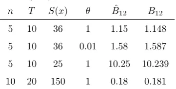
where Γ(m, ξ) denotes a Gamma distribution with densityf(x)∝xm−1exp(−ξx). Typical results from MCMC runs are given in Table 2, illustrating that the
Gibbs sampler recovers the true known values. We found that the algorithm
mixing was good in all cases.
Finally, we comment on the relationship between the above algorithm and
standard reversible jump methods. The RJMCMC requires a way of proposing
a value of µ given λ for jumps from M1 to M2, and vice versa. In practice
it is not immediately obvious how best to do this, but an approach suggested
in Green (2003) is to propose µ independently of λ, ideally according to the
Table 2: Example 2: Bayes factors from MCMC output ( ˆB12) compared to true
values (B12).
n T S(x) θ Bˆ12 B12
5 10 36 1 1.15 1.148
5 10 36 0.01 1.58 1.587
5 10 25 1 10.25 10.239
10 20 150 1 0.18 0.181
4.3
SIR model with two different infection periods
Recall the standard SIR (Susceptible-Infective-Removed) epidemic model (see
e.g. Andersson and Britton (2000), Chapter 2), defined as follows. A closed
population containsN+aindividuals of whomN are initially susceptible and
ainitially infective. Each infective remains so for a period of time distributed
according to a specified random variableTI, known as the infectious period, after
which it becomes removed and plays no further part in the epidemic. During
its infectious period an infective makes contact with each other member of the
population at times given by a homogeneous Poisson process of rateβ/N, and
any contact occurring with a susceptible individual results in that individual
immediately becoming infective. The infectious periods of different individuals
and the Poisson processes between different pairs of individuals are assumed to
be mutually independent. The epidemic ends when there are no infectives left
in the population.
A distinguishing characteristic of infectious disease data is that the infection
process itself is rarely observed, and so we suppose that the datar consist of
nobserved removal times r1 ≤. . . ≤rn. We consider two competing models,
namely that TI ∼ Γ(1, γ) (M1) and TI ∼Γ(m, λ) (M2), where the shape
pa-rametermwill be assumed known. Both model likelihoodsπ1(r|γ) andπ2(r|λ)
are intractable in practice since their evaluation relies on integrating over all
possible realisations of the infection process, and so we introduce missing data
Forj= 1, . . . , n defineij as the infection time of the individual removed at
timerj. We assume that there isa= 1 initial infective, denoted byp, so that
ip≤ijfor allj̸=p. For simplicity we assumea priorithatpis equally likely to be any of theninfected individuals and thatip has an improper uniform prior
density on (−∞, r1). Finally, definei={ij :i̸=p} to be then−1 non-initial infection times. Fork= 1,2 the augmented model likelihoods, which we write
here with respect to Lebesgue measure onR2n−1, are
πk(i, r|p, ip, βk, ηk) =
∏n
j=1;j̸=p
(βk/N)I(ij−)
exp
{
−(βk/N)
∫ rn
ip
S(t)I(t)dt
} ∏n
j=1
fk(rj−ij|ηk)
,
whereS(t) and I(t) denote respectively the numbers of susceptibles and
infec-tives at timet,I(t−) = lims↑tI(s), βk denotes the parameterβ under Mk, fk denotes the infectious period density under Mk, η1 = γ and η2 = λ (see e.g.
O’Neill and Roberts (1999), Streftaris and Gibson (2004), H¨ohle and O’Neill
(2005)). Note that in this formulation, the missing datai,pandipare assumed
common to both models, although these quantities could also be model-specific.
The target density of interest is
π(α1, β1, β2, γ, λ|r)∝[α1π1(i, r|p, ip, β1, γ)+(1−α1)π2(i, r|p, ip, β2, λ)]π(β1)π(β2)π(γ)π(λ).
Note that here we need no missing data priors densities because the the missing
data appear in both model likelihoods. Prior distributions for β1, β2, γ and λ
were all set as Γ(1,1), andα1∼Beta(p1, p2).
below, each of which yields a simple Gibbs update for the parameter in question.
α1| · · · ∼ Beta(z1+p1,1−z1+p2),
z1| · · · ∼ Bern (
α1π1(i, r|p, ip, β1, γ)
α1π1(i, r|p, ip, β1, γ) + (1−α1)π2(i, r|p, ip, β2, λ) )
,
β1| · · · ∼
Γ(n, N−1∫rn
ip S(t)I(t)dt+ 1) z1= 0,
Γ(1,10−3) z1= 1,
β2| · · · ∼
Γ(1,1) z1= 0,
Γ(n, N−1∫rn
ip S(t)I(t)dt+ 1) z1= 1,
γ| · · · ∼
Γ(n+ 1,∑nj=1(rj−ij) + 1) z1= 0,
Γ(1,1) z1= 1,
λ| · · · ∼
Γ(1,1) z1= 0,
Γ(nm+ 1,∑nj=1(rj−ij) + 1) z1= 1,
Finally, the infection time parametersi,ipandpare updated using a
Metropolis-Hastings step as follows. One of the n infected individuals, j say, is chosen
uniformly at random. A proposed new infection time forj is defined as i∗j =
rj −x, where x is sampled from a Γ(1, δ) distribution. Note that this may also result in proposed new values forpandip; either way, proposed values are
denotedi∗,i∗p∗ andp∗ and accepted with probability
1∧πk(i
∗, r|p∗, i∗
p∗, βk, ηk)
πk(i, r|p, ip, βk, ηk)
exp(δ(ij−i∗j)), wherek= 2−z1denotes the ‘current’ model.
To illustrate the algorithm, we considered the SIR model withN = 50,a= 1,
variousβ values and Γ( ˜m,˜λ) infectious periods with three different choices for
( ˜m,λ˜). For each scenario we simulated 100 data sets, and evaluated the Bayes
factor using the above MCMC algorithm for each data set. For two of the ( ˜m,˜λ)
pairs we set the shape parameterminM2 equal to ˜m, and for one we did not.
In practice, one is rarely interested in data from epidemics with few cases, so we
also evaluated the Bayes factors using a subset of each of the 100 simulations
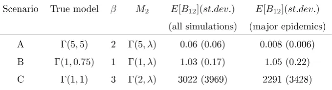
Table 3: Example 3: Bayes factors from MCMC output.
Scenario True model β M2 E[B12](st.dev.) E[B12](st.dev.)
(all simulations) (major epidemics)
A Γ(5,5) 2 Γ(5, λ) 0.06 (0.06) 0.008 (0.006)
B Γ(1,0.75) 1 Γ(1, λ) 1.03 (0.17) 1.05 (0.22)
C Γ(1,1) 3 Γ(2, λ) 3022 (3969) 2291 (3428)
to as major epidemics. The numbers of major epidemics were 63, 56 and 65 for
scenarios A, B and C, respectively.
Table 3 contains a summary of the Bayes factors estimated from the
sim-ulated data sets. In scenarios A, B and C the true models are M2, both M1
andM2, andM1respectively. The estimated Bayes factors behave as we might
expect, giving clear evidence in favour of modelsM2andM1for scenarios A and
C respectively, whilst for scenario B the mean ofB12 is close to the true value
of 1. In scenario A there is a marked difference in the Bayes factors when using
all simulations compared to using only major epidemics. A possible explanation
is that major epidemics contain more data, and so any difference between the
models becomes easier to detect. There is a less pronounced difference in Bayes
factors in scenario C, although the large posterior standard deviations suggest
there is no compelling evidence for a clear difference in this case.
4.4
SIR epidemic model vs. Poisson process
Our final example is motivated by the situation in which we wish to decide
whether observed cases of disease are the result of an epidemic (with
transmis-sion between individuals) or simply sporadic events. Specifically, suppose we
observe n events at times 0 < r1 < . . . < rn < T, and let r = (r1, . . . , rn).
Under modelM1,ris a vector of event times of a homogeneous Poisson process
of rateλobserved during the time interval [0, T]. Under modelM2, ris a
vec-tor of removal times in an SIR epidemic model with exponentially distributed
As for the previous example, we proceed by adding unobserved infection
times in order to obtain a tractable likelihood forM2. For simplicity we assume
that there is one initial infective at time zero, and furthermore that there is
a population of N individuals in total, where N ≥ n. Unlike the previous example, in which we unobserved infection times with observed removal times,
we here definei = (i2, . . . , im) to be a vector of m ordered infection times, so that 0 =i1 < i2< . . . , < im, wheren≤m≤N. The reason for this approach is that it appears to be easier when it comes to assigning missing data prior
densities, as described below. Note also that underM2we allow the possibility
that the epidemic is still in progress at timeT.
The likelihood for M1 and augmented likelihood for M2 are respectively
given by
π1(r|λ) = λnexp{−λT},
π2(i, r|β, γ) = ∏m
j=2
βS(ij−)I(ij−)
∏n
j=1
γI(rj−)
exp
{
−
∫ T
0
βS(t)I(t) +γI(t)dt
}
.
To proceed we require a missing data prior densityπ1(i|r, λ, β, γ). Now for a
given ordered vector of event timesr, π2(i, r|β, γ)>0 if and only if i∈ F(r),
where
F(r) ={i:i1< i2< . . . < im< T;ik< rk−1, k= 1, . . . , n+ 1;ik < T, k=n+ 2, . . . , m}. One way to defineπ1(i|r, λ, β, γ) is via the following construction, which
sim-ulates an element ofF(r). First, select maccording to some probability mass functionf on {n, n+ 1, . . . , N}. Next, sequentially set i2 ∼ T rExp(µ;i1, r1),
i3∼T rExp(µ;i2, r2), . . .,in+1∼T rExp(µ;in, rn),in+2∼T rExp(µ;in+1, T), . . .,
im∼T rExp(µ;im−1, T), whereT rExp(µ;a, b) denotes an exponential random
variable with rate µ, truncated to the interval (a, b). This in turn induces a
probability distribution with density
π1(i|r) =f(m)
m∏−1
j=1
µexp(−µij)
exp(−µij−1)−exp(−µsj−1)
, i∈ F(r),
where sj = rj for j = 1, . . . , n and sj = T for n < j ≤ m, and we set
We remark that it is not necessary to define the missing data prior density in
this manner. For instance, one could proceed by choosingmas before and then
assigning a uniform density to the set {i:i2< i3< . . . < im}. The practical drawback with this is that, if using allocation variables, the Markov chain can
never leave modelM1 ifiis such thatπ2(i, r|β, γ) = 0.
Prior distributions were assigned as β ∼ Γ(νβ, µβ), γ ∼ Γ(νγ, µγ), λ ∼ Γ(νλ, µλ) andα1∼Beta(p1, p2).
An MCMC algorithm is easily developed in a similar manner to the previous
example. Specifically we have the following full conditional distributions:
α1| · · · ∼ Beta(z1+p1,1−z1+p2),
z1| · · · ∼ Bern (
α1π1(r|λ)π1(i|r)
α1π1(r|λ)π1(i|r) + (1−α1)π2(i, r|β, γ) )
,
λ| · · · ∼
Γ(νλ, µλ) z1= 0,
Γ(n+νλ, T +µλ) z1= 1,
β| · · · ∼
Γ(m−1 +νβ,
∫T
0 S(t)I(t)dt+µβ) z1= 0,
Γ(νβ, µβ) z1= 1,
γ| · · · ∼
Γ(n+νγ,
∫T
0 I(t)dt+µγ) z1= 0,
Γ(νγ, µγ) z1= 1.
Updates for i are achieved as follows. If z1 = 1 then i has full conditional
densityπ1(i|r) which can be sampled as described above. Ifz1 = 0 theni can
be updated by moving, adding or deleting infection times as described in O’Neill
and Roberts (1999).
To illustrate this algorithm we considered a data set taken from an outbreak
of Gastroenteritis described in Britton and O’Neill (2002) which take the form
of 28 case detection times among a population of 89 individuals. The daily
numbers of cases on days 0 to 7 are given respectively by
1,0,4,2,3,3,10,5.
Strictly speaking, such data should be analysed by allowing the unknown time
Since our main objective here is to illustrate our methodology, we instead make
the simplifying assumption that day 0 actually corresponded to the start of the
outbreak, and then consider the remaining 27 case detection times.
For the missing data prior densityπ1(i|r) we set
f(m) = (1−θ) m−nθ
1−(1−θ)N−n+1, m=n, . . . , N,
so that m has a truncated Geometric distribution with parameter θ, and set
µ= 4 in the truncated exponential distribution.
We ran the algorithm with two choices ofT, the time of observation, withβ,
γandµall givenExp(1) prior distributions. First, withT = 10 we estimated the
Bayes factor in favour of the Poisson model to be 0.003, here usingp1= 400, p2=
1 to obtain reasonable mixing in the MCMC algorithm. So in this case there
appears to be overwhelming evidence to suggest that the case detection times are
better described by an epidemic model than a Poisson process. Second, we set
T = 3.5 and used only the case observation times up until day 3. We estimated
the Bayes factor in favour of the Poisson model to be 21.1. In comparison to
theT = 10 case we would certainly expect a value closer to 1, since there are
less data, and equally it is intuitively reasonable that there are insufficient data
to provide evidence in favour of an epidemic.
5
Discussion
We have presented a new method for evaluating Bayes factors. Although
mo-tivated by epidemic models and population processes, our approach is clearly
applicable in more general settings, as illustrated by the pines data set example
in Section 4.
The methods we propose are not without drawbacks. First, in common with
the product-space methods it seems likely that they are best suited to
situa-tions in which there are only a small number of competing models, although we
have not investigated this issue in this paper. Second, constructing missing data
in order to obtain reasonably efficient algorithms. Intuitively we expect that it
is best to choose missing data prior distributions to mimic the true distribution
of missing data in competing models. These aspects, as well as the method in
general, appear worthy of more detailed exploration.
AcknowledgementWe thank Christian Robert and Andy Wood for helpful
discussions about this work. We acknowledge funding from UK EPSRC grant
EP/F017006/1.
References
Andersson, H. and T. Britton (2000). Stochastic Epidemic Models and their Statistical Analysis. New York: Springer.
Britton, T. and P. D. O’Neill (2002). Bayesian inference for stochastic epidemics
in populations with random social structure. Scand. J. Statist. 29(3), 375– 390.
Brooks, S., P. Giudici, and G. Roberts (2003). Efficient construction of reversible
jump Markov chain Monte Carlo proposal distributions. J. R. Statist. Soc. B 65, 3–39.
Carlin, B. P. and S. Chib (1995). Bayesian model choice via Markov chain
Monte Carlo methods. J. R. Statist. Soc. B 57(3), 473–484.
Celeux, G., F. Forbes, C. Robert, and D. Titterington (2006). Deviance
Infor-mation Criteria for missing data models. Bayesian Analysis 1, 651–674.
Dellaportas, P., J. Forster, and I. Ntzoufras (2002). On Bayesian model and
variable selection using MCMC. Statistics and Computing 12(1), 27–36.
Dempster, A., N. Laird, and D. Rubin (1977). Maximum likelihood from
Diebolt, J. and C. P. Robert (1994). Estimation of finite mixture distributions
through Bayesian sampling. J. R. Statist. Soc. B 56(2), 363–375.
Friel, N. and A. N. Pettitt (2008). Marginal likelihood estimation via power
posteriors. J. R. Stat. Soc. Ser. B 70(3), 589–607.
Godsill, S. J. (2001). On the relationship between markov chain monte carlo
methods for model uncertainty. Journal of Computational and Graphical Statistics 10(2), 1–19.
Green, P. J. (1995). Reversible jump Markov chain Monte Carlo computation
and Bayesian model determination. Biometrika 82(4), 711–732.
Green, P. J. (2003). Transdimensional Markov chain Monte Carlo. In P. J.
Green, N. L. Hjort, and S. Richardson (Eds.), Highly Structured Stochastic Systems, pp. 179–98. Oxford: OUP.
Green, P. J. and A. O’Hagan (1998). Model choice with MCMC on product
spaces without using pseudo-priors. Technical Report, Department of Mathe-matics, University of Nottingham.
Han, C. and B. P. Carlin (2001). Markov Chain Monte Carlo Methods for
Computing Bayes Factors: A Comparative Review. Journal of the American Statistical Association 96(455), 1122–1132.
H¨ohle, M. and P. D. O’Neill (2005). Inference in disease transmission
experi-ments by using stochastic epidemic models. Appl. Statist. 54(2), 349–366.
O’Neill, P. D. and G. O. Roberts (1999). Bayesian inference for partially
ob-served stochastic epidemics. J. Roy. Statist. Soc. Ser. A 162, 121–129.
Richardson, S. and P. J. Green (1997). On Bayesian analysis of mixtures with
an unknown number of components. J. R. Statist. Soc. B 59(4), 731–792.
Streftaris, G. and G. J. Gibson (2004). Bayesian inference for stochastic
Williams, E. J. (1959). Regression analysis. A Wiley Publication in Applied Statistics. New York: John Wiley & Sons Inc.
6
Appendix
6.1
Proof of Lemma 1
(a) Define
b= [B1k(x)· · ·Bnk(x)]T,
so that (5) can be written as the matrix equation Ab=0. SinceBkk(x) = 1,
we can rewrite (5) as
∑
j̸=k
AijBjk(x) =−Aik, i= 1, . . . , n. (8) Now, for 1≤l, j≤n,
Alj = E[αl|x]E[αj]−E[αlαj] = E[αj]
1−∑
i̸=l
E[αi|x]
−E
1−∑
i̸=l
αi
αj
= −∑
i̸=l
(E[αj]E[αi|x]−E[αiαj])
= −∑
i̸=l
Aij. (9)
Summing (8) overi̸=kand using (9) now yields
∑
i̸=k
∑
j̸=k
AijBjk(x) = −
∑
i̸=k
Aik
so ∑
j̸=k
∑
i̸=k
Aij
Bjk(x) = −∑ i̸=k
Aik
so ∑
j̸=k
AkjBjk(x) = −Akk,
which is the equation obtained from (8) wheni =k. In other words, at least
system of equations defined by
˜
A−kb˜= ˜c, (10)
where ˜bis the (n−1)×1 column vector formed by removingBkk(x) = 1 from
b, and ˜cis the (n−1)×1 column vector with components−Aikfori= 1, . . . , n,
i̸=k. Application of Cramer’s rule to solve (10) now yields part (a).
(b) For the second part, we require some preliminary results. WriteE[αi|x] =
f(mi(x)), say. From (4) we have
f(mi(x)) =
∑n
j=1E[αiαj]mj(x)
∑n
j=1E[αj]mj(x)
=
∑
j̸=iE[αiαj]mj(x) +E[α2i]mi(x)
∑
j̸=iE[αj]mj(x) +E[αi]mi(x)
.
Differentiation yields thatf′(mi(x))≥0 if and only ifC≥0, where
C=∑ j̸=i
(E[α2i]E[αj]−E[αi]E[αiαj])mj(x). Thus ifC≥0 we obtain the bounds
∑
j̸=iE[αiαj]mj(x)
∑
j̸=iE[αj]mj(x) ≤
E[αi|x]≤
E[α2
i]
E[αi], (11)
and moreover the lower and upper bounds are attained when mi(x) = 0 and
mi(x) → ∞, respectively. In particular, for C >0 and 0 < mi(x)<∞ then both inequalities are strict. IfC ≤ 0 then the inequalities in (11) are simply reversed. From now on we assume that 0< mi(x)<∞for alli= 1, . . . , n.
Now ifn= 2 then (11) yields that fori̸=j,
E[α1α2]
E[αj]
̸
=E[αi|x],
from which it follows that Aij =E[αi|x]E[αj]−E[α1α2] ̸= 0. The result for
n= 2 now follows directly from part (a).
For the final part, in whichαhas a Dirichlet prior distribution, we first show
We start with conditions under whichC >0. Specifically, if Cov(αi, αj)<0
for alli̸=j and Var(αi)>0 then
E[αi]E[αj] > E[αiαj]
so E[αi2]E[αi]E[αj] > E[αi]2E[αiαj],
from which it follows thatC >0.
Next, suppose thatα∼ D(p1, . . . , pn) and setp0= ∑n
i=1pi. Thus fori̸=j,
E[αiαj] = pipj/(p0(p0 + 1)), E[αi] = pi/p0, E[α2i] = pi(pi + 1)/p0(p0 + 1),
Cov(αi, αj)<0 and Var(αi)>0. It follows thatC >0 and that (11) simplifies
to
pi
pi+ 1
< E[αi|x]<
pi+ 1
p0+ 1
. (12)
Next, note that fori̸=j we have
Aij = E[αj]E[αi|x]−E[αiαj] = pj
p0 (
E[αi|x]−
pi
p0+ 1 )
= bjai(x),
say, wherebj=pj/p0. It follows from (12) thatAij >0. Similarly
Aii =
pi
p0 (
E[αi|x]−
pi+ 1
p0+ 1 )
= bi˜ai(x),
say. Recall that ˜A−k is the matrixA with thekth row and column deleted. It
now follows that
det( ˜A−k) =
∏
i̸=k
bi
det(D+E),
where D is an (n−1)×(n−1) diagonal matrix with entries ˜ai(x)−ai(x) =
−1/(p0+ 1),i̸=k, andE is an (n−1)×(n−1) matrix consisting of (n−1)
Now from the matrix determinant lemma,
det(D+uvT) = (1 +vTD−1u)det(D),
and since det(D) = (−1/(p0+ 1))n−1̸= 0, we focus on 1 +vTD−1u. Now
1 +vTD−1u = 1−∑ i̸=k
(p0+ 1)ai(x)
= 1−∑
i̸=k
[(p0+ 1)E[αi|x]−pi]
= 1−(p0+ 1)(1−E[αk|x]) + (p0−pk) = E[αk|x](p0+ 1)−pk>0,
where the last inequality follows from (12). Hence det ˜A−k̸= 0 as required. Finally, we show that fori̸=k, (8) is satisfied by Bjk(x) =Ajk/Akj. First, it is straightforward to show that fori̸=k,
˜
ai(x) + ∑ j̸=k;j̸=i
aj(x) =−ak(x). (13) Now,
∑
j̸=k
Aij
Ajk
Akj
= bi˜ai(x)bkai(x)
biak(x)
+ ∑
j̸=k;j̸=i
bjai(x)
bkaj(x)
bjak(x)
= ai(x)bk
ak(x)
˜ai(x) + ∑ j̸=k;j̸=i
aj(x)
= ai(x)bk
ak(x) (−ak(x)) = −Aik,
using (13). Hence fori̸=k, (8) is satisfied byBjk(x) =Ajk/Akj as required.
Example 1To illustrate the calculations in part (a), consider the casen= 3,
k= 1. The equationAb=0is
A11 A12 A13
A21 A22 A23
and so
˜
A−1=
A22 A23
A32 A33 , b˜ =
B21
B31 , c=
−A21
−A31 .
Applying Lemma 1 yields
B21=
det ˜A−21
det ˜A−1
= det
−A21 A23
−A31 A33
det ˜A−1
, B31=
det ˜A−31
det ˜A−1
= det
A22 −A21
A32 −A31
det ˜A−1
.
Example 2To show thatBjk(x) does not equalAjk/Akjin general, suppose
thatn= 3, thatmi(x) =ifori= 1,2,3, and thatαhas a mixed Dirichlet prior
distribution given by
α∼(0.5)D(1,1,1) + (0.5)D(1,2,1).
Direct calculation then yields thatE[α1] =E[α3] = 7/24,E[α2] = 10/24 and
E[α2
1] E[α1α2] E[α1α3]
E[α2α1] E[α22] E[α2α3]
E[α3α1] E[α3α2] E[α23] = 1 20
2 2 1
2 6 2
1 2 2
,
whence E[α1|x] = 31/120, E[α2|x] = 50/120 and E[α3|x] = 39/120. Thus