Fault Classification and Localization in Power Systems
Using Fault Signatures and Principal Components Analysis
Qais H. Alsafasfeh1, Ikhlas Abdel-Qader2, Ahmad M. Harb3,4
1Electrical Engineering Department, Tafila Technical University, Tafila, Jordan
2Department of Electrical and Computer Engineering, Western Michigan University, Kalamazoo, USA 3Energy Engineering Department, German Jordanian University, Amman, Jordan
4School of Natural Resources Engineering, Jordan University of Science and Technology, Amman, Jordan Email: [email protected], [email protected]
Received May 4, 2012; revised June 20, 2012; accepted July 5,2012
ABSTRACT
A vital attribute of electrical power network is the continuity of service with a high level of reliability. This motivated many researchers to investigate power systems in an effort to improve reliability by focusing on fault detection, classi-fication and localization. In this paper, a new protective relaying framework to detect, classify and localize faults in an electrical power transmission system is presented. This work will extract phase current values during (1 4)th of a cycle to generate unique signatures. By utilizing principal component analysis (PCA) methods, this system will identify and classify any fault instantaneously. Also, by using the curve fitting polynomial technique with our index pattern obtained from the unique fault signature, the location of the fault can be determined with a significant accuracy.
Keywords: Fault Detection and Classification; Protective Relaying; PCA; PSCAD
1. Introduction
Fault detection and localization is a focal point in the research of power systems area since the establishment of electricity transmission and distribution systems. The objectives of a power system fault analysis is to provide enough information to understand the reasons that lead to an interruption and to, as soon as possible, restore the handover of power, and perhaps minimize future occur-rences if possible at all. Analysis should indeed provide us with an understanding of the network that can lead to producing a set of preventive measures which can be implemented to reduce the likelihood of equipment damage. Circuit breakers and other control elements are designed to help protective relays to take appropriate actions [1,2] and thus minimize damage and length of interruption. Prompt detection of a fault will have a sig-nificant impact on the equipment safety since it will en-gage the circuit breakers instantaneously and before any significant damage occurs. In recent years, with an in-crease in the number of power system networks within one control center, the behavior and effect of faults be-came more complex and as a result, fault impacted area has expanded. Researchers in applied mathematics and signal processing have developed many techniques for the detection, classification and localization of faults in electrical power systems and used them in conjunction with relaying and protection devices. Recent tools
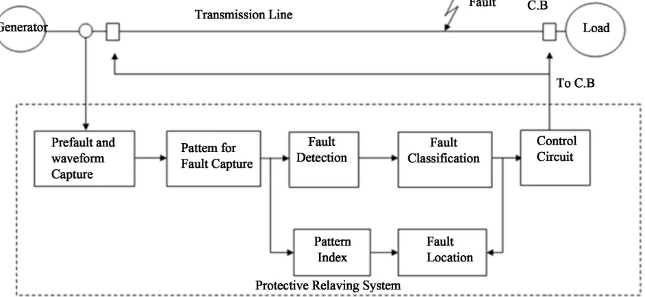
not investigated for real time implementation [4]. There is a need for new algorithms that have high efficiency, general applicability, and suitable for real time usage. In this work, we present a protection scheme consisting of three stages; the first stage includes the fault detection and classification based on patterns generated from phase current while the second stage is to initiate the classifica-tion process via PCA to declare the occurrence of a fault, if any, and its type. For the third stage, and once a fault is declared, a localization process is initiated to determine the fault location by combining our pattern indices gen-erated from the unique fault signatures and the polyno-mial curve fitting technique. This framework is illus-trated in Figure 1.
[image:2.595.382.497.190.265.2]2. Signature Estimation of Fault Signal
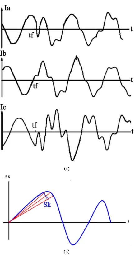
Figure 2 represents a 3-phase system signals in the time domain extracted from a power system. In Part a, the three current signals from each phase are shown while part b is showing the diagram of the difference signal, S, from an unbalanced three-phase system.The difference signal S between current signal and its previous reading at each (1 4)th of a cycle is gene- rated at the sending end of the transmission line. The difference signal, shown in Figure 2(b), at each instant of time is assumed to model a line equation of the form:
0
Bt C
A S (1) where A, B and C are constant derived from line specific intersect points. Once S is modeled using the line equa-tion given in Equaequa-tion (1), it is used to transform the data into a phasor domain by transforming each value of the difference signal as a magnitude and phase of its line
tors in the ρ-λ space as
0
B
C A
B
(2)
The magnitude and phase values for this new vector representation are computed using Equations (3) and (4) as follows:
2
2 C
r B A B
(3)
1 tan
C A
B B
(4) where r and k are the mathematical magnitude and
phase at each value of the S signal, respectively. Con-sidering three variables for the three phases a, b, and c, we will produce the following 3-phase set of equations:
1 1 1
1 1 1
1 1 1
ia ia
ib ib
ic ic
r r r r r r
(5)
where r1ia , r1ib , and 1ic are the mathematical
magnitude values at one instant of S signal for phase a,
b, and c, receptively and 1
r
, 1, and 1 are the mathematical phase values at one instant of the of S signal for phase a, b and c, receptively. Our data trans-formation is followed by a transtrans-formation into symme- trical components via the symmetrical components tech-nique [17], which allows for systematic analysis and
[image:2.595.65.536.492.709.2](a)
[image:3.595.65.282.78.488.2](b)
Figure 2. Unbalanced system signals: (a) each phase signal and (b) difference signal of current wave for phase a under a fault condition.
design of three phase systems as shown in Equation (6). In the left hand side of Equation (6) are the sought sym-metric quantities while the right hand side is the system phasor quantities. In Equation (7) we replace the phasor quantities of Equation (6) by our transformed data of the difference signal S,
0 2 1 1 1 1 3 1 a 2 1 a a b a c I I
I a a I
I a a I
(6) 1 1 1 2 0 1 1 1 3 1 1 ia ia ia P P a P 1 2 1 1 1 ia ib ic
a a r a r r (7)
This allows us to capture the symmetric components
of S by generating positive and negative patterns of each instant. Hence for total k samples, the symmetrical components will be:
1 1 1 21 1 1
2
1 1 1
0
1 1 1
2 2 0 1 3 1 , 3 1 3 1 3 1 , 3 1 3 ia ia ia k ia k ia k ia
a b c
a b c
a b c
k a k b k c
k a k b k c
k a k b k c
P r a r ar
P r ar a r
P r r r
P r a r ar
P r ar a r
P r r r
(8) Leading to 2 2 0 1 1 1 3
1 1 1
k a k
k ia
k ia k b k
k ia k c k
r
P a a
P a a r
P r P
By computing k ia and Pk ia
1 2 3
1 2 3
, , , ,
, , , ,
ia ia ia ia k ia
ia ia ia ia k ia
P P P P P P P P P P
over a time series all within (1/4)th of a cycle, we generate, shown in Equation (9), the positive and negative signatures which is a model for any unbalanced and nondeterministic time three- phase system which was allowed by symmetrical com-ponents method utilization.
(9)
[image:3.595.119.268.612.716.2]
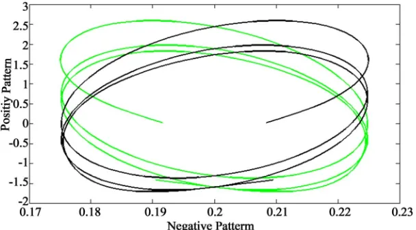
Figure 3 shows a plot of the unique signature of phase a in a 3-phase system with a fault a-g only while samples of other signatures are shown in the experimental work in Section 4.
The output of this process will then be supplied into the classification process to detect the fault and obtain a classification for the event. This proposed work is im-plemented and simulated using several PSCAD simula-tions. In Figure 4 a functional block diagram for the framework steps is shown.
3. Principal Component Analysis (PCA)
Based Fault Detection and Classification
Method
Figure 3. A plot of the unique signature of phase a in a 3-phase system with a fault a-g only.
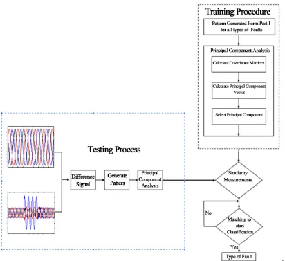
Figure 4. Detailed procedure followed to generate the sig-natures; difference signal is used thought data transforma-tion and symmetrical component method to obtain a unique signature of every event.
components (PCs) are calculated using the covariance ma- trix after a simple normalization procedure. The covari-ance matrix is, then calculated for these patterns simply as
cov ,
1
ia ia ia ia
ia ia
P P P P P P
k
P
(10) where ia and Pia, generated earlier per Equation (9),
are the positive and negative patterns respectively, Pia
and ia
the mean of
ia
P P, ia respectively, and k is the
number of samples used. Projection into the PC space is performed by using
P
i i i
C (11) where C is the covariance matrix; αi is the principal component in the ith dimension and
i
is its corre-sponding eigenvalue. Projecting the normalized data
PiaPia ,
PiaPia
onto the principal components, a new vector of data will be generated (PC1, PC2). Ac-company the usage of PCA for feature extraction is the usage of a similarity measure usually as a distance meas-ure. These may include Chebyshev, Euclidean, Manhat-tan, City Block, Canberra, and Minkowski, [22,23]. In this paper, the Euclidean distance measure is adapted as shown in Equation (12).
2 1 tested 1 stored
2 2 tested 2 stored
x i i
y i i
d PC PC
d PC PC
(12)minimum distance between the stored projections and test one. This minimum distance will identify a match of a pattern to a fault or no fault at all. In Figure 5 we dis-play the general framework for fault classification.
4. Experimental Results on Fault Detection
and Classification
Using the simulation package PSCAD, transmission line model shown in Figure 6 is used to simulate our frame-work. The network is composed of two sources, 220 kv each, that are connected by the transmission line with zero sequence parameter Z(0) = 82.5 + j308 Ω and a positive sequence impedance Z(1) = 8.25 + j94.5 Ω while ES = 220 kv and ER = 220∠δ kv.
We also, to show the validity of our algorithm on a more complex network, simulate our framework using a 6 bus network as shown in Figure 6(b). For this bus, the source voltages are at 400 kv each and the transmission line parameters are the same as the previous transmission
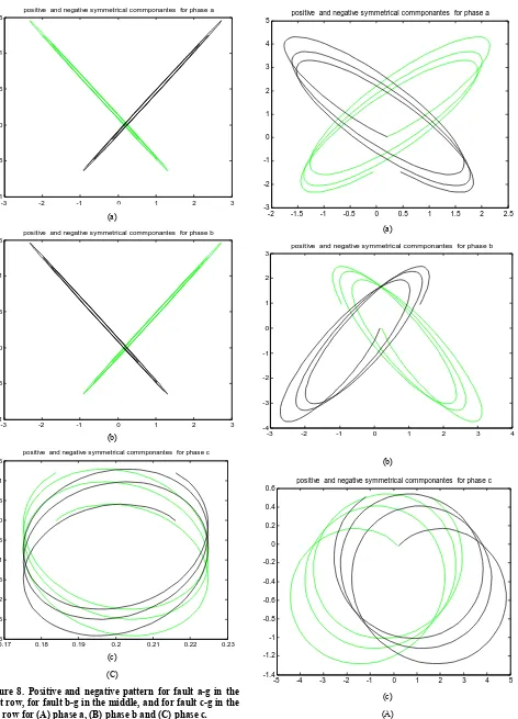
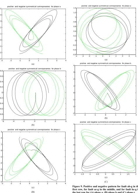
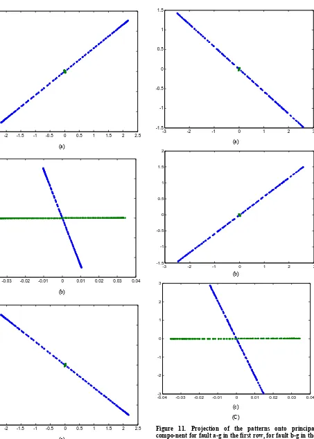
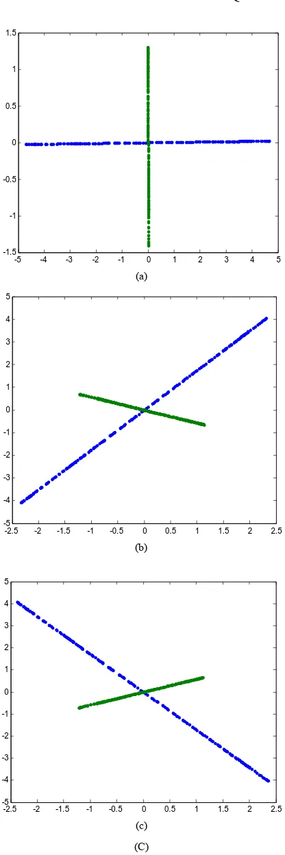
line model. Positive and negative patterns for the 3-phase system are displayed by Figures 7-10 and classification results are presented in Tables 1 and 2. The result of “No Fault” is the healthy condition event which we show its pattern in Figure 7. It is clear from Figure 7 that the sig-nature of each event is completely unique. A viewer for the signatures can easily identify the pattern of the faulty phase and declare the type of the fault from Figures 8 and 9. Projections into PCA results are also demonstrated in Figures 10-12. The Power system fault classifier was tested to classify the faults into a-g, b-g, cg, ab-g, ac-g, bc-g, ab, ac, bc, or abc using a total 220 samples for testing.
[image:5.595.93.505.329.706.2]Classification accuracy is presented in the confusion matrix in Table 1. These results were obtained with one template/pattern in the training data set. Table 2 displays the results storing two templates in the training set. The error percentage in the later case is zero. Results are con-sidered to be of significant improvement over the tradi-tional approaches.
positive and negative symmetrical commponantes for phase a 0.025
(a)
[image:6.595.57.290.81.376.2](b)
Figure 6. Using PSCAD simulation package, our framework was tested using (a) a 220 kv transmission lines and (b) a 400 kv 6-bus network.
5. Fault Localization
This framework can also be expanded to include a fault localization procedure. In this paper, the fault location is calculated by combining the curve fitting polynomial technique with our unique pattern indices that are gener-ated from the signatures as follows:
Index Index Index Index 2 2 2 2 index k a k a k a k a k va k ia k va k iak va k k va k
k ia k k ia k
k va k k va k
k ia k k ia k
P P P P P P
r a r P
r a r r a r P
r a r P Index Index 1 1 index k a k a k i k i P
k va k
k ia k
k va k
k ia k
a r a r a r a r
dex index
(13) where a, a are the positive and negative
Pattern indices for phase a. Using curve fitting, a training set is produced for the positive and negative pattern
in
0.17 0.18 0.19 0.2 0.21 0.22 0.23 -0.025 -0.02 -0.015 -0.01 -0.005 0 0.005 0.01 0.015 0.02 (a)
positive and negative symmetrical commponantes for phase b 0.025
0.17 0.18 0.19 0.2 0.21 0.22 0.23 -0.025 -0.02 -0.015 -0.01 -0.005 0 0.005 0.01 0.015 0.02 (b)
positive and negative symmetrical commponantes for phase c 0.025
[image:6.595.66.286.506.684.2]0.17 0.18 0.19 0.2 0.21 0.22 0.23 -0.025 -0.02 -0.015 -0.01 -0.005 0 0.005 0.01 0.015 0.02 (c)
Figure 7. Positive and negative pattern for each phase (phase a, phase b and phase c) for healthy condition.
0.17 0.18 0.19 0.2 0.21 0.22 0.23 -1.5
-1 -0.5 0 0.5 1 1.5 2 2.5 3 3.5
positive and negative symmetrical commponantes for phase a positive and negative symmetrical commponantes for phase a 1
(a)
-3 -2 -1 0 1 2 3
-2 -1.5 -1 -0.5 0 0.5 1
positive and negative symmetrical commponantes for phase b
(b)
-3 -2 -1 0 1 2 3
-2 -1.5 -1 -0.5 0 0.5 1
positive and negative symmetrical commponantes for phase c
(c) (A)
-1.5 -1 -0.5 0 0.5 1 1.5 2
-1 -0.8 -0.6 -0.4 -0.2 0 0.2 0.4 0.6 0.8
(a)
positive and negative symmetrical commponantes for phase b 2
0.17 0.18 0.19 0.2 0.21 0.22 0.23 -2
-1.5 -1 -0.5 0 0.5 1 1.5
(b)
positive and negative symmetrical commponantes for phase c 1
-1.5 -1 -0.5 0 0.5 1 1.5 2
-1 -0.8 -0.6 -0.4 -0.2 0 0.2 0.4 0.6 0.8
-3 -2 -1 0 1 2 3 -1
-0.5 0 0.5 1 1.5
positive and negative symmetrical commponantes for phase a positive and negative symmetrical commponantes for phase a 5
(a)
-3 -2 -1 0 1 2 3
-1 -0.5 0 0.5 1 1.5
positive and negative symmetrical commponantes for phase b
(b)
0.17 0.18 0.19 0.2 0.21 0.22 0.23 -3
-2.5 -2 -1.5 -1 -0.5 0 0.5 1 1.5
positive and negative symmetrical commponantes for phase c
[image:8.595.70.542.80.735.2](c) (C)
Figure 8. Positive and negative pattern for fault a-g in the first row, for fault b-g in the middle, and for fault c-g in the last row for (A) phase a, (B) phase b and (C) phase c.
-2 -1.5 -1 -0.5 0 0.5 1 1.5 2 2.5 -3
-2 -1 0 1 2 3 4
(a)
positive and negative symmetrical commponantes for phase b 3
-3 -2 -1 0 1 2 3 4
-4 -3 -2 -1 0 1 2
(b)
positive and negative symmetrical commponantes for phase c 0.6
-5 -4 -3 -2 -1 0 1 2 3 4 5
-1.4 -1.2 -1 -0.8 -0.6 -0.4 -0.2 0 0.2 0.4
positive and negative symmetrical commponantes for phase a
-3 -2 -1 0 1 2 3 4
-3 -2 -1 0 1 2 3 4 5
positive and negative symmetrical commponantes for phase a
1.4
(a)
-6 -4 -2 0 2 4 6
-1 -0.8 -0.6 -0.4 -0.2 0 0.2 0.4 0.6 0.8
positive and negative symmetrical commponantes for phase b
(b)
-3 -2 -1 0 1 2 3 4
-5 -4 -3 -2 -1 0 1 2 3
positive and negative symmetrical commponantes for phase c
(c) (B)
-4 -3 -2 -1 0 1 2 3 4 5
-0.6 -0.4 -0.2 0 0.2 0.4 0.6 0.8 1 1.2
(a)
positive and negative symmetrical commponantes for phase b 4
-3 -2 -1 0 1 2 3
-3 -2 -1 0 1 2 3
(b)
positive and negative symmetrical commponantes for phase c 3
-2 -1.5 -1 -0.5 0 0.5 1 1.5 2 -4
-3 -2 -1 0 1 2
[image:9.595.59.533.68.732.2](c) (C)
-0.04 -0.03 -0.02 -0.01 0 0.01 0.02 0.04
0.03 0.04 -0.04
-0.03 -0.02 -0.01 0 0.01 0.02
4
0.03
(a)
-0.04 -0.03 -0.02 -0.01 0 0.01 0.02 0.03 0.04 -0.04
-0.03 -0.02 -0.01 0 0.01 0.02 0.03 0.04
(b)
-0.04 -0.03 -0.02 -0.01 0 0.01 0.02 0.03 0.04 -0.04
-0.03 -0.02 -0.01 0 0.01 0.02 0.03 0.04
[image:10.595.100.535.80.726.2](c)
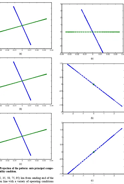
Figure 10. Projection of the patterns onto principal compo-nent for healthy condition.
tions (5, 25, 35, 50, 75, 95) km from sending end of the transmission line with a variety of operating conditions such as power angles and source impedance but at a spe-
-0.04-3 -0.03 -0.02 -0.01 0 0.01 0.02 0.03 0.04 -2
-1 0 1 2 3
(a)
1.5
-3 -2 -1 0 1 2 3
-2 -1.5 -1 -0.5 0 0.5 1
(b)
2
-3 -2 -1 0 1 2 3 -1.5
-1 -0.5 0 0.5 1 1.5
1.5
-2.5 -2 -1.5 -1 -0.5 0 0.5 1 1.5 2 2.5 -1.5
-1 -0.5 0 0.5 1 1.5
(a)
-0.04 -0.03 -0.02 -0.01 0 0.01 0.02 0.03 0.04 -3
-2 -1 0 1 2 3
(b)
-2.5 -2 -1.5 -1 -0.5 0 0.5 1 1.5 2 2.5 -1.5
-1 -0.5 0 0.5 1 1.5
(c) (B)
-3 -2 -1 0 1 2 3
-1.5 -1 -0.5 0 0.5 1
(a) 2
-3 -2 -1 0 1 2 3
-1.5 -1 -0.5 0 0.5 1 1.5
(b)
3
-0.04 -0.03 -0.02 -0.01 0 0.01 0.02 0.03 0.04 -3
-2 -1 0 1 2
[image:11.595.83.536.78.712.2](c) (C)
5
-2.5 -2 -1.5 -1 -0.5 0 0.5 1 4
1.5 2 2.5 -4
-3 -2 -1 0 1 2 3
(a)
-2.5 -2 -1.5 -1 -0.5 0 0.5 1 1.5 2 2.5 -4
-3 -2 -1 0 1 2 3 4
(b)
-5 -4 -3 -2 -1 0 1 2 3 4 5 -1.5
-1 -0.5 0 0.5 1 1.5
(c) (A)
-3 -2 -1 0 1 2 3 -5
-4 -3 -2 -1 0 1 2 3 4
(a) 1.5
-6 -4 -2 0 2 4 6 -1.5
-1 -0.5 0 0.5 1
(b)
5
-3 -2 -1 0 1 2 3 -5
-4 -3 -2 -1 0 1 2 3 4
-5 -4 -3 -2 -1 0 1 2 3 4 5 -1.5
-1 -0.5 0 0.5 1 1.5
(a)
-2.5 -2 -1.5 -1 -0.5 0 0.5 1 1.5 2 2.5 -5
-4 -3 -2 -1 0 1 2 3 4 5
(b)
-2.5 -2 -1.5 -1 -0.5 0 0.5 1 1.5 2 2.5 -5
-4 -3 -2 -1 0 1 2 3 4 5
[image:13.595.69.277.65.689.2](c) (C)
Figure 12. Projection of the patterns onto principal compo-nent for fault ab-g in the first row, for fault ac-g in the mid-dle, and for fault bc-g in the last row for (A) phase a, (B) phase B and (C) phase c.
cific fault resistance. To estimate the fault location, the positive and negative Pattern indices of the real inci-dent/test signals are determined and projected onto the fitted curve polynomial. An average of the two readings is taken as the fault location.
index
index
index
2
a a
a
D D
D
(14)
where D index
is the average distance of the previous estimates taken to be an accurate estimate of the fault location. The estimated distance in the first polynomial curve fitting is dependent on the specific value of the fault resistance and so if the fault to occur at a different values of fault resistance, that is, at a fault resistance not used in the first polynomial curve fitting, then an error in the distance estimate will occur. However, the error can be compensated by accounting for the difference in the fault resistance. That is, ∆R, the difference between the new fault resistance and the one used in the training, is used to generate a new polynomial curve to extract the corresponding ∆D. Upon testing and if there is any change in fault resistance then ∆D, the error in the dis-tance, will be added to the calculated fault distance as shown in (15).
index1
index2
index,
2
D D
D D D (15)
The error in fault location is given as (16).
Exact
Error D D 100%
L
D
(16) where D is the estimated fault distance, Exact is the
exact fault distance, and L is the transmission line total length, the functional block diagram as shown in Figure 13.
6. Experimental Results on Fault
Localization
Using the simulation package PSCAD, transmission line model shown in Figure 6(a) is used to simulate our framework. The network is composed of two sources, 220 kv each, that are connected by the transmission line with zero sequence parameter Z(0) = 82.5 + j308 Ω and a positive sequence impedance Z(1) = 8.25 + j94.5 Ω while ES = 220 kv and ER = 220∠δ kv.
Table 1. Classification performance using one template for each fault type in the training set producing a 94.54% average accuracy.
Confusion matrix Type of
fault Samples
a-g b-g c-g ab-g ac-g bc-g ab ac bc abc No fault Accuracy
a-g 20 20 0 0 0 0 0 0 0 0 0 0 100%
b-g 20 0 20 0 0 0 0 0 0 0 0 0 100%
c-g 20 0 0 20 0 0 0 0 0 0 0 0 100%
ab-g 20 0 0 0 20 0 0 0 0 0 0 0 100%
ac-g 20 0 0 0 0 20 0 0 0 0 0 0 100%
bc-g 20 0 0 0 0 0 20 0 0 0 0 0 100%
ab 20 0 0 0 0 0 0 20 0 0 0 0 100%
ac 20 0 0 0 0 0 0 0 20 0 0 0 100%
bc 20 0 0 0 0 0 0 0 0 20 0 0 100%
abc 20 0 0 0 0 0 0 0 0 0 20 0 100%
No fault 20 0 0 0 0 0 0 0 0 0 0 20 100%
Table 2. Classification performance by using two templates for each fault type in the training set producing 100% accuracy.
Confusion matrix Type of
fault Samples
a-g b-g c-g ab-g ac-g bc-g ab ac bc abc No fault Accuracy
a-g 20 19 0 0 0 0 0 0 0 0 0 1 95%
b-g 20 0 19 0 0 0 0 0 0 0 0 1 95%
c-g 20 0 0 20 0 0 0 0 0 0 0 0 100%
ab-g 20 0 0 0 18 0 0 2 0 0 0 0 90%
ac-g 20 0 0 0 0 20 0 0 0 0 0 0 100%
bc-g 20 0 0 0 0 0 18 0 0 2 0 0 90%
ab 20 3 0 0 0 0 0 17 0 0 0 0 85%
ac 20 0 0 0 0 0 0 0 20 0 0 0 100%
bc 20 0 0 0 0 0 0 0 0 17 0 3 85%
abc 20 0 0 0 0 0 0 0 0 0 20 0 100%
[image:14.595.56.538.438.726.2]Fault Type
Fault Location
Estimation Fault
Difference Signal (ΔV)
Difference Signal (ΔI)
Symmetrical Pattern
+ve,-veInd ex
Training Set between Symmetrical Pattern Index
and Fault location
Training Set for Fault Resistance
Error
Fault Type
Fault Location
Estimation Fault Resistance Difference Signal
(ΔV)
Difference Signal (ΔI)
Symmetrical Pattern Generation
+ve,-veInd ex
Training Set between Symmetrical Pattern Index and
Fault location
Tr Fa
aining Set for ult Resistance
[image:15.595.108.482.83.402.2]Error
Figure 13. Functional block diagram for fault location based on patterns indices.
Table 3. Fault location for different fault.
Fault location
Type of fault
Fault resistance
Estimated fault location km
Error
10 a-g 39 9.45 0.004
25 a-g 44 26.05 0.009
33 a-g 53 31 0.018
56 a-g 22 58.3 0.020
73 a-g 45 71.5 0.013
89 a-g 66 89.5 0.004
99 a-g 71 96 0.027
70 ab-g 35 69.08 0.009
15 ab-g 77 18 0.027
45 ab-g 40 44.6 0.003 80 ab-g 61 81.2 0.010 65 ab-g 57 67.4 0.021 54 ab-g 45 56.26 0.020
90 Ab 10 90.8 0.007
85 Ab 35 86.4 0.012
90 Ab 25 92.8 0.025
50 Ab 50 51.91 0.017
15 Ab 60 17 0.018
65 Ab 40 64.5 0.004
ditions. Maximum error is 2.7% in ab-g fault at 15 km from relaying point with fault resistance of 77 Ω and minimum error of 0.3% in ab-g at a 45 km from relaying point with fault resistance of 40 Ω. Table 4 shows the results for fault detection, classification and fault location for a 6 bus network with maximum error of 3% in cases of bc-g and ab faults with a 5 Ω and a 100 Ω fault resis-tance respectively. A functional block diagram for fault location based on patterns indices is shown in Figure 2.
7. Conclusions
[image:15.595.58.285.447.732.2]Table 4. Fault detection, classification and localization for a 6-bus network.
Fault type Fault section between bus Fault location Fault resistance angle Power δ Type of fault using algorithm fault locationEstimation Error
a-g 2-3 30 km from Bus 1 5 45° a-g 31 0.010
a-g 2-3 30 km from Bus 1 100 60° a-g 31.8 0.018
b-g 1-2 45 km from Bus 2 5 45° b-g 45.5 0.005
b-g 1-2 45 km from Bus 2 100 60° b-g 43 0.020
c-g 4-5 80 km from Bus 4 5 45° c-g 77.9 0.021
c-g 4-5 80 km from Bus 4 100 60° c-g 78 0.020
ab-g 2-3 30 km from Bus 1 5 45° ab-g 30.2 0.002
ab-g 2-3 30 km from Bus 1 100 60° ab-g 32.4 0.024
ac-g 1-2 45 km from Bus 2 5 45° ac-g 45.7 0.007
ac-g 1-2 45 km from Bus 2 100 60° ac-g 45.8 0.008
bc-g 4-5 80 km from Bus 4 5 45° bc-g 77 0.030
bc-g 4-5 80 km from Bus 4 100 60° bc-g 83 0.030
ab 2-3 30 km from Bus 1 5 45° ab 33 0.030
ab 2-3 30 km from Bus 1 100 60° ab 31 0.010
ac 1-2 45 km from Bus 2 5 45° ac 44 0.010
ac 1-2 45 km from Bus 2 100 60° ac 46.1 0.011
bc 4-5 80 km from Bus 4 5 45° bc 80.5 0.005
bc 4-5 80 km from Bus 4 100 60° bc 81.3 0.013
abc 2-3 30 km from Bus 1 5 45° abc 30.2 0.002
abc 2-3 30 km from Bus 1 100 60° abc 30.1 0.001
into a-g, b-g, cg, ab-g, ac-g, bc-g, ab, ac, bc, and abc with a total of 220 fault samples for algorithm simulation and testing. The classification accuracy was calculated to be at 94.54% using only one template per fault signature in the training set, and was improved to 100% by increasing the templates per fault signature to two. Determining fault location was also considered by combining poly-nomial curve fitting technique with the pattern index ratio of both the voltage signal and current signal unique signatures. The error in fault location is found to be be-low 2.7%. This proposed work is computationally simple, efficient, and can be used in real-time applications. This work can be easily expanded to more complex networks and can be used in distribution systems.
REFERENCES
[1] M. Kezunovic, et al., “Automated Fault Analysis Using Neural Network,” 9th Annual Conference for Fault and Disturbance Analysis, Texas A&M University, College Station, Texas, March 1994.
[2] M. Kezunovic and I. Rikalo, “Detect and Classify Faults
Using Neural Nets,” IEEE Computer Applications in Power, Vol. 9, No. 4, 1996, pp. 42-47.
doi:10.1109/67.539846
[3] K. Ferreira, “Fault Location for Power Transmission Systems Using Magnetic Field Sensing Coils,” Master Thesis, Worcester Polytechnic Institute, Worcester, April 2007.
[4] A. Jain, A. Thoke and R. Patel, “Fault Classification of Double Circuit Transmission Line Using Artificial Neural Network,” International Journal of Electrical and Elec-tronics Engineering, Vol. 1, No. 4, 2008, pp. 230-235. [5] A. Jain and A. Thoke, “Classification of Single Line to
Ground Faults on Double Circuit Transmission Line Us-ing ANN,” International Journal of Computer and Elec-trical Engineering, Vol. 1, No. 2, 2009, pp. 196-203. [6] M. Sanaye-Pasand and H. Khorashadi-Zadeh, “Transmis-
sion Line Fault Detection & Phase Selection Using ANN,” International Conference on PowerSystems Transients— IPST, New Orleans, 2003, pp. 1-6.
Conference on Power System Technology, Chongqing, 22-26 October 2006, pp. 1-5.
[8] K. S. Swarup, N. Kamaraj and R. Rajeswari, “Fault Di-agnosis of Parallel Transmission Lines Using Wavelet Based ANFIS,” International Journal of Electrical and Power Engineering, Vol. 1, No. 4, 2007, pp. 410-415. [9] V. Malathi and N. Marimuthu, “Multi-Class Support
Vector Machine Approach for Fault Classification in Power Transmission Line,” IEEE International Confer-ence on Sustainable Energy Technologies ICSET 2008, Singapore, 24-27 November 2008, pp. 67-71.
[10] S. El Safty and A. El-Zonkoly, “Applying Wavelet En-tropy Principle in Fault Classification, International,” Journal of Electrical Power & Energy Systems, Vol. 31, No. 10, 2009, pp. 604-607.
doi:10.1016/j.ijepes.2009.06.003
[11] J. Upendar, C. P. Gupta and G. K. Singh, “Discrete Wavelet Transform and Genetic Algorithm Based Fault Classification of Transmission Systems, National Power Systems Conference (NPSC-2008),” Indian Institute of Technology, Bombay, December 2008, pp. 223-228. [12] D. Biswarup and V. Reddy, “Fuzzy-Logic-Based Fault
Classification Scheme for Digital Distance Protection,” IEEE Transactions on Power Delivery, Vol. 20, No. 1, 2005, pp. 609-616.
[13] K. Razi, M. Hagh and G. Ahrabian, “High Accurate Fault Classification of Power Transmission Lines Using Fuzzy Logic,” International Power Engineering Conference IPEC, Singapore, 3-6 December 2007, pp. 42-46.
[14] S. Vaslilc and M. kezunovic, “Fuzzy ART Neural Net- work Algorithm for Classifying the Power System Faults,” IEEE Transactions on Power Delivery, Vol. 20, No. 2, 2005, pp. 1306-1314.
doi:10.1109/TPWRD.2004.834676
[15] S. Samantaray, P. Dash and G. Panda, “Transmission Line Fault Detection Using Time-Frequency Analysis,” IEEE Indicon 2005 Conference, Chennai, 2005, pp. 162-166.
[16] E. Styvaktakis, M. Bollen and I. Gu, “Automatic Classi-fication of Power System Events Using rms Voltage Measurements,” IEEE Power Engineering Society Sum-mer Meeting, Chicago, 25 July 2002, pp. 824-829. [17] H. Saadat, “Power System Analysis,” McGraw Hill, New
Yoek, 2002.
[18] I. Jollife, “Principal Component Analysis,” Verlag, Sprin- ger, 1986.
[19] J. Karhunen and J. Joutsensalo, “Generalizations of Prin- cipal Component Analysis, Optimization Problems, and Neural Networks,” Neural Networks, Vol. 8, No. 4, 1995, pp. 549-562. doi:10.1016/0893-6080(94)00098-7
[20] S. Nayar and T. Poggio, “Early Visual Learning,” Oxford University Press, New York, 1996.
[21] I. Abdel-Qader, S. Pashaie-Rad, O. Abudayyeh and S. Yehia, “PCA-Based Algorithm for Unsupervised Bridge Crack Detection,” Advances in Engineering Software, Vol. 37, No. 12, 2006, pp. 771-778.
doi:10.1016/j.advengsoft.2006.06.002
[22] D. Widdows, “Geometry and Meaning,” University of Chicago Press, Chicago, 2003.