c
° Indian National Science Academy DOI: 10.1007/s13226-019-0336-5
DYNAMICAL ANALYSIS OF A COMPLEX LOGISTIC-TYPE MAP
A. M. A. El-Sayed∗and S. M. Salman∗∗
∗Faculty of Science, Alexandria University, Alexandria, Egypt ∗∗Faculty of Education, Alexandria University, Alexandria, Egypt
e-mails: [email protected]; [email protected]
(Received 27 April 2018; after final revision 2 June 2018; accepted 4 July 2018)
A complex logistic-type map is considered in the present work. The dynamic behavior of the underlined map is discussed in two different cases: the first case is when the parameter of the map being real, and the second case is when the parameter being complex. Existence and stability of fixed points are derived. The conditions for existence of a pitchfork bifurcation, flip bifurcation and Neimark-Sacker bifurcation are derived by using the center manifold theorem and bifurcation theory. Numerical simulations including Lyapunov exponent, phase plane, bifurcation diagrams is carried out using matlab to ensure theoretical results and to reveal more complex dynamics of the map. The results show that expressing the logistic map in terms of complex variables leads to more distinguished behaviors, which could not be achieved in the logistic map with real variables. In addition, considering the control parameter as a complex parameter shows more interesting dynamics if compared to the case when considering it as a real parameter. Existence of a snapback repeller is proved in the sense of Marotto. Finally, chaos is controlled using the OGY feedback method.
Key words :Logistic-type map; complex variables; fixed points; local stability; Lyapunov expo-nent; bifurcation; chaos; OGY feedback control.
1. INTRODUCTION
In the last years, studies of the effect of forcing on systems simulated by the logistic mapxn+1 =
ρxn(1−xn) for choosing x0 between 0 and1 and0 < ρ < 4 have found a celebrated place in
relevant parameter sets for which this system behaves similarly concerning one or several properties of interest, such as, for example, periodicity of attractors and basins of attraction. Hyperchaos is known as a chaotic attractor with more than one positive Lyapunov exponent and actually has more rich dynamical behaviors than the usual chaos. Over the past decades, hyperchaotic systems with real variables have been investigated. Since Fowler et al. [5] introduced a complex Lorenz model which generalizes the real Lorenz model in 1982, chaotic and hyperchaotic complex systems have attracted attention to the systems with complex variables which can be used to describe the physics of a detuned laser, rotating fluids, disk dynamos, electronic circuits, and particle beam dynamics in high energy accelerators. In [6], the dynamics of hyperchaotic complex Chen system are investigated. When applying the complex systems in communications, the complex variables will double the number of variables and can increase the content and security of the transmitted information.
Periodic solutions are important in the study of dynamical systems, since they represent station-ary or repeatable behavior [7-9]. Non-linear differential equations with periodic coefficients are quite important from a periodical point of view. Especially, the search for periodic solutions of these equa-tions is an essential problem. Many problems of physical interest are concerned with the motion of strongly non-linear oscillators, see for example [10]. The main thrust of the present paper is to study the main dynamic behavior of the logistic map with complex variables. Actually, considering the logistic difference equation with complex variables is because complex analysis in one variable represents a portion of mathematical beauty, the real beauty and excitement comes in higher dimen-sions and manifolds (Riemann surfaces, complex manifolds, several complex variables) [11]. There are many examples of considering systems with complex variables, for example, the complex Lorenz equations, complex Chen and L¨u chaotic systems, complex logistic map, and complex Riccati map [12-16]. Indeed, the qualitative study of difference equations is a fertile research area and increasingly attracts many mathematicians. As a matter of fact, many real life phenomena are modeled using dif-ference equations. Examples from economy, biology, etc. can be found in [17-23]. Many non-linear systems have parameters which appear in the defining systems of equations. Changes may occur in the qualitative structure of the orbits for certain parameter values as the parameter varies [24]. The main problem in non-linear dynamics is that of determining how the properties of orbits may change and evolve as a parameter of a dynamical system is changed [25].
In this paper, we consider the logistic-type difference equation given in the form
zn+1=ρzn(1−znz¯n), n= 1,2,3, ... (1.1) whereρ∈R, with initial condition
wherez=x+iy,z¯=x−iy,|zn| ≤1andi=
√
−1. We are going to study the nonlinear dynamics of Eq. (1.1) such as stability of fixed points, local bifurcations analysis using bifurcation theory and center manifold theorem [26, 27], Lyapunov exponent, and chaos.
This paper is organized as follows, in Section 2 the existence and stability of the fixed points of the map (1.1) is presented when ρ is real. Qualitative behavior and local bifurcation analysis are discussed using center manifold theorem and bifurcation theory. Moreover, conditions for the existence of pitchfork bifurcation and flip bifurcation are derived. Section 3 represents qualitative behavior of map (1.1) in caseρ is complex. In addition, conditions for the existence of Neimark-Sacker (NS) bifurcation are given. Numerical simulations results are presented in Section 4 to verify our theoretical analysis and visualize the newly observed complex dynamics of the system. Finally, in Section 5 conclusion is given.
2. EXISTENCE ANDLOCALSTABILITY OFFIXEDPOINTSWHENρIS REAL
Rewrite Eq. (1.1) as
xn+1 =ρ(xn−x3n−xnyn2), n= 1,2,3, ...
yn+1 =ρ(yn−ynx2n−y3n). (2.1)
To find fixed points of system (2.1) we solve the following system of algebraic equations x = ρ(x−x3−xy2),
y = ρ(y−yx2−y3).
So, fixed points of system (2.1) are as follows:
•For all values ofρ, there is one fixed point only which is the originf ix1(0,0).
•Forρ >1, there are infinite number of fixed points since they lie inside the circle
½
Z∈C:|Z|2 = ρ−1 ρ
¾
.
For convenience, we will consider only here the obvious fixed points which are:f ix2
³
0,
q
ρ−1 ρ
´
, f ix3
³
0,−
q
ρ−1 ρ
´
,f ix4
³q
ρ−1 ρ ,0
´
, andf ix5
³
−
q
ρ−1 ρ ,0
´
. Note thatf ix2andf ix3are
symmet-ric aboutx−axis, whilef ix4 andf ix5are symmetric abouty−axis.
point(x∗, y∗)reads
J(x∗, y∗) =
Ã
ρ(1−3x∗2−y∗2) −2ρx∗y∗ −2ρx∗y∗ ρ(1−3y∗2−x∗2)
!
. (2.2)
In order to discuss the stability of the fixed point(x∗, y∗), we need the following lemma.
Lemma 1 — Let F(λ) = λ2+P λ+Q. Suppose thatF(1) > 0, λ1 andλ2 are two roots of
F(λ) = 0. Then
1. |λ1|<1and|λ2|<1if and only ifF(−1)<0,Q <1,
2. |λ1|<1and|λ2|>1(or|λ1|>1and|λ2|<1) if and only ifF(−1)<0,
3. |λ1|>1and|λ2|>1if and only ifF(1)>0andQ >1,
4. λ1 =−1and|λ2| 6= 1if and only ifF(−1) = 0andP 6= 0,2,
5. λ1andλ2 are complex and|λ1|= 1and|λ2|= 1if and only ifP2−4Q <0andQ= 1.
Letλ1 andλ2 be the two roots of the characteristic equation of the Jacobian matrixJ(x∗, y∗)
at the fixed point(x∗, y∗)which are called eigenvalues of the fixed point (x∗, y∗). We recall some definitions of topological types for a fixed point(x∗, y∗). A fixed point(x∗, y∗) is called a sink if |λ1|<1and|λ2|<1, so the sink is locally asymptotically stable; it is called a source if|λ1|>1and
|λ2|>1, so the source is locally unstable; it is called a saddle if|λ1|>1and|λ2|<1(or|λ1|<1
and|λ2|>1); and(x, y)is called non-hyperbolic if either|λ1|= 1or|λ2|= 1.
According to Lemma 1 and (2.2), we have the following propositions. Proposition 1 —f ix1(0,0)is:
A sink if−1< ρ <1, A source ifρ >1orρ <−1,
A non-hyperbolic ifρ= 1orρ=−1. Note thatf ix1can not be a saddle.
Proposition 2 —f ix2
³
0,
q
ρ−1 ρ
´
is a non-hyperbolic ifρ= 1orρ= 2. The same proposition can be applied tof ix4
³q
ρ−1 ρ ,0
´
. Note that bothf ix2andf ix4 can not
2.1 Bifurcation off ix1(0,0)
The Jacobian matrix atf ix1(0,0)reads
J(f ix1) =
Ã
ρ 0
0 ρ
!
, (2.3)
which has two eigenvaluesλ1,2 =ρ. Ifρ= 1, thenλ1,2= 1.
Lemma 2 — Ifρ= 1, system (2.1) undergoes a pitchfork bifurcation atf ix1(0,0). Moreover, the
system has only one fixed point.
PROOF: In the analysis of bifurcations we always takeρas a bifurcation parameter. Letµ=ρ−1 such that parameter µ be a new and dependent variable, the system (2.1) is transformed into the following form x y µ →
1 0 0 0 1 0 0 0 1
x y µ +
µ(x−x3−xy2)−x3−xy2
−yx2−y3+µ(y−yx2−y3)
0
. (2.4)
Then, there exists a center manifold for (2.4), which can be represented as follows: Wc(f ix1) ={(x, y, µ)∈R3|y=h(x, µ), h(0,0) =Dh(0,0),|x|< ²,|µ|< δ},
for²,δsufficiently small.
To compute the center manifoldWcwe assume
h(x, µ) =c0x2+c1xµ+c2µ2+O((|x|+|µ|)3), (2.5)
whereO((|x|+|µ|)3)is the sum of all terms whose order is great than 2. The center manifold must satisfy
h(x+µ(x−x3)−µxh(x, µ)2−x3−xh(x, µ)2, µ) =h(x, µ)−x2h(x, µ)−h(x, µ)3. (2.6)
Substituting (2.4) and (2.5) into (2.6) and then equating coefficients of like powers in (2.6), we get
c0= 0, c1 = 0, c2= 0
Thus the map restricted to the center manifold is given by
Since
³∂2F 1
∂x∂µ
´
(0,0) = 16= 0,
³∂3F 1
∂x3
´
(0,0) = −66= 0.
Thus, system (2.1) undergoes a pitchfork bifurcation atf ix1(0,0). This completes the proof. 2
Lemma 3 — Ifρ = −1, system (2.1) undergoes a flip bifurcation atf ix1(0,0). Moreover, the
stable periodic-2 point bifurcates from this fixed point.
PROOF: Ifρ=−1, the two eigenvalues of (2.3) becomeλ1,2 =−1.
Letµ=ρ+ 1be new and dependent variable, the system (2.1) is transformed into the following form x y µ →
−1 0 0
0 −1 0
0 0 −1
x y µ +
µ(x−x3−xy2) +x3+xy2
yx2+y3+µ(y−yx2−y3) 0
. (2.7)
Then, there exists a center manifold for (2.7), which can be represented as follows: Wc(f ix1) ={(x, y, µ)∈R3|y =h(x, µ), h(0,0) =Dh(0,0),|x|< ²,|µ|< δ},
for²,δsufficiently small.
To compute the center manifoldWcwe assume
h(x, µ) =a0x2+a1xµ+a2µ2+O((|x|+|µ|)3), (2.8)
whereO((|x|+|µ|)3)is the sum of all terms whose order is great than 2. The center manifold must satisfy
h(−x+µ(x−x3) +µxh(x, µ)2+x3+xh(x, µ)2, µ)
= (1−µ)h(x, µ)−µx2h(x, µ) +h(x, µ)3. (2.9) Substituting (2.7) and (2.8) into (2.9) and then equating coefficients of like powers in (2.9), we get
a0= 0, a1 = 0, a2 = 0
Thus the map restricted to the center manifold is given by
Since
α1 =
³
2∂2F2 ∂µ∂x +
∂F2 ∂µ
∂2F 2
∂x2
´
(0,0) = 26= 0,
α2 =
³1
2
³∂2F 2
∂x2
´2
+1 3
³∂3F 2
∂x3
´´
(0,0) = 26= 0,
Thus, system (2.1) undergoes a flip bifurcation atf ix1(0,0). This completes the proof. 2
2.2 Bifurcation off ix2
³
0,
q
ρ−1 ρ
´
In this part, we will investigate the local bifurcation analysis of the second fixed point of the system (2.1) using the center manifold theorem exactly as we did for the first fixed point. The Jacobian matrix of system (2.1) evaluated atf ix2reads
J(f ix1) =
Ã
1 0
0 −2ρ+ 3
!
, (2.10)
which has two eigenvaluesλ1 = 1, and λ2 = −2ρ+ 3. Ifρ 6= 1,2, then|λ2| 6= 1, however, the
conditions of the occurrence of pitchfork bifurcation atf ix2 are not satisfied. On the other hand, if
ρ= 1, we will have thatλ1,2 = 1. In the following lemma, we show that the conditions of occurrence
of pitchfork bifurcation atf ix2are satisfied whenρ= 1.
Lemma 4 — Ifρ = 1, system (2.1) undergoes a pitchfork bifurcation atf ix2
³
0,
q
ρ−1 ρ
´
. More-over, the system has only one fixed point.
PROOF: First of all we need to translatef ix2to the origin using the translation
ξn=xn, ηn=yn−
r
ρ−1 ρ .
Introduceµ=ρ−1as new and dependent variable, system (2.1) becomes
ξ η µ →
1 0 0 0 1 0 0 0 1
ξ η µ +
f(ξ, η, µ) g(ξ, η, µ)
0
, (2.11)
wheref(ξ, η, µ) =−(µ+ 1)
³
ξ3+ξη2+q µ µ+1ξη
´
, g(ξ, η, µ) =−(µ+ 1)
³
3qµµ+1η2+η3+ξ2η+q µ µ+1ξ2
´
−2µη.
Then, there exists a center manifold for (2.11), which can be represented as follows:
for²,δsufficiently small.
To compute the center manifoldWcwe assume
h(ξ, µ) =d0ξ2+d1ξµ+d2µ2+O((|ξ|+|µ|)3), (2.12)
whereO((|x|+|µ|)3)is the sum of all terms whose order is great than 2.
The center manifold must satisfy
h(ξ−(µ+ 1)(ξ3+ξh(ξ, µ)2+
r
µ
µ+ 1ξh(ξ, µ)), µ)
=h(ξ, µ)−(µ+ 1)
r
µ µ+ 1ξ
2−
−3(µ+ 1)
r
µ
µ+ 1h(ξ, µ)
2+
+h(ξ, µ)3+ (ξ2−2µ)h(ξ, µ).
(2.13)
Note that in order to equate coefficients in both sides, we should use binomial theorem for the term
q
µ
µ+1 as follows:
r
µ µ+ 1 =
µ
1 + 1 µ
¶−1 2
= 1− 1 2µ+
3 8µ2 +...
.
Substituting (2.11) and (2.12) into (2.13) and then equating coefficients of like powers in (2.13), we get
d0 = 0, d1(d21−1) = 0, d2= 0.
Ford1, we have eitherd1 = 0ord1 = ±1. After careful calculations, we found that pitchfork
bifurcation conditions are not satisfied whend1 = ±1. while when d1 = 0, pitchfork bifurcation
conditions are satisfied. Thus the map restricted to the center manifold is given by
F3 :ξn+1=ξn−(µ+ 1)
µ
ξ3n+ξn+
r
µ µ+ 1ξn
−O((|xn|+|µn|)6).
Now we have
³∂2F 3
∂x∂µ
´
(0,0) = −66= 0,
³∂3F 3
∂x3
´
(0,0) =
Thus, system (2.1) undergoes a pitchfork bifurcation atf ix2
³
0,
q
1−1ρ
´
. This completes the
proof. 2
We will not discuss the bifurcations of the fixed pointf ix3 because it has symmetrical structure
with f ix2. So, the process will be omitted here. The same thing can be said tof ix5 which has
symmetrical structure withf ix4.
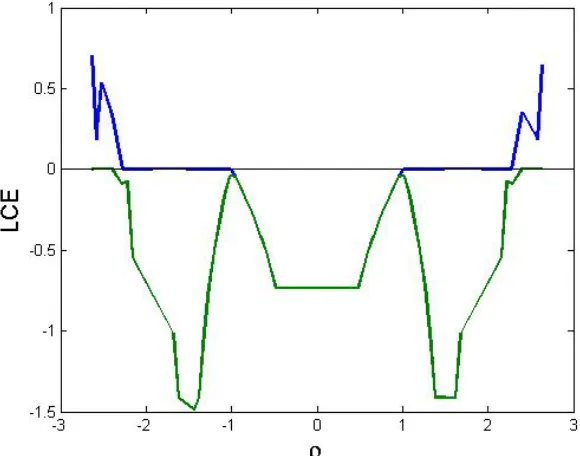
If one is interested in determining whether a dynamical system is chaotic or not, often just a few of the largest Lyapunov characteristic exponents (LCEs) may provide the answer. This actually because a positive LCE is a good indicator for chaos. Since for non-chaotic systems all LCEs are non-positive, the presence of a positive LCE has often been used to help determine if a system is chaotic or not. In this paper, we compute the (LCEs) via the Householder QR-based methods described in [28]. Figure 1 shows the LCEs for system (2.1) with the initial conditions (xo, yo) = (0.1,0.1). We find that
LCE1 =0.6443and LCE2 =0.0031.
3. EXISTENCE ANDLOCALSTABILITY OF FIXEDPOINTSWHENρISCOMPLEX
In this part, we considerρ=a+ib, wherea, b∈R. Eq. (1.1) is rewritten as xn+1=a(xn−x3n−xnyn2) +b(−yn+ynx2n+yn3),
[image:9.612.146.436.363.591.2]where n = 1,2,3, ..., |xn| ≤ 1, |yn| ≤ 1. Fixed points of system (3.1) are the solutions of the
following system of algebraic equations
x = a(x−x3−xy2) +b(−y+yx2+y3),
y = b(x−x3−xy2) +a(y−yx2−y3).
Thus, system (3.1) has one fixed point only for all values ofaandbwhich isf ix(0,0). In order to study the local stability of this fixed point, we need to analyze the eigenvalues associated to the Jacobian matrix of system (3.1) evaluated atf ix(0,0)as shown in the following proposition.
Proposition 3 — The fixed pointf ix(0,0)of system (3.1) is: A sink ifa2+b2 <1,
A source ifa2+b2>1,
A non-hyperbolic ifa2+b2= 1.
In what follows, we discuss the local bifurcation analysis at the fixed pointf ix(0,0)of system (3.1).
3.1 Bifurcation off ix(0,0)
The Jacobian matrix of system (3.1) at any fixed point(x∗, y∗)reads
J(x∗, y∗) =
Ã
a(1−3x2−y2) + 2bxy −2axy+b(−1 +x2+ 3y2)
−2axy+b(1−3x2−y2) a(1−x2−3y2)−2bxy
!
.
Now, the Jacobian matrix atf ix(0,0)reads
J(0,0) =
Ã
a −b b a
!
, (3.2)
which has two eigenvalues,λ1 =a+ib,λ2 =a−ib. In the next lemma, we study the local bifurcation
off ix(0,0)which loses stability ata2+b2 = 1.
Lemma 5 — The fixed pointf ix(0,0)of system (3.1) loses stability via a Neimark-Sacker bifur-cation whena= ±√1−b2,b 6= 1. Moreover, an attracting invariant curve exists fora > √1−b2 anda <−√1−b2.
PROOF: From the Jacobian matrix (3.2), we can see that the characteristic equation reads
which has two roots,λ1,2 =a±ib. The two eigenvalues are complex conjugate with modulus equal
to 1 ifa2+b2= 1. We have the following: • |λ|= 1ifa0 =a=±
√ 1−b2.
• d(|λ|)
da |a=a0 =±
p
1−b2 6= 0,b6= 1.
•λn(−1)|
a=a0 6= 1,n= 1,2,3,4,b6= 1. Construct an invertible matrix
T = Ã −b 0 0 b ! ,
and use the translation à x y ! =T à u v ! ,
system (3.1) becomes
à u v ! → Ã
±√1−b2 b
−b ±√1−b2
! Ã u v ! + Ã
f(u, v) g(u, v)
!
,
where
f(u, v) = a0(b2u3−b2uv2) +b(−b2vu2−b2v3),
g(u, v) = (−b3u3+b3uv2) +a0(−b2vu2−b2v3).
Next, we study the Neimark-Sacker bifurcation of system (3.1). The coefficients are given as follows
l1 = −Re
·
(1−2λ)λ2
1−λ L11L20
¸
−1 2|L11|
2− |L
02|2+Re(λL21),
L20 = 18[(fuu−fvv+ 2guv) +i((guu−gvv−2fuv)],
L11 = 14[(fuu+fvv) +i(guu+gvv)],
L02 = 18[(fuu−fvv−2guv) +i((guu−gvv+ 2fuv)],
L21 = 1
16[(fuuu+fuvv+guuv+gvvv) +i(guuu+guvv−fuuv−fvvv)].
Thus, we have
l1 = Y(EF+GH)−X(AB−CD)− 12
p
M2+N2−pP2+Q2+ 1
where
fuu = 6ab2u−2b3v, fvv=−2ab2u−b3u2−6b3v,
fuv = −2ab2v−2b3uv, fuuu= 6ab2,
fvvv = −6b3, fuvv =−2ab2−2b3u,
fuuv = −2b3v, guu=−6b3u−2ab2v,
gvv = 2b3u−6ab2v, guv= 2b3v−2ab2u,
guuu = −6b3, gvvv =−6ab2,
guvv = 2b3, guuv=−2ab2,
A = ab2−2b3v−1 4b
3u2, B= 1
2ab
2u+1
8b
3u2,
C = −b3u−2ab2v, D=ab2v−b3u+1 2b
3uv,
E = −b3u−2ab2v, F = 1 2ab
2u+ 1
8b
3u2,
G = ab2u−2b3v− 1 4b
3u2, H =ab2v−b3u+1
2b
3uv,
M = ab2u−2b3v− 1 4b
3u2, N =−b3u−2ab2v.
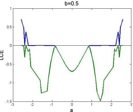
From the Neimark-sacker bifurcation theorem in [26, 27], the proof is completed. 2 Again, we compute the (LCEs) for system (3.1) via the Householder QR-based method to detect chaos. Figure 2 shows the LCEs for system (2.1) with the initial conditions(xo, yo) = (0.1,0.1). We
[image:12.612.219.449.511.705.2]find that LCE1 =0.7009and LCE2 =0.0038.
4. EXISTENCE OFMARROTO’S CHAOS
In this section, we prove that the system (3.1) is chaotic in the sense of Marrotto [35].
Definition 1 — Let the functionF : Rn → Rnbe differentiable inBr(Z). The pointZ ∈ Rn
is an expanding fixed point ofF inBr(Z), ifF(Z) =Zand all eigenvalues ofDF(X)exceed1in
norm for allX∈Br(Z).
Definition 2 — Assume thatZis an expanding fixed point ofF inBr(Z)for somer >0. ThenZ
is said to be a snapback repeller ofF if there exists a pointX0 ∈Br(Z)withX06=Z, FM(X0) =Z
andDFM(X0)6= 0for some positive integerM.
Firstly, we give the condition thatf ix(0,0)of map (3.1) is an expanding fixed point ofF. For map (3.1),
F(Xn) =
Ã
a(xn−x3n−xny2n) +b(−yn+ynx2n+yn3)
b(xn−x3n−xnyn2) +a(yn−ynx2n−yn3)
!
, Xn= (xn yn)T.
The eigenvalues corresponding with the fixed pointf ix(0,0)are given by
λ1,2= −p(0,0)±
p
p2(0,0)−4q(0,0)
2 ,
where
p(0,0) =−2a,
q(0,0) =a2+b2,
Since the eigenvalues associated with the fixed pointf ix(0,0)are a pair of complex eigenvalues λandλ, and the norm of them exceeds unity, which is equivalent to¯
(
p2(0,0)−4q(0,0)<0, q(0,0)−1>0.
Let
S1(0,0) =p2(0,0)−4q(0,0) =−4b2
ifb >0, then for
−4b2 <0,
we have
b2 >0.
Let
S2(0,0) =q(0,0)−1 =a2+b2−1,
So, we have
a <−ib or a > ib.
Thus,S2(0,0)>0if(a, b)∈D2={(a, b)|a <−ibora > ib}.
In view of the above analysis, we may state the following lemma.
Lemma 6 — If(a, b)∈ D1∩D2 andb > 0, thenp2(0,0)−4q(0,0)<0andq(0,0)−1 >0.
Moveover, if the fixed pointz∗(x∗, y∗)of map (3.1) satisfies
z∗(x∗, y∗)∈Uz∗ ={(x∗, y∗)|x∈D1∩D2, b >0}
thenz∗(x∗, y∗)is an expanding fixed point inUz∗.
According to the definition of a snap-back repeller, one needs to find one pointz1(x1, y1)∈Uz∗ such thatz1 6= z∗, FM(z1) = z∗,|DFM(z1)| 6= 0, for some positive integerM, where MapF is
defined by (3.1).
To proceed, notice that
(
a(x1−x31−x1y12) +b(−y1+y1x21+y13) =x2
b(x1−x31−x1y21) +a(y1−y1x21−y31) =y2
(4.1)
and (
a(x2−x32−x2y22) +b(−y2+y2x22+y23) =x∗
b(x2−x3
2−x2y22) +a(y2−y2x22−y23) =y∗
(4.2)
Now, a mapF2has been constructed to map the pointz1(x1, y1)to the fixed pointz∗(x∗, y∗)after
two iterations if there are solutions different fromz∗for Eqs. (4.1) and (4.2). The solutions different fromz∗for Eq. (4.2) satisfy the following equation
x2= x
∗−by
2(−1+x22+y22)
a(1−x2
2−y22) , y2 = y∗−bx2(1−x22−y22)
a(1−x2
2−y22) .
(4.3)
Substitutingx2andy2 into Eq. (4.1) and solvingx1,y1, we have
x1 = x
∗+by
2(1−x22−y22)
a2(1−x2
2−y22)(1−x21−y21) +
by1
a ,
y1= y
∗−bx
2(1−x22−y22)
a2(1−x2
2−y22)(1−x21−y12)−
bx1
a .
By simple calculations, we get
|DF2(z1)| = [B+
δ
2{−cδy−2A
2B+B(1−A2)}]
× [D− cδ2
2 C+δD(−s+cA)] − [cδy+cδBC+cδ2y(−s+cA)]
× [−δ 2 +
δ
2{−D+δA
2−δ
2(1−A
2)}],
where
A=x1+δ
2(x1(1−x
2
1)−y1), B= 1 +
δ
2(1−3x
2 1)
C=y1+δy1(−s+cx1), D= 1 +δ(−s+cx1).
Obviously, if the condition in Lemma 4 is satisfied, the solutions of Eqs. (4.3) and (4.4) will be farther subject toz1(x1, y1),z2(x2, y2)6=z∗(x∗, y∗),z1(x1, y1)∈Uz∗ and|DF2(z1)| 6= 0, thenz∗ is a snap-back repeller inUz∗. Thus, the following theorem is established.
Theorem 1 — Assume that those conditions in Lemma 4 hold. If
1. δ42(1−3x∗2)2−2cδ2y∗ <0and δ2(1−3x∗2) +cδ22y∗>0,
2. the solutions(x2, y2)and(x1, y1)of Eqs. (4.3) and (4.4) satisfy in addition(x1, y1),(x2, y2)6=
(x∗, y∗),(x
1, y1)∈Uz∗,(x1, y1)6= (0,0)and|DF2(z1)| 6= 0, thenz∗(x∗, y∗)is a snap-back repeller of map (2.1), and hence map (2.1) is chaotic in the sense of Marotto.
5. NUMERICALSIMULATIONS
This part is concerned with numerical simulations of Eq. (1.1) in both casesρbeing real and complex. First of all, to reveal the qualitative dynamical behaviors of system (2.1), we present a complete bifurcation sequence that is observed for different values ofρ.
As shown in Figure 3, when plotting the bifurcation diagram of xas a function of ρ, the fixed pointf ix1(0,0)losses stability atρ = −1and a stable periodic solution of period 2 appears and as
ρdecreases, the periodic solution of period 2 losses its stability. The numerical simulations shows that the period-doubling bifurcation may continue and go to chaos. The initial condition taken here is (x0, y0) = (0.1,0.1). In order to explore a larger portion of the behavior of system (2.1), we
are interested in plotting the bifurcation diagram of|z|as a function ofρ. Figure 4 shows that the region of stability of the fixed pointf ix1(0,0)is the same as forx versusρ. Atρ = 1, f ix1(0,0)
4 becomes unstable, and a periodic solution of period 8 appears and chaos happens. Second of all, to reveal qualitative dynamics of system (3.1), we fix the parameterb = 0.5, and assume that the parameterais free. Now we give the specific values of the parameter in system (3.1). Letb = 0.5 andarange from0.8to2.5, then system (3.1) becomes
xn+1 = a(xn−x3n−xnyn2) + 0.5(−yn+ynx2n+yn3),
[image:16.612.115.562.197.458.2]yn+1 = 0.5(xn−x3n−xnyn2) +a(yn−ynx2n−y3n).
Figure 3: Bifurcation diagram of system (2.1): xvs.ρ.
Figure 4: Bifurcation diagram of system (2.1): |z|vs.ρ.
After simple calculations, one may discover that system (3.1) generates an invariant circle (quasi-period orbit) while parameteragoes through0.9, which is the Neimark-Sacker bifurcation value of map (3.1) as shown in Figure 10. In fact, the Jacobian matrix of map (3.1) has a pair of complex conjugate eigenvalues: λ1,2 = a±0.5iand we can see that d(da|λ|)|0.9 6= 0, and λn(−1)|0.9 6= 1,
Figure 5: Bifurcation diagram of system (3.1): xvs.a.
Figure 6: Bifurcation diagram of system (3.1): |z|vs.a.
Figure 7: Bifurcation diagram of system (3.1):xvs.a.
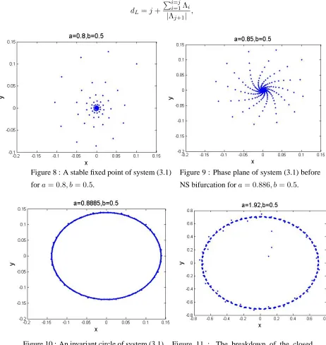
[image:17.612.130.417.330.569.2]to measure the fractal dimension of a chaotic attractor, here we use Lyapunov dimension proposed by Kaplan and York [30, 31]. The fractal Lyapunov dimension of a chaotic attractor is given by [32]
dL=j+
Pi=j
i=1Λi
[image:18.612.102.564.166.654.2]|Λj+1| ,
Figure 10 : An invariant circle of system (3.1) fora= 0.9, b= 0.5.
Figure 11 : The breakdown of the closed invariant circle of system (3.1) for a = 1.98, b= 0.5.
Figure 8 : A stable fixed point of system (3.1) fora= 0.8, b= 0.5.
Figure 12 : Chaotic attractor of system (3.1) fora= 2.3, b= 0.5.
Figure 13 : Chaotic attractor of system (3.1) fora= 2.5, b= 0.5.
whereΛ are Lyapunov exponents such thatΛ1 ≥ Λ2... ≥ Λn, j is the largest integer such that
Pi=j
i=1Λi ≥0, and
Pi=j+1
i=1 Λi ≤ 0. Now for system (3.1), since we have fora= 1.9, andb = 0.5, Λ1 = 0.0021andΛ2 =−0.5654, thendl= 1 + 00..00215654 = 1.0035. So, system (3.1) exhibits a fractal
structure, this can be shown in Figure 14.
6. CHAOSCONTROL
[image:19.612.179.418.446.652.2]The problems of control of chaos attract attention of the researchers and engineers since the early 1990’s; the state of the art of controlling chaotic systems is presented in recent books [33, 34].
Roughly speaking, there are two kinds of ways to control chaos: feedback control and non-feedback control. The frame of a chaotic attractor is given by infinitely many unstable periodic orbits. The task is to use the unstable periodic orbits to control chaos. In this paper, we apply the Ott-Grebogi-Yorke method which uses this fact. Consider the unstable periodic orbit Xp,i ∈ Rn withi = 1,2, ...., p,
wherepis the period length. Consider the parameterized system
Xn+1=f(Xn, ρn).
By changing ρn slightly, the periodic points are also shifted slightly. That is, Xp,i(ρn) fori = 1,2, ...., p. We describe the method as applied to the stabilizing of period one orbits (i.e. fixed points) of the map (2.1).
Let X∗(ρ)denote an unstable fixed point on the attractor. For values ofρclose toρ0 and in the
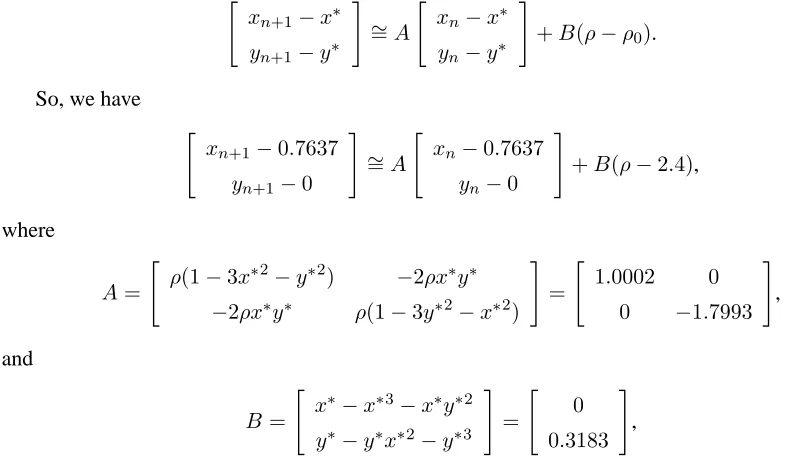
neighborhood of the fixed point X∗(ρ0)the map can be approximated by the linear map Xn+1−X∗(ρ0) =A[Xn−X∗(ρ0)] +B(ρ−ρ0),
whereAis ann×njacobian matrix andB is ann−dimensional column vector given in the form
A:=Dxf(X, ρ), B:=Dρf(X, ρ).
We introduce the time-dependence of the parameterρby assuming that it is a linear function of the variable Xnof the form
ρ−ρ0 =−KT(Xn−X∗(ρ0)).
The1×nmatrixKT is to be determined so that the fixed point X∗(ρ0)becomes stable.
We obtain
Xn+1−X∗(ρ0) = (A−BKT)(Xn−X∗(ρ0)).
Which shows that the fixed point will be stable provided that then×nmatrixA−BKT is a asymptotically stable, i.e., all its eigenvalues have modulus less than one.
In this part we will control the chaotic behavior of system (2.1), that isρis real. Now we fix the parameterρ = 1.45such that the system (2.1) is chaotic. We takeρas the control parameter which is restricted to lie in a small interval|ρ−ρ0|< δ,δ >0, around the nominal valueρ0 = 1.45. The
system (2.1) becomes
f :xn+1 =2.4(xn−x3n−xnyn2),
g:yn+1 =2.4(yn−ynx2n−yn3).
We consider the stabilization of the unstable period one orbitf ix2 = (x∗, y∗) = (0,
q
ρ−1 ρ ). At
ρ= 2.4,f ix2becomesf ix2 = (0,0.7637). The map (6.1) can be approximated in the neighborhood
of the fixed point by the following linear map
"
xn+1−x∗ yn+1−y∗
#
∼ =A
"
xn−x∗ yn−y∗
#
+B(ρ−ρ0).
So, we have
"
xn+1−0.7637
yn+1−0
#
∼ =A
"
xn−0.7637
yn−0
#
+B(ρ−2.4),
where
A=
"
ρ(1−3x∗2−y∗2) −2ρx∗y∗ −2ρx∗y∗ ρ(1−3y∗2−x∗2)
#
=
"
1.0002 0 0 −1.7993
#
,
and
B =
"
x∗−x∗3−x∗y∗2
y∗−y∗x∗2−y∗3
#
=
"
0 0.3183
#
,
If we letKT = (k1, k2). Then the linearized map becomes
"
xn+1−x∗
yn+1−y∗
#
∼
= (A−BKT)
"
xn−x∗
yn−y∗
#
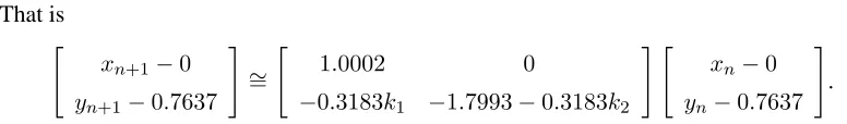
[image:21.612.73.467.185.417.2].
That is
"
xn+1−0
yn+1−0.7637
#
∼ =
"
1.0002 0
−0.3183k1 −1.7993−0.3183k2
# "
xn−0
yn−0.7637
#
.
The eigenvalues of the matrixA−BKT can be obtained by solving the characteristic equation
|A−BKT −γI|= 0,
which givesγ1 =−1.7993−0.3183k2andγ2= 1.0002. Generally speaking, we must choose values
[image:22.612.129.517.124.181.2]fork1 andk2 such that γ1γ2 < 1,γ1 < 1andγ1 > −1. So, we have−8.7930 < k2 < −2.5112.
Figure 15 shows the controled fixed point of system (6.1) fork1 = 4.
In the same manner, we can control chaos in caseρ is complex which is ommitted here for no repetition.
7. CONCLUSION
In this paper, we have considered a discrete logistic-type equation with complex variables in two different cases of the control parameterρin the defining equation: real and complex. Our theoretical analysis and numerical simulations have demonstrated that the map undergoes pitchfork bifurcation, flip bifurcation, Neimark-Sacker bifurcation and chaos. Moreover, we have proven that the map in the real case is chaotic in the sense of Marotto. In addition, it has been shown that the map with complex parameterρ demonstrated a fractal structure. Finally, we have applied the OGY feedback control technique to control chaos in caseρ is real. It has been investigated that considering the control parameterρto be complex led to more richer dynamics.
REFERENCES
2. E. A. Jackson and A. Hiiblcr, Periodic entrainment of chaotic logistic map dynamics, Physica D, 44 (1990), 404-420.
3. S. J. Linz and M. Lticke, Effect of additive arid multiplicative noise on the first bifurcations of thelogistic map, Phys. Rev. A, 33 (1986), 2694-2703.
4. Y. Yamaguchi and K. Sakai, New type of crisis showing hysteresis, Phys. Rev. A, 27 (1983), 2755-2758. 5. A. C. Fowler, M. J. McGuinness, and J. D. Gibbon, The complex Lorenz equations, Physica D, 4(2)
(1982), 139-163.
6. G. M. Mahmoud, E. E. Mahmoud, and M. E. Ahmed, A hyperchaotic complex Chen system and its dynamics, International Journal of Applied Mathematics & Statistics, 12(D07) (2007), 90-100. 7. G. M. Mahmoud, Periodic solutions of strongly non-linear Mathieu oscillators, International Journal of
Non-Linear Mechanics, 32(6) (1997), 1177-1185.
8. G. M. Mahmoud and S. A. Aly, Periodic attractors of complex damped non-linear systems, International Journal of Non-Linear Mechanics, 35 (2000), 309-323.
9. G. M. Mahmoud, Stability regions for coupled Hill’s equations, Physica A, 242 (1997), 139-149. 10. G. M. Mahmoud, On the generalized averaging method of a class of strongly nonlinear forced oscillators,
Physica A, 199 (1993), 87-95.
11. R. A. Holmgren, A first course in discrete dynamical systems, Second Edition, Springer-Vcrlag, (1996). 12. G. M. Mahmoud, Bountis Tassos, G. M. Abd El-Latif, and E. E. Mahmoud, Chaos synchronization of
two different chaotic complex Chen and Lu¨systems, Nonlinear Dyn., 55 (2009), 43-53.
13. C. Z. Ning and H. Haken, Detuned lasers and the complex Lorenz equations: Subcritical and supercriti-cal Hopf bifurcations, Phys. Rev. A, 41 (1990), 3826-3837.
14. Yong Xu, Wei Xu, and G. M. Mahmoud, On a complex duffing system with random excitation, Chaos, Solitons and Fractals, 35 (2008), 126-135.
15. A. A. ElSadany and A. M. A. El-Sayed, On a complex logistic difference equation, International Journal of Modern Mathematical Sciences, 4(1) (2012), 37-47.
16. A. M. A. El-Sayed and S. M. Salman, Dynamic behavior and chaos control in a complex riccati-type map, Quaestiones Mathematicae (2015), DOI: 10.2989/16073606.2015.1115441.
17. R. P. Agarwal, Difference equations and inequalities, New York, NY, USA, second edition, 2000. 18. S. Elaydi, An introduction to difference equations, third edition, Springer Verlag, New York, 2005. 19. S. Elaydi, Is the world evolving discretely?, Adv. in Appl. Math., 31(1)(2003), 19.
20. R. Holmgren, A first course in discrete dynamical systems, Second Edition, Springer Verlag, New York, 1996.
21. W. G. Kelley and A. C. Peterson, Difference equations, an introduction with applications, Second Edi-tion, Academic Press, New York, 2000.
22. V. L. Kocic and G. Ladas, Global behavior of nonlinear difference equations of higher order with appli-cations, Kluwer Academic Publishers, Dord recht, 1993.
24. J. Guckenheimer and P. Holmes, Nonlinear oscillations, dynamical systems, and bifurcations of vector fields, Springer-Verlag. New York, 1997.
25. E. Ott, Chaos in dynamical systems, Cambridge University Press, Cambridge, 1993.
26. Y. A. Kuznetsov, Elements of applied bifurcation theory, applied mathematical sciences, V. 112. Springer, New York, third edition, 2004.
27. S. Wiggins, An introduction to applied nonlinear dynamics and chaos, New York: Springer-Verlag, 1990.
28. F. E. Udwadia and H. von Bremen, A note on the computation of the largestp-Lyapunov characteristic exponents for nonlinear dynamical systems, J. Appl. Math. Comput., 114 (2000), 205-214.
29. Albers; Alexanderson, Benoit Mandelbrot: In his own words, Mathematical people : Profiles and inter-views, (2008). Wellesley, Mass: AK Peters, p. 214. ISBN 978-1-56881-340-0.
30. V. I. Oseledec, A multiplicative ergodic theorem: Lyapunov characteristic numbers for dynamical sys-tems, Trans. Moscow Math. Soc., 19 (1908), 197-231.
31. J. L. Kaplan and Y. A. York, A regime observed in a fluid flow model of Lorenz, Comm. Math. Phys., 67 (1979), 93-108.
32. J. H. E. Cartwright, Nonlinear stiffness, Lyapunov exponents, and attractor dimension, Phys. Lett. A, 264 (1999), 298-304.
33. G. Chen and X. Dong, From chaos to order: Methodologies, perspectives and applications, world scientific, (1998).
34. H. G. Schstcr, Handbook of chaos control, Wiley-VCH, (1998).