Multi-view Orientation Estimation using Bingham Mixture Models
Sebastian Riedel, Zoltan-Csaba Marton, Simon Kriegel
Institute of Robotics and Mechatronics, German Aerospace Center (DLR), 82234 Oberpfaffenhofen, Germany Email:{firstname.lastname}@dlr.de
Abstract—This paper describes a multi-view pose estimation system, that is exploiting the mobility of a depth sensor through mounting it onto a robotic manipulator. Given a pose estimation algorithm that performs feature extraction and matching to a model database, we investigate the probabilistic modeling of the pose space as well as the measurement uncertainty, to be used in a sequential state estimation approach.
Uncertainties in 3d position can be modeled in a parametric way by 3d Gaussians, but the space of rotations in 3d - the special orthogonal group SO(3) - requires approaches from directional statistics. A convenient representation for orientations are unit quaternions over which the Bingham distribution defines a para-metric probability density function. The Bingham distribution also correctly accounts for the sign symmetry of orientation quaternions and leave degrees of freedom unconstrained (which is especially useful if an object is rotationally symmetric, with no unique quaternion describing its orientation).
In our experiments we test different sequential fusion methods, optimize their parameters, and investigate how the derived filter performs in a case with high uncertainties.
I. MOTIVATION
Recognition and pose estimation of known objects is nec-essary for many tasks including monitoring and tracking pur-poses or robotic manipulation of objects. Whereas recognition is the task of deciding which object is present, pose estimation refers to estimating an object’s position and orientation in up to three dimensions. If the objects are known in advance, ana-lyzed by the estimation algorithm in an offline training phase and the online application is limited to the a priori known objects, one speaks of model based object recognition and pose estimation. Robotic part handling in industrial applications is a prominent example and commercial use case for such algorithms as industrial manipulation is usually limited to a fixed set of parts known in advance.
Model based recognition and pose estimation have been sub-ject to extensive research since the early 70s [1] and generally work in two steps. In the offline phase, a representation of the object is built using features derived from training data. In the online phase, incoming sensor data is matched to this represen-tation and by doing so, the desired quantity - for example the object’s pose - is measured. The quality of this measurement is affected through several aspects of the measurement process. Aspects involving the sensor directly include for example the inherent loss of 3d information when working with monocular 2d intensity images, loss of color information in 3d range data, limited spatial and temporal resolution, limited field of view and sensor noise. The sensed data is affected by its environment for example by scene illumination and occlusions. Lastly, the objects to be recognized and located can share
feature characteristics with the environment, among each other or among different views of the same object. This last aspect can lead to classification and pose ambiguities even under perfect environment and noise free sensing conditions.
Aforementioned influences are minimized by designing the extracted features to be more or less invariant to many of these aspects. This way, state-of-the-art algorithms achieve correct recognition results and pose measurements using only a single view of the scene or object. In case of ambiguities or inaccuracies introduced by the environment, the object itself or simply sensor noise, it can be helpful to acquire several sensor measurements and fuse the information obtained by them [2]. Utilizing multiple measurements in general will lead to higher accuracy of the measured quantities. Furthermore, tasks for which the presence of unknown objects is expected often necessitate fusing information from multiple measurements to obtain reliable estimates (for example in object search or scene exploration as explained in [3]). It is therefore purposive to employ approaches based on multiple views for scenarios, environments or objects where large inaccuracies are to be expected.
In this paper, we present an approach for estimation the object orientation applying multiple views using a Bingham Mixture Model (BMM).
II. SEQUENTIALORIENTATIONESTIMATION USING
BINGHAMMIXTUREMODELS
This section reviews the Bingham distribution over unit quaternions and describes the formalism and two implementa-tions for sequentially estimating an object’s orientation using Bingham Mixture Models as probabilistic representation.
A. The Bingham Distribution over Unit Quaternions
The Bingham distribution is a distribution over n-dimensional hyperspheres Sn, n ∈ N+ [4]. The distribution is always antipodally symmetric, thus in the case of n= 3, it correctly captures the antipodal symmetry of the quaternion parametrization of rotations in 3d. The Bingham distribution over quaternions is derived from a 4d zero-mean Gaussian density p(x∗;C) =p 1 (2π)4|C|exp Å −1 2x ∗T C−1x∗ ã (1) where x∗ ∈R4 and C is a covariance matrix. This standard
Gaussian is defined over all R4 and by re-normalizing it
we can obtain a proper probability distribution over S3 and
thus 3d rotations. Intuitively, the process of renormalization
can be thought of as intersecting the unit quaternion sphere with the volumetric Gaussian density in 4d and normalizing the resulting density on the sphere to integrate to one. The Gaussian form of the Bingham distribution is thus
p(x;C) = 1 F exp(x
TC−1x) (2)
withx∈S3 is now constrained to lie on the unit sphere and F is chosen so that
Z
x∈S3
exp(xTC−1x) = 1 (3) The standard form of the Bingham distribution is given by
B(x;K, V) := 1 F(κ1, κ2, κ3) exp 3 X i=1 κi(viTx) 2 ! (4)
withK= (κ1, κ2, κ3)T, κi∈R−∪ {0} denoting the concen-tration parameters,V = [v1|v2|v3], vi∈S3a set of orthogonal basis vectors and x ∈ S3 a unit quaternion. The standard
form is based on an eigenvector/eigenvalue decomposition of the Gaussian covariance matrix C, zero-ing out κˆ4 and
imposing an ordering constraint on the eigendecomposition. By choosing the eigenvectors vi, i ∈ {1,2,3} one adjusts the rotation axis in which rotational uncertainty applies. By choosing the concentration parameters, the kind of rotational uncertainty is specified. Two easy interpretable choices are:
• κ1 = κ2 = κ3 = α ≤ 0: Gaussian-like rotational
uncertainty. For α = 0 the distribution is completely uniform. The more negative theαgets, the more peaked the distribution gets around its mode v4 where v4 is
uniquely defined (orthonormal completion) byhv4, vii= 0;i= 1,2,3.
• κ1 = κ2 κ3 ≤ 0: Increasing the value of κ3 leads
to increased uncertainty of the 4d-Gaussian in the prin-cipal component direction v3. Setting the concentration
parameterκ3 to zero results in an infinite variance along
the direction v3 for the 4d Gaussian and in terms of
the normalized distribution over rotations this results in a density function mimicking a great circle on the unit quaternion sphere. When v3 has the special form
of v3 = (0, a, b, c) this axis around which the uniform
rotation occurs is exactly(a, b, c).
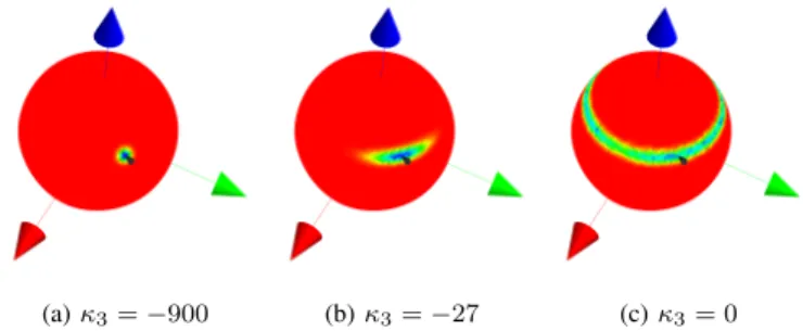
In Figure 1 the rotational uncertainty for different values of κ3 ∈ {−900,−480,0} and v3 = (0,0,0,1) is shown
and the increase in uncertainty for rotations around (0,0,1)
is clearly visible. The plots shown are similar in nature to EGI (extended Gaussian image) plots and an intuitive way to visualize probability distributions over rotations. They work by rotating a base point on the sphere by many sampled rotations of the distribution. At the rotated point’s location, a counter is increased. When visualizing the counts via a heat map, this gives a visualization of how the distribution behaves. In the plots in Figure 1 the pointp= (1,1,1)/||(1,1,1)|| is rotated byn= 100000sampled rotations. The mode of the distribu-tion is the identity rotadistribu-tion, hence forκ3<0the peak is atp.
(a)κ3=−900 (b)κ3=−27 (c)κ3= 0
Fig. 1: EGI plots (see text for details) showing the effect of different concentration parameters κ3. Increasingκ3 leads to
increased rotational uncertainty around the z-axis.
Forκ3= 0, we see the expected rotational invariance around
the z-axis which is a consequence of choosingv3= (0,0,0,1).
The major problem with using the Bingham distribution in practice is the normalization constant F(κ1, κ2, κ3)which
is expensive to compute [5]. Glover therefore precomputes the normalization constant for a discrete set of concentrations parameters ranging inκi∈[−900,0]and interpolates them as necessary.
B. Bingham Mixture Models
While individual Bingham distributions are in general uni-modal (except one or more concentration parameters are zero), a sum of several Binghams can represent arbitrary probability landscapes over rotations given a sufficient number of components. Formally, a Bingham Mixture Model (BMM) is defined as
BMM(x;{αi},{Ki},{Vi}) :=X
i
αiB(x;Ki, Vi) (5) whereB(x;Ki, Vi)is Bingham distributed as defined in equa-tion (4) and P
iαi = 1. Unfortunately, BMMs - just like Gaussian mixture models - lose some of their analytical ben-efits as operations like maximum likelihood parameter fitting, entropy calculation and Kullback-Leibler (KL) divergence calculation are not defined analytically anymore and have to be approximated using for example Monte-Carlo integration techniques. In the context of this paper, we need to be able to fit BMMs to quaternion samples, multiply two BMMs and extract the maximum mode of a BMM. For fitting a BMM to a sample set of quaternions {qi}, Glover [6] describes a greedy sample consensus method. The multiplication of two BMMs is done by pairwise multiplication of the Binghams of both mixtures. As the result of multiplying two Bingham distributions is again a Bingham and can be done in an alge-braic way, multiplication of two BMMs is also well-defined. Finding the maximum mode of a BMM cannot be done in closed form. An approximation is computed by sampling a high number of rotations from the BMM (typically 50000), evaluating their probability density value under the BMM and selecting the sample with the maximum value. This procedure will be used in later sections whenever the MAP estimate of a
BMM belief distribution is computed. For sampling a Bingham distribution, Glover [5] introduces an efficient Metropolis-Hastings sampler with the projected 4d-Gaussian density as proposal distribution.
C. Sequential Orientation Estimation using BMMs
The state estimation problem for sequentially estimating an object rotation using Bayes’ theorem can be written as
p(qt|zt, . . . , z0)∝p(zt|qt)p(qt|zt−1, . . . , z0) (6)
whereqt, zt∈SO3are 3d rotations which are without loss of generality assumed to describe an object’s rotation (frameo) in the world framew(qt:=wqo,tresp.zt:=wzo,t). Equation (6) does not contain a dynamic model as found in typical state estimation formulations as for our use case of rotation estimation of objects for industrial robotic manipulation we can assume static objects and precise robot motions. The measurement process underlyingp(zt|qt)can be described as producing a rotation measurements
zt=wt◦qt (7)
based on the object’s rotation qt corrupted by a Bingham mixture distributed independent measurement noise wt ∼
BMM(α,K,V) with ◦ denoting quaternion multiplication. Based on findings of Glover [5], the conditional distribution p(zt|qt)is Bingham mixture distributed according to zt|qt∼
BMM(zt;α,K,V ◦qt)whereV ◦qtare the eigenvectors of the original Bingham mixture components rotated by the fixed qt. This mixture is a distribution overzt given a fixedqt. To apply this model in practice we can rewrite the distribution to obtain one overqtgiven a fixedztby reordering the terms in the same way as presented in [5]
BMM(zt;α,K,V ◦qt) = (8) N X i=1 αi 1 Fi exp 3 X j=1 κi((vi◦qt)Tzt)2 ! = (9) N X i=1 αi 1 Fi exp 3 X j=1 κi((vi−1◦zt)Tqt)2 ! = (10) BMM(qt;α,K,V−1◦zt) (11) If we now assume a Bingham mixture prior p(qt|zt−1, . . . , z0) = BMM(qt;β,K∗,V∗), the posterior is also Bingham mixture distributed by multiplying the prior and measurement BMM. The components of the posterior BMM are built by pairwise multiplication of the prior and measurement mixture components
p(qt|zt, . . . , z0) = (12) N X i=1 M X j=1 αiβjB(qt;Ki, Vi−1◦zt)B(qt;Kj∗, V ∗ j) (13) As the multiplication of two Binghams is well-defined, Equation (13) describes a unique algebraic solution to this sequential estimation problem.
1) Fusion based on Mixture Reduction: In the algebraic posterior defined by Equation (13) we see that for a prior and measurement distribution with N and M components the resulting posterior mixture will have N ×M components. To avoid a rapidly increasing number of components with every estimation step, mixture reduction strategies can be used to reduce the number of components while maintaining an acceptable level of representational accuracy with respect to the unreduced mixture. For the evaluation of our sequential Bingham mixture fusion, the reduction method of Runnalls [7], originally developed for Gaussian mixtures, has been implemented and tested for Bingham mixtures. It works by iteratively choosing two components of the mixture and merg-ing them into one component. This is done until a specified number of components is reached. The two components to be merged are chosen by an upper bound criteria derived by Runnalls. It states that the the KL divergence of the mixture before the merge ( Mi+j ) and after the merge ( Mij ) of components iandj is smaller than
dkl(Mi+j,Mij)≤αidkl(Bi, Bij) +αjdkl(Bj, Bij) (14) withBi andBj denoting the individual original components,
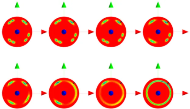
Bij denoting the merged component and αi, αj are the re-spective components’ weights. As Bi,Bj andBij are single Gaussians (or Binghams), the KL divergence is analytically computable. Every iteration step, the two components leading to a minimal approximated before-after KL divergence are chosen to be merged. An example reduction is illustrated in Figure 2 by reducing an eight component mixture gradually down to one component.
The final algorithm for state fusion based on algebraic multiplication thus has two steps. At first, the full posterior is computed through element-wise multiplication as in equation (13). In the second step, the full posterior is reduced to a predefined maximum number of allowed components Nmax, which is the only parameter of this fusion method. For notational convenience, we denote this fusion algorithm as multiply & reduce (M+R) method.
2) Fusion based on Sequential Monte-Carlo Sampling: A different way to compute the posterior distribution was imple-mented using a standard sequential Monte Carlo (SMC) ap-proach. In this approach, the posterior is represented by a set of M equally weighted samples{qm
t }, m= 1, . . . , Mdistributed according to the posterior distribution{qm
t } ∼p(qt|z0, . . . , zt) [8]. The standard importance weighting and resampling steps are implemented by evaluation the measurement model mea-surement model p(zt|qt) [8] and drawing samples from the weighted set with replacement and proportional to the weights. To allow the sample set to change ”position”, a Bingham mixture is fitted to the posterior sample set using the method described in [6] and sampled again in order to obtain the prior sample set for the next time step. The main parameter of the SMC method for state fusion is the number samples M. In all experiments later onM = 100000, which provides a good balance between computation time an representational accuracy.
Fig. 2: EGI plots illustrating the implemented Bingham mix-ture reduction: The initial Bingham mixmix-ture (top,left) has eight components and roughly represents a 4-fold symmetric distribution around the z-axis (two components per fold). From left to right, top to bottom, the mixture gradually gets reduced by one component.
III. EXPERIMENTS
We evaluated the presented sequential BMM fusion methods over a range of parametrizations in two test scenarios dealing with the orientation estimation of real world objects for robotic grasping and manipulation.
In experiment III-A, test data from a previous experiment of our group has been reused [9]. The test data contains object pose measurement sequences over multiple views for three industrial objects. In this experiment, the obtained results using BMM fusion are compared to previous results from [9].
The second experiment, III-B, was chosen to evaluate ori-entation estimation under significantly higher uncertainty. It is based on a less sophisticated method for object orientation estimation which necessitates a more complex BMM measure-ment model. In this experimeasure-ment, the theoretical minimum for estimating a unique object orientation due two uncertainty in the measurement process is two sequence views.
Both experiments are based on real sensor data collected using a 6 DoF industrial robot, the Kuka KR16-2, with a mounted Asus Xtion as in [3].
A. Sequential Orientation Estimation under Moderate Uncer-tainty Conditions
For this experiment the test data contains three object pose measurement sequences corresponding to three indus-trial objects (valve, filter and control). The measured object poses were obtained using the object recognition and pose estimation method from [3] with an average rotational error of around four degrees. All sequences contain 20 views of their object from different viewing directions and all views lead to successful detection, hence 20 rotation measurements zt, t= 1, . . . ,20exist for every object. Whereas thevalveand
controlobject have a clear unique pose, the filter object has a strong rotational ambiguity in form of a 4-fold rotational symmetry. It is thus detected with a rotational error of±90◦
or 180◦in 7 out of the 20 views.
Two Bingham mixture measurement models have been defined for evaluation of the test sequences. The first one is the simple uninformed standard model where we assume the rotation measurement results from the correct pose corrupted by small Gaussian-like noise. A measurement model p(zt|qt) describing this noise characteristic is created by rotating the correct pose by a Bingham with mode at identity and concen-tration parameters specifying a small Gaussian-like deviation, specifically K=κ Ñ 1 1 1 é V= 0 0 0 1 0 0 0 1 0 0 0 1 (15) p(zt|qt) =B(zt;K,V ◦qt) (16) To deal with outliers, a uniform Bingham Buni(zt) = B(zt; (0,0,0),V) is added to the measurement model. This results in the Bingham mixture model
pG(zt|qt) =α1B(zt;K,V ◦qt) +α2Buni(zt) (17) which can be ”inverted” to a distribution overqtby following equations (8) to (11). The Gaussian measurement model pG has two parameters: the measurement concentrationκand the outlier ratio α= (α1, α2). This measurement model will be
used for all three objects.
To test a more complex measurement model, thefilterobject was additionally evaluated with a measurement model taking the 4-fold symmetry around the object’s z-axis into account. It is based on a five component Bingham mixture model. The first four components describe rotations of{0,+90,−90,180} degrees of the correct pose qt around the symmetry axis and the fifth component again a uniform distribution. Construction of the symmetric measurement model pS is a straightfor-ward extension of equation (17) by adding the symmetric components. The resulting parameters for the model pS are again the measurement concentrationκused for the first four components and the component weighting α= (α1, . . . , α5).
The metric for comparing different parameter settings for the measurement models {pG, pS}and state fusion strategies {SMC,M+R} is based on the maximum a posteriori (MAP) rotation error with respect to the ground-truth orientation averaged over the last ten views of every viewing sequence and all three viewing sequences.
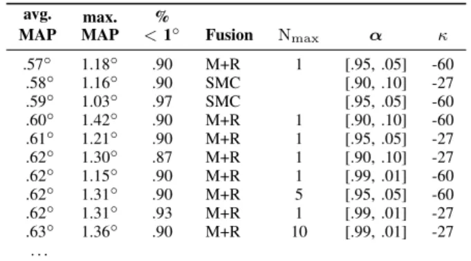
For the Gaussian-like measurement modelpG the evaluated parameter range is listed in Table I. A summary of the top ten parametrizations is given in table II, which also includes the maximum MAP error within the last ten views over all three sequences and the percentages of MAP estimates below one, three and five degrees of error for the last ten views.
Out of the 72 parametrizations, 34 perform very close to the best one with a difference of only0.21◦ in the avg. MAP
error and 0.64◦ in the maximum MAP error. Seven of the
top 34 runs are based on the SMC fusion, 27 are based on M+R. The outlier ratio α does not have an impact on
the obtainable performance, the measurement concentrationκ does. All of the 34 good performing runs have a concentration κ ∈ {−27,−60,−120}, which correspond to 68% of the samples drawn from such a distribution having an rotational deviation smaller than{29◦,19◦,14◦} from the mode of the distribution. This is somewhat contradicting to the actual measurement error in the object sequences, as for thecontrol,
filter and valvesequence 68% of the measurement errors lie below 4.4◦, 6.9◦ and 4.4◦. Thus even a concentration value
of κ = −240 resp. 9.8◦ for the 68% interval encloses the measurement uncertainty well enough.
Figure 3 shows the MAP error evolution of the best SMC and M+R method compared to the error obtained by several other approaches to orientation fusion evaluated in [9] for the
filter object sequence. As can be seen, the Bingham mixture approaches yield competitive results to a particle filter, a pose clustering and a histogram filter approach.
TABLE I: Explored parameter ranges for Gaussian-like measurement model evaluation
Functional
Component Parameter Explored Range
SMC M {100000}
M+R Nmax {1, 5, 10}
pG α {(.9, .1),(.95, .05),(.99, .01)}
κ {−900,−480,−240,−120,−60,−27}
TABLE II: Top 10 parametrizations (avg. MAP error) for the fusion evaluation of the Gaussian-like measurement model.
avg. MAP max. MAP % <1◦ Fusion N max α κ .57◦ 1.18◦ .90 M+R 1 [.95, .05] -60 .58◦ 1.16◦ .90 SMC [.90, .10] -27 .59◦ 1.03◦ .97 SMC [.95, .05] -60 .60◦ 1.42◦ .90 M+R 1 [.90, .10] -60 .61◦ 1.21◦ .90 M+R 1 [.95, .05] -27 .62◦ 1.30◦ .87 M+R 1 [.90, .10] -27 .62◦ 1.15◦ .90 M+R 1 [.99, .01] -60 .62◦ 1.31◦ .90 M+R 5 [.95, .05] -60 .62◦ 1.31◦ .93 M+R 1 [.99, .01] -27 .63◦ 1.36◦ .90 M+R 10 [.99, .01] -27 . . .
The evaluation of the multimodal 4-fold symmetric mea-surement model pS was carried out solely based on the test sequence of thefilterobject, as only this object shows this kind of measurement ambiguity (cf. the raw measurement line in the filter subplot of Figure 3). A total of 168 parametrizations has been evaluated exploring combinations of the two fusion methods, with both measurement models pG and pS and parametrizations given in table III.
Out of the 20 measurements in the filter sequence, seven are ±90◦ or 180◦ off, due to the 4-fold symmetry of the filter object. Six of these seven outliers fall into the last ten views of the sequence, over which the avg. MAP error metric is built. This evaluation thus puts special emphasis on how the parametrizations handle this ambiguity. The first 43 parametrizations yield similar performance in terms of average
1 2 3 4 5 6 7 8 9 10 11 12 13 14 15 16 17 18 19 20 Number of views fused
0 1 2 3 4 5 6 7 8 Degr ee
MAP Rotational Error, Obj: Filter
raw measurements SMC M+R Hist PF Cluster
Fig. 3: MAP Rotational Error plots for the best SMC vs. the best M+R parameter settings in comparison to a histogram filter (discretized rotation space, Hist), a particle filter (PF) and a pose clustering approach (Cluster).
TABLE III: Explored parameter ranges for multimodal mea-surement model evaluation
Functional
Component Parameter Explored Range
SMC M {100000} M+R Nmax {1, 5, 10} pG α {(.9, .1),(.95, .05),(.99, .01)} κ {−900,−480,−240,−120,−60,−27} pS α {(.25, .22, .22, .22, .1), (.45, .15, .15, .15, .1), (.65, .08, .08, .08, .1), (.85, .02, .02, .02, .1)} κ {−900,−480,−240,−120,−60,−27}
MAP error (best/worst difference: 0.39◦) and maximum MAP error (best/worst difference: 1.23◦). The first 4-fold symmetric parametrization using a significant weight for the symmetric components (α2...4= 0.15) is ranked 50th with an avg./max.
MAP error of 1.14◦/ 1.37◦. The worst parametrization using pS and the SMC fusion is ranked 85th with an avg./max. MAP error of 5.39◦/ 10.02◦, while the vast majority of pS -parametrizations with M+R fusion at some point return an MAP estimate around one of the outlier measurements and therefore obtain much worse MAP averages and maximum errors of up to≈180◦. It can be concluded, that both fusion methods perform better with the simple Gaussian measurement model and in general, if used with a complex measurement model, the SMC fusion has an advantage over the M+R fusion.
B. Sequential Orientation Estimation using BMMs under High Uncertainty Conditions
In this experiment, we estimate an object’s orientation by means of a probabilistic viewing direction classification. Using a set of training images from 28 different viewing angles distributed across a half-sphere around the object, a classifier is trained in an offline processing step to predict the viewing direction from which an object feature can be observed from. During sequential estimation, the probabilistic predictionp(D|f)over directionsDgiven the featurefis used to build a measurement distribution p(zt|qt). Classifiers have
1 2 3 4 5 6 7 8 9 10 11 12 13 14 15 16 17 18 19 20 Number of views fused
0 20 40 60 80 100 120 140 160 180 Degr ee
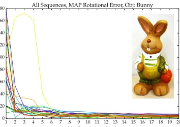
All Sequences, MAP Rotational Error, Obj: Bunny
1 2 3 4 5 6 7 8 9 10 11 12 13 14 15 16 17 18 19 20 Number of views fused
0 20 40 60 80 100 120 140 160 180 Degr ee
All Sequences, MAP Rotational Error, Obj: Mug
Fig. 4: MAP Rotational Error plots for 20 random sequences with 20 views.
been trained for two household objects: a decoration bunny
object and a standard coffee mug. For evaluation, 20 view sequences showing each object from 20 random non-training viewing directions have been recorded.
To fuse this information over multiple views in this ex-periment, the measurement model has to account for two kinds of uncertainties: 1) the uncertainty in the viewing direction classification and 2) for every viewing direction the uniform orientation ambiguity around this viewing axis. The second uncertainty arises for example when using the popular Viewpoint Feature Histogram [10] or similar view-classification systems. We use a Bingham mixture model similar to the symmetric measurement model in experiment III-A to capture both uncertainties in a principled way. The measurement model contains 28 components, one component for every possible viewing direction. Every single component models the rotational invariance about its specific view axis by specifying v3 appropriately, setting the corresponding κ3
to 0 and the remainingκ-s to −27 for the bunny and−120
for themugsequences.
In this experimental setup, using a only a single view of the
object means the orientation of it can only be estimated up to the rotational invariance around the camera optical axis (even if the viewing direction classification is 100% sure that we see it from a specific direction). For a unique orientation estimate, the sequential estimation requires at least two views from two non-parallel viewing directions. Based on the experience of the previous experiment, the SMC fusion implementation with M = 100000samples has been used for this experiment.
Calculating the average MAP error over the last ten views as in experiment III-A (over all 20 sequences per object), the rotation estimation converges to an average error of4.74◦ for the bunny and 9.08◦ for the mug. Figure 4 shows the MAP error evolution for every view sequence. While the resulting errors are too high to be of immediate practical use for robotic applications, the experiment showcases the successful infor-mation fusion of highly uncertain and ambiguous orientation estimates.
IV. CONCLUSION
We presented a sequential BMM-based orientation fusion for multi-view object pose estimation. Two variants of the method are evaluated for different parametrizations, and ap-plied in two cases for orientation estimation of real world objects. We obtained competitive results to other approaches, and were able to significantly improve on the individual detections even on datasets where traditional methods would fail due to the high and non-Gaussian uncertainties.
V. ACKNOWLEDGMENTS
This work has partly been supported by the Euro-pean Commission under contract number H2020-ICT-645403-ROBDREAM.
REFERENCES
[1] R. T. Chin and C. R. Dyer, “Model-Based Recognition in Robot Vision,”
ACM Computing Surveys (CSUR), vol. 18, no. 1, 1986.
[2] S. D. Roy, S. Chaudhury, and S. Banerjee, “Active recognition through next view planning: a survey,”Pattern Recognition, vol. 37, no. 3, pp. 429–446, 2004.
[3] S. Kriegel, M. Brucker, Z.-C. Marton, T. Bodenm¨uller, and M. Suppa, “Combining Object Modeling and Recognition for Active Scene Explo-ration,”IEEE/RSJ IROS, 2013.
[4] C. Bingham, “An Antipodally Symmetric Distribution on the Sphere,”
The Annals of Statistics, 1974.
[5] J. Glover and L. P. Kaelbling, “Tracking 3-D Rotations with the Quaternion Bingham Filter,” MIT, Tech. Rep., 2013. [Online]. Available: http://dspace.mit.edu/handle/1721.1/78248
[6] J. Glover, G. Bradski, and R. B. Rusu, “Monte Carlo pose estimation with quaternion kernels and the bingham distribution,”Robotics: Science and Systems, 2012.
[7] A. R. Runnalls, “Kullback-Leibler Approach to Gaussian Mixture Re-duction,”IEEE TAES, vol. 43, no. 3, pp. 989–999, Jul. 2007. [8] S. Thrun, W. Burgard, and D. Fox,Probabilistic Robotics. MIT Press,
2005.
[9] Z.-C. Marton and S. T¨urker, “On Bayesian Inference for Embodied Perception of Object Poses,” inIEEE/RSJ IROS: Workshop on Metrics of Embodied Learning Processes in Robots and Animals, 2013. [Online]. Available: http://elib.dlr.de/90326/1/bayesian.pdf
[10] R. B. Rusu, G. Bradski, R. Thibaux, and J. Hsu, “Fast 3D recognition and pose using the Viewpoint Feature Histogram,”IEEE/RSJ IROS, Oct. 2010.