White Rose Research Online URL for this paper: http://eprints.whiterose.ac.uk/133889/
Version: Accepted Version Article:
Muthusamy, M., Wani, O., Schellart, A. et al. (1 more author) (2018) Accounting for
variation in rainfall intensity and surface slope in wash-off model calibration and prediction within the Bayesian framework. Water Research, 143. pp. 561-569. ISSN 0043-1354 https://doi.org/10.1016/j.watres.2018.06.022
Article available under the terms of the CC-BY-NC-ND licence (https://creativecommons.org/licenses/by-nc-nd/4.0/).
[email protected] https://eprints.whiterose.ac.uk/ Reuse
This article is distributed under the terms of the Creative Commons Attribution-NonCommercial-NoDerivs (CC BY-NC-ND) licence. This licence only allows you to download this work and share it with others as long as you credit the authors, but you can’t change the article in any way or use it commercially. More
information and the full terms of the licence here: https://creativecommons.org/licenses/
Takedown
If you consider content in White Rose Research Online to be in breach of UK law, please notify us by
1
Accounting for variation in rainfall intensity and surface
1
slope in wash-off model calibration and prediction within
2
the Bayesian framework
3
Manoranjan Muthusamy1,2, Omar Wani3,4, Alma Schellart1 and Simon Tait1
4
1 Department of Civil and Structural Engineering, University of Sheffield, Sheffield, UK
5
2 (At present) School of Water, Energy and Environment, Cranfield University, Cranfield, UK
6
3 Institute of Environmental Engineering, Swiss Federal Institute of Technology (ETH), Zürich, Switzerland
7
4 Swiss Federal Institute of Aquatic Science and Technology (Eawag), Dübendorf, Switzerland
8
Correspondence to: Manoranjan Muthusamy ([email protected])
9
Abstract
10
Exponential wash-off models are the most widely used method to predict sediment wash-off 11
from urban surfaces. In spite of many studies, there is still a lack of knowledge on the effect of 12
external drivers such as rainfall intensity and surface slope on the wash-off prediction. In this 13
study, a more physically realistic “structure” is added to the original exponential wash-off 14
model (OEM) by replacing the invariant parameters with functions of rainfall intensity and 15
catchment surface slope, so that the model can better represent catchment and rainfall 16
conditions without the need of lookup table and interpolation/extrapolation. In the proposed 17
new exponential model (NEM), two such functions are introduced. One function describes the 18
maximum fraction of the initial load that can be washed off by a rainfall event for a given slope 19
and the other function describes the wash-off rate during a rainfall event for a given slope. The 20
parameters of these functions are estimated using data collected from a series of laboratory 21
experiments carried out using an artificial rainfall generator, a 1 m2 bituminous road surface 22
and a continuous wash-off measuring system. These experimental data contain high temporal 23
2
resolution measurements of wash-off fractions for combinations of five rainfall intensities 1
ranging from 33-155 mm/hr and three catchment slopes ranging from 2-8 %. Bayesian 2
inference, which allows the incorporation of prior knowledge, is implemented to estimate 3
parameter values. Explicitly accounting for model bias and measurement errors, a likelihood 4
function representative of the wash-off process is formulated, and the uncertainty in the 5
prediction of the NEM is quantified. The results of this study show: 1) even when OEM is 6
calibrated for every experimental condition, NEM’s performance, with parameter values 7
defined by functions, is comparable to OEM. 2) Verification indices for estimates of 8
uncertainty associated with NEM suggest that the error model used in this study is able to 9
capture the uncertainty well. 10
Keywords: Sediment wash-off, Model structure, Bayesian framework, Autoregressive error
11
model 12
1. Introduction
13
Urban surface sediment’s ability to act as a transport medium to many contaminants makes it
14
one of the major source of pollutants in an urban environment (Collins and Ridgeway, 1980; 15
Guy, 1970; Lawler et al., 2006; Mitchell et al., 2001). Hence there is an increasing interest in 16
being able to better predict the sediment wash-off from urban surfaces. But, modelling 17
sediment wash-off is not a straightforward exercise as it requires the understanding of complex 18
interactions between external drivers with a highly variable nature such as rainfall, catchment 19
surfaces and particle characteristics (Deletic et al., 1997; Egodawatta and Goonetilleke, 2008; 20
Sartor and Boyd, 1972). Currently, the most widely used wash-off models are originally 21
developed using laboratory experiments and consequently include empirical parameters 22
without clear physical interpretations. The exponential wash-off equation (Eq.1) proposed by 23
3
Sartor and Boyd (1972) is one such model whose performance is highly dependent on the 1
accurate estimation of parameter k: 2
3
Where is the total transported sediment load up to time t; is initial load of sediment on 4
the catchment surface; is cumulative rainfall depth at time t, i.e. where is average 5
rainfall intensity over time t, ; and k is an empirical wash-off coefficient. 6
Equation 1 has widely been used in several software packages (e.g. SWMM) with or without 7
modifications (e.g. Zug et al. 1999; Huber and Dickinson 1992). Since, rainfall is the main 8
driver the wash-off process (Deletic et al., 1997; Egodawatta et al., 2007; Sartor and Boyd, 9
1972; Shaw et al., 2010), understandably most of these modifications are focused on the effect 10
of rainfall. Recently, Egodawatta et al. (2007) suggested an introduction of a ‘capacity factor’ 11
which gives a more physical interpretation to the empirically calibrated original model shown 12
in Eq.1. According to Eq.1, if the rainfall continues for long enough regardless of the rainfall 13
intensity, it can wash off all the sediment available at the beginning of the event. In other words, 14
the maximum wash-off fraction ( ) is always one. But Egodawatta et al. (2007) showed 15
that a storm event has the capacity to wash-off only a fraction of sediments available and once 16
this maximum fraction is reached the wash-off becomes almost zero, even though a significant 17
fraction of sediment is still available on the surface. They suggested the introduction of an 18
additional term referred to as the ‘capacity factor’ ( ) to replicate this finding in the model 19
equation as shown is Eq. 2 20
21
Although the above modification was shown to be a meaningful refinement, was 22
investigated against rainfall intensity in isolation in Egodawatta et al. (2007). Muthusamy et 23
4
al. (2018) further showed that also varies with catchment surface slope in addition to rainfall 1
intensity. Despite surface slope’s direct impact on mainthe underlying process of sediment 2
wash-off which are impact energy from rainfall drops (Coleman, 1993) and shear stress from 3
overthe land flow (Akan, 1987; Deletic et al., 1997), there is a clear lack of attention given to 4
surface slope in thge literuture. Results from Muthusamy et al., (2018) showed that the surface 5
slope has a siginificanlt effect on the wash-off load and this effect should not be neglected in 6
the prediction of wash-off. 7
In spite of the modifications suggested by various studies including Egodawatta et al. (2007) 8
and Muthusamy et al. (2018), the calibration parameters k and the newly introduced still 9
need to be calibrated for the conditions of each catchment. In general, this is achieved by using 10
a combination of look up tables/charts and interpolation/extrapolation of existing data. 11
However, with the absence of such commonly accepted look up tables/charts, the modellers 12
are forced to use a constant values for parameters regardless of catchment conditions. This calls 13
for an alternative and a more transparent way of estimating the calibration parameters. 14
Furthermore, none of the abovementioned studies includes any information on the uncertainty 15
in the estimation of the calibration parameters and their dependency structure which needs to 16
be accounted in the prediction of wash-off using these parameters. Although adequate 17
treatment of propagation of uncertainties in model prediction is a currently heavily researched 18
area in hydrology, there are only a few studies on uncertainty related to wash-off modelling 19
(e.g. Sage et al. 2016; Dotto et al. 2012). In this regard, Dotto et al. (2012) compared a number 20
of uncertainty techniques applied in urban water stormwater quality modelling and found that 21
a Bayesian approach, although computationally demanding, to be one of the preferable 22
uncertainty assessment technique. A Bayesian approach helps to identify different sources of 23
uncertainty such as parameter uncertainty, model bias and measurement noise and 24
5
consequently, helps to separately analyse them, though this requires knowledge about the error 1
process (Dotto et al., 2012). In this regard, Sage et al. (2016) discussed the consequences of 2
using a wrong error model in the prediction of uncertainty in wash-off modelling and called 3
for more attention to be paid for the selection of error model. 4
Considering the above research gaps in the current modelling approach of sediment wash-off, 5
this study aims: 6
a) To add a more physically realistic “structure” to Eq. 2 by replacing the calibration 7
parameters with functions of external drivers associated with catchment surface and 8
rainfall characteristics and compare its performance with the original model. 9
b) To identify different sources of uncertainty associated with the new wash-off model 10
developed in (a) and estimate reliable prediction intervals using a suitable error model 11
2. Material and Methods
12
2.1 Wash-off Data
13
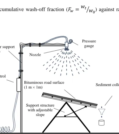
Data used in this study were collected from a series of laboratory experiments carried out using 14
an artificial rainfall generator, a 1 m2 bituminous road surface and a continuous wash-off 15
measuring system (Fig.1). This data contain sediment wash-off data measured against different 16
combinations of rainfall intensity, catchment surface slope and initial sediment load. The road 17
surface was prepared using bituminous asphalt concrete and had a mean texture depth index of 18
0.4 mm. D10, D50 and D90 of the sand used in the experiment are 300 m,450 m and 600 m 19
respectively. Five intensities ranging from 33-155 mm/hr, four slopes ranging from 2-16 % and 20
three initial loads ranging from 50 - 200 g/m2 were tested in these experiments. For more details 21
on the experimental setup, selection of experimental conditions and data collection the readers 22
6
are referred to Muthusamy et al. (2018). As reported in Muthusamy et al. (2018) the effect of 1
initial load on wash-off process was found to be negligible. Hence in this study, experimental 2
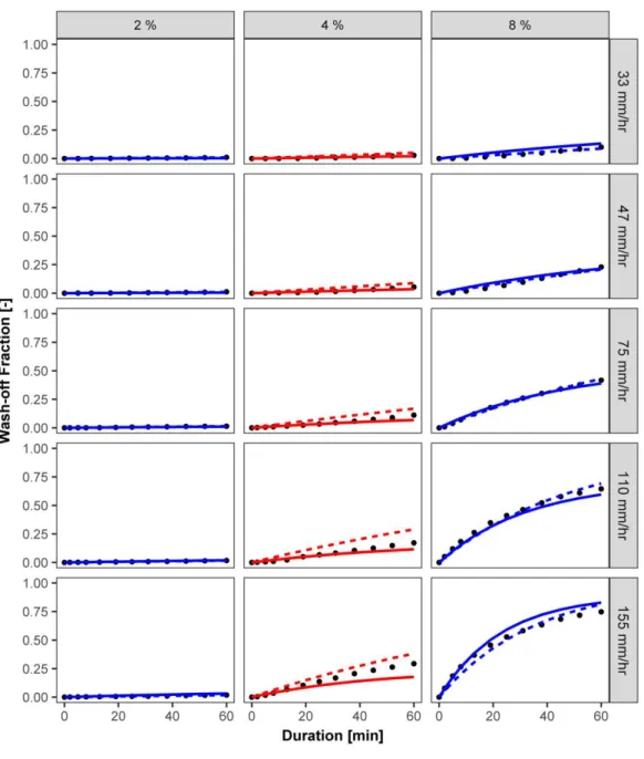
results from a constant initial load of 200 g/m2 as presented in Fig. 2 were used. This figure 3
shows the variation of cumulative wash-off fraction ( ) against rainfall intensity 4
and surface slope. 5
6
Figure 1. Sketch of the experimental setup
7
Note that the 16% slope was eliminated from the data, given that such slopes on road surfaces 8
are extreme scenarios and exist only in rare locations. For example, the Department of 9
Transport in the UK suggests a maximum gradient of 10% for roads other than in exceptional 10
circumstances (Manual for Streets, 2009). Since one of the aims of the study is to develop a 11
single model with a fixed set of parameters, the inclusion of results from such an extreme 12
scenario in the calibration may affect the performance of the model for more general cases. 13
Nozzle
Pressure gauge
Bituminous road surface (1 m × 1m)
Rainfall simulator support structure
Support structure with adjustable
slope
Sediment collection Rainfall simulator control
7 1
Figure 2: Selected results from Muthusamy et al. (2018): Variation of wash-off fraction for different
2
combinations of rainfall intensity and surface slope
3
2.2 The modified wash-off model structure and its rationale
4
The main objective is to replace the calibration parameters in Eq. 2 with functions of surface 5
slope and rainfall intensity, consequently adding a more physically realistic structure to the 6
model. This should make the model robust to new combinations of rainfall intensity and surface 7
slope. To do so, the properties of the model that are sensitive to such parameters need to be 8
identified and understood. From Eq. 2 there are two parameters which define the characteristics 9
of a wash-off curve. The first parameter, , defines the highest wash-off fraction for a given 10
combination of rainfall intensity and a slope. The second, k, defines how fast the wash-off 11
curve reaches the maximum fraction for a given surface slope and rainfall intensity, and hence 12
8
reflects the erosion rate from the catchment surface. Hence, and k were proposed to be 1
replaced with functions of surface slope and rainfall intensity, as shown in Eq. 3 and Eq. 4. 2
3
4
Where are constants1, is the representative rainfall intensity of a rainfall event (e.g. 5
in this case the constant rainfall intensity set during the experiment, please refer to section 3.4 6
for discussion on the use of representative rainfall intensities), is the catchment surface slope. 7
The following criteria were considered when defining Eq. 3 and Eq. 4, while also trying to keep 8
these functions as simple as possible to reduce the number of constants: 9
– as explained before is a capacity factor which defines the maximum fraction 10
from the initially available sediment that can ever be washed off from a rainfall event 11
for a given slope. Hence, ranges from 0 to 1 and increases with both surface slope 12
and (representative) rainfall intensity of the event. When either of the representative 13
rainfall intensity or slope is zero is zero. 14
– defines the wash-off rate and it also increases with rainfall intensity and surface 15
slope. But it should be noted that in the exponential term is cumulative rainfall depth 16
at time t, i.e. which is already a function of average rainfall intensity over time t, . 17
Hence was taken as a (linear) function of slope only. The complete exponential term 18
reads as which is function of both rainfall intensity and surface slope. 19
Hereafter this new exponential model will be referred as NEM and the original exponential 20
model as shown in Eq. 1 will be referred as OEM. 21
1 Although are constant, in Bayesian inference they are referred to as model parameters to aid the readers
9
2.3 Estimation of model parameters and associated uncertainty
1
Bayesian inference was used to estimate the parameter probability distribution, which allows 2
prior knowledge on the parameters to be incorporated in the estimation and also formally 3
quantifies uncertainty in the estimation (Dotto et al., 2012; Freni and Mannina, 2010; Del 4
Giudice et al., 2013). In addition, it also helps to capture the dependence structure between 5
parameters (Dotto et al., 2012). Bayesian inference requires the definition of the likelihood 6
function and the prior distribution of the parameters. 7
2.3.1
The likelihood function
8
In addition to finding the best estimate of the parameters, we are also interested in the 9
uncertainty associated with the parameter estimation and consequently the uncertainty in the 10
prediction of the wash-off fraction. One way of doing this is to include the error terms which 11
represent the dominant sources of uncertainty explicitly in the likelihood function. We used 12
an error model which accounts for errors due to the model structural deficit (model bias, ) 13
and measurement noise ( ). is modelled as an autoregressive stationary random process 14
and modelled as an independent identically distributed (IID) normal noise. Hence, an 15
observed output, can be formulated as 16
17
Where x is the external drivers, is deterministic model parameters, error model parameters 18
and is deterministic model output. In this case, is observed wash-off fractions 19
(Fw) and is the deterministic model output predicted from NEM (fw ). x represents rainfall 20
intensity and surface slope. represents parameters . represents error model 21
parameters , and in which and are standard deviation and the correlation 22
length respectively that characterise the autoregressive stationary random process and, is 23
10
the standard deviation of the measurement noise. Given the error description of Eq. 5, we define 1
as a multivariate Gaussian distribution with covariance matrix and 2
as independent, identical normal noise. Therefore, the analytic formulation of the likelihood 3
function with n number of observation can be formulated as 4
det exp
5
6
The covariance matrix was formulated using covariance in time calculated using OU 7
process (Uhlenbeck and Ornstein, 1930). For hydrological applications, OU process assumed 8
to be a simple description of underlying mechanisms leading to a decay of correlation in time 9
(Del Giudice et al., 2013; Sikorska et al., 2012; Yang et al., 2007). A detailed description of 10
the formulation of covariance matric using OU process can be found in Del Giudice et al. 11
(2013). An autoregressive error model represents model structural deficit better than IID as it 12
accounts for the “memory” in the error time series (Del Giudice et al., 2013). This 13
autoregressive bias error model was originally suggested in other generic statistical 14
applications (Bayarri et al., 2007; Craig et al., 2001; Higdon et al., 2004; Kennedy and 15
O’Hagan, 2001) and later adapted for environmental engineering applications (Reichert and 16
Schuwirth, 2012). 17
2.3.2
Prior distribution of parameters and constraints
18
Since the introduced parameters are all new, there is no previous estimation of the 19
exact parameters, but a range for each parameters can be derived using our knowledge of the 20
wash-off process, observational data, and the prior belief about values of and . 21
11
Values of were derived from previous estimations of k as equals to k/s. The list of k values 1
derived from previous studies is given in Table. 1. From the table, the range of 0 – 10 were 2
selected for k. In the absence of any information on slope in most of these studies same range 3
for was used considering a minimum slope of 1%. Hence a uniform prior with the range 0-4
1000 was used as a prior distribution for .A uniform prior distribution of model parameters 5
can be used when there is not enough evidence available to choose a different type of 6
distribution (Dotto et al., 2012; Freni and Mannina, 2010) 7
Table 1: k values from the literature
8
Reference Land use/catchment type Value k (mm-1)
Alley (1981)
Nakamura (1984)
Huber and Dickinson (1992)
Millar (1999) Egodawatta et al. (2007) Urban catchment Various General Residential
Concrete and asphalt roads
0.036-0.43 0.05-10 0.04-0.4 0.21 5.6 ×10⁻⁴– 8.0 ×10⁻⁴ 9
As discussed previously, the range of is 0-1 because wash off fraction cannot be more than 10
1. This leads to the constraint .. The implication of this constraint in the 11
definition of prior probability is not straightforward as it involves three parameters, hence this 12
constraint was used during the estimation of likelihood probability. 13
It is challenging to define prior distributions for the error model parameters 14
especially in the case of wash-off modelling as examples from such applications in literature 15
are currently lacking. Out of the three parameters, some information on the measurement noise 16
12
represented by can be obtained by frequentist tests, i.e. repeating the experiments 1
sufficiently large number of times. But it is not always possible given the limitation in allocated 2
resources and time. In the absence of much information on any of the error parameters, a 3
uniform prior with the range from 0 to 1(= maximum wash-off fraction) was used for 4
both and a uniform prior with the range of 0 – 200 min was used for correlation 5
length. This range is selected as error correlation is expected to be insignificant beyond such 6
time length. 7
2.3.3
Bayesian inference
8
Once the prior distributions (the probability of deterministic and error model 9
parameter, and without considering the observed output, ), and the likelihood 10
function (the probability of seeing the observed output, , as generated by a model with 11
deterministic and error model parameter, and ), are defined, the posterior 12
distribution of the deterministic and error model parameters (the conditional probability of 13
and once the observed output, has been taken into account) can be formulated as, 14
15
Since the direct analytical calculation of is generally not possible, numerical 16
techniques such as Markov Chain Monte Carlo (MCMC) simulations have to be applied to 17
generate samples for this distribution. MCMC techniques generate a random walk through the 18
parameter space which will converge to the posterior distribution. In this study, we used robust 19
adaptive Metropolis MCMC sampler presented in Vihola (2012) which is implemented in an 20
R package, adaptMCMC (Scheidegger, 2017).
13
2.4 Performance assessment
1
Experimental data with 2% and 8% slopes (two-thirds of the total data) were used for 2
calibration of NEM and the data from the 4% slope (one-third of the total data) were used for 3
verification. The optimal value of each parameter c1…c4 obtained during the calibration stage 4
was then used for validation. Furthermore, the performance of NEM was compared against 5
OEM during both calibration and validation stages. In the case of NEM, the k value was 6
calibrated for each and every combination of surface slope and rainfall intensity during the 7
calibration stage. Linear interpolation of these calibrated k values was then used to obtain new 8
k values during the validation stage for a new surface slope condition. 9
In addition to deterministic prediction, prediction uncertainty of NEM was also obtained during 10
both calibration and validation stages. Parameter and total predictive uncertainty (parameter 11
uncertainty + model bias + measurement noise) were predicted by sampling from posterior 12
multivariate distributions of parameters c1,..c4. Parameter uncertainty was estimated by using 13
deterministic model ( x ) runs and predictive uncertainty was estimated by using the 14
deterministic model together with error model components. 15
16
3. Results and discussion
17
3.1 Model performance
18
Figure 3 shows the model output with the optimal values for (Table. 1) with maximum 19
posterior probability density, i.e. the most probable values given the prior and observed data. . 20
It can be seen from Fig. 3 that with calibration data, NEM with fixed values of parameters 21
, corresponding to the maximum posterior probability density, performs as well as the 22
OEM which was calibrated for each and every combination of surface slope and rainfall 23
14
intensity separately. From Table 2, it can be seen that the difference in sum of root mean square 1
error (RMSEOEM - RMSENEM) from the ten calibrated set of data is -0.07 (Wash-off fraction). 2
However, the robustness of NEM over OEM can be seen during the verification stage where 3
the NEM performs better than the OEM in several cases. The difference in sum of root mean 4
square error (RMSEOEM - RMSENEM) from 5 sets of data during verification stage is 0.09 5
(Wash-off fraction). The drawback with OEM is that for a set of new catchment conditions 6
where OEM has not been calibrated before k value needs to be calculated using 7
interpolation/extrapolation. This might lead to the underperformance of OEM during validation 8
stage as shown in the Fig. 3. Considering the overall performance, the NEM with only 4 9
parameters ) performs better than OEM with 15 parameters (k1,…,k15). Hence, the 10
NEM does not only avoid the need of interpolation to predict the calibration parameter values, 11
it also performs as well as the calibrated OEM. 12
Table 1: Optimal values of constants of Eq. 3 and Eq. 4
13
c1 c2 c3 c4
3.99 0.672 1.99 0.208
14
Table 2: Performance of OEM and NEM
15
Model
Sum of root mean square error (RMSE)
Calibration Verification
OEM 0.11 0.20
15 1
Figure 3: Comparison of the model performance
2
3.2 Parameter distribution and correlation
3
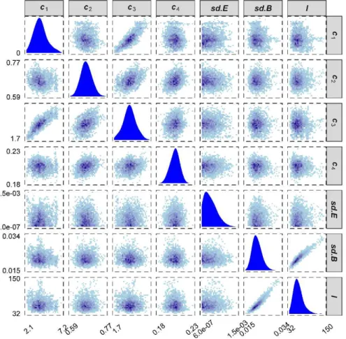
This section discusses the posterior distribution of parameters and their multivariate behaviour. 4
Figure 4 shows posterior distributions and a bivariate matrix of the deterministic and error 5
model parameters. The most likely value of and are 0.02 (2%) and 0.002 (0.2%) 6
16
respectively, showing that most of the uncertainty in the wash-off estimation can be explained 1
by the model bias and that uncertainty due to measurement noise is negligible. Although these 2
are approximate representations of the actual system and corresponding uncertainty, we believe 3
that the experiments were conducted with as high a quality as possible. This is one of the reason 4
why a road surface as small as 1 sq.m was selected as it gives a better control over the 5
experimental set-up. For example the smaller surface area keeps the spatial variability of the 6
rainfall to the minimum. Furthermore, it also keeps the sediment loss during the experiment to 7
insignificant. The maximum sediment loss observed during an experiment was less than 2% 8
which is an indication of the good quality control. 9
Looking at the bivariate plots, there is a strong positive correlation between parameters and 10
which indicates that these two parameters compensate each other in order to maximise the 11
posterior probability. This can also be seen between parameters and , but to a lesser extent. 12
Similarly, the strong positive correlation between and means that these parameters 13
compensate each other in order to fit the autoregressive error model .Bayesian inference 14
helps resolve such identifiability issues by allowing for informative priors. Therefore, for real 15
cases, where we have reasons to believe that one of the two parameters should be more 16
constrained, the other parameter value will automatically come out to be constrained after joint 17
inference. 18
17 1
Figure 4: Parameter distribution and bivariate correlation
2
3.3 Estimation of parameter and predictive uncertainty
3
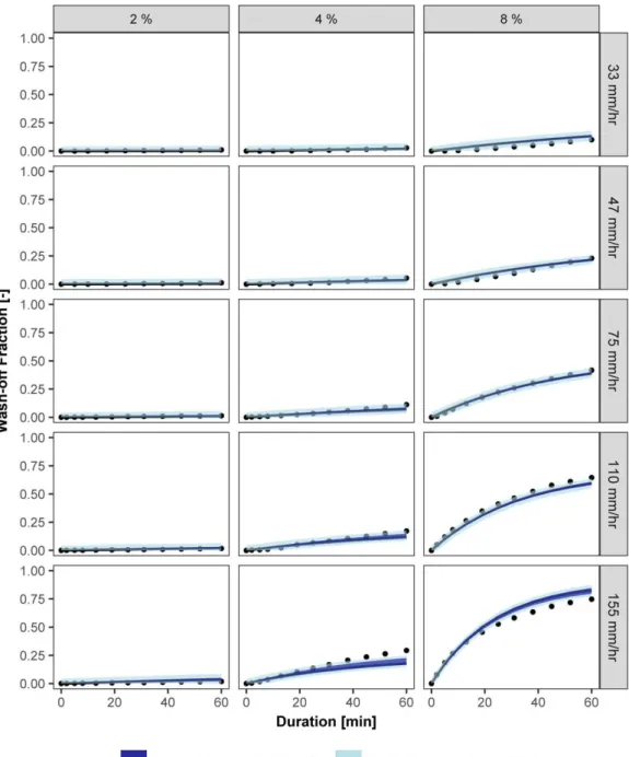
Figure 5 shows the uncertainty associated with the estimation of the wash-off fraction. 4
Parameter uncertainty was estimated by using deterministic model ( x ) runs and 5
predictive uncertainty was estimated by using the deterministic model together with error 6
model components. Since the latter also includes the uncertainty due to model bias and 7
measurement noise these bands are wider than the parameter uncertainty. The total predictive 8
uncertainty which accounts for parameter uncertainty, model bias and measurement noise 9
accounts for ~ 0.1 (10%) uncertainty in the wash-off fraction. This constant trend of predictive 10
uncertainty is a reflection of the fact that the error model used here is not explicitly input-11
18
dependent bias model, but rather it is a constant bias (variance) model. On the other hand, 1
parameter uncertainty increases with increasing wash-off fraction as the variance of parameter 2
uncertainty proportionally increases with mean prediction. The parameter uncertainty accounts 3
for a maximum of 0.06 (6%) wash-off fraction when 95% predictive interval is considered. 4
5
Figure 5: Uncertainty associated with the estimation of wash-off fraction using NEI
19
To check the reliability of the uncertainty estimation, prediction interval coverage probability 1
(PICP, Ref Eq.8) which measures the probability that the observed values lie within the 2
estimated prediction intervals (Shrestha and Solomatine, 2006) was used. 3
4
Where, are upper and lower boundary of the considered prediction interval at time t 5
for a given slope and rainfall intensity, is corresponding measured wash-off fraction at time 6
t. For a better performance, PICP should be close to the considered prediction interval, which 7
is 95% in this case. The calculated PICP during validation stage is 82%, so the corresponding 8
accuracy of the uncertainty estimation is around ~ 85% which essentially means that the error 9
model is able to predict the uncertainty reasonably well. 10
3.4 General discussion
11
IID is the most commonly used form of error model in urban hydrology (Breinholt et al., 2012; 12
Dotto et al., 2011; Freni et al., 2009; Sage et al., 2015) mainly because of its simplicity. 13
However, it requires the absence of a serial correlation in the error distribution, which can lead 14
to underestimation of uncertainty and biased parameter estimates (Del Giudice et al., 2013). 15
Error process of hydrological phenomena, such as sediment wash-off, are shown to be 16
temporally auto-correlated and assumption of independence is not satisfied (Schoups and 17
Vrugt, 2010; Sage et al., 2016). likelihood function based on uncorrelated error model generally 18
leads to narrower posterior probability densities, which results in overconfident parameter 19
estimates and unreliable uncertainty intervals. An autoregressive model helps in preventing 20
such biases both during inference and prediction. Unlike IID, where each data point is a sample 21
of the error distribution, an autoregressive process takes the whole time series of errors as one 22
20
sample realization of the process, (in an n-dimensional space), therefore avoiding 1
overconfidence in parameter estimation. For example, Sage et al. (2015) acknowledged that 2
their assumption to model error process associated with wash-off modelling as IID was found 3
to be invalid. Further, Sage et al., (2016) showed that the use of IID to represent the structural 4
deficit of sediment wash-off models violates the statistical properties of the structural deficit 5
and it may result in unreliable estimation of model parameters and total predictive uncertainty. 6
An autoregressive model accounts for this autocorrelation of the error and hence, it represents 7
the structural deficit better. 8
This error model can be further improved by accounting for non-normality of the structural 9
bias. However, this adds more complexity and such added complexity could be an acceptable 10
compromise when there is a very large number of data points to learn about the error model 11
parameters. In our case, the current description of errors seems adequate as suggested by 12
verification measures that show around 85% accuracy of the error models in capturing the 13
uncertainty. Further, we assumed a constant bias to keep this autoregressive error model 14
simple. Nevertheless, it is also possible to describe it as an input – dependent bias (Del Giudice 15
et al., 2013) where bias can be a function of both slope and intensity. The advantage of such 16
bias description still needs to be investigated in the uncertainty analysis of wash-off modelling. 17
Note that in addition to rainfall intensity and surface slope, other parameters such as sediment 18
size and surface texture will also affect the sediment wash-off, but due to the limitations in the 19
data used in this study, the NEM does not include the effect of these parameters. With smaller 20
sediment sizes and smoother surfaces, the wash-off is expected to be higher. For example, 21
Egodawatta et al. (2007) in a similar experimental study used a larger range (0 – 1000 µm) 22
sediment resulting in a relatively higher wash-off fraction. Further, Hong et al., (2016) in their 23
studies used a sediment range of 0- 400 µm and showed that most (> 90%) of the finest particles 24
21
are removed at the beginning of a rainfall event, with about 10%–20% of medium-size particles 1
are removed over the later part of the even. These studies show that selection of sediment size 2
affects the sediment wash-off process significantly. Hence, the application of the NEM needs 3
to be checked against different sediment sizes and also against different surface textures. It is 4
expected that the values of c1,..,c4 will be different for different particle size distribution of the 5
road sediment and/or different surface roughness. The inclusion of the effect of these 6
parameters explicitly might introduce more complexity in the equation, nevertheless, such an 7
equation can be applied globally regardless of individual catchment conditions. This is one of 8
the research areas in sediment wash-off modelling that requires to be investigated in detail. 9
While experimental set-ups like the one used in this study give great flexibility to replicate the 10
real hydrological processes such as sediment wash-off, there are still some limitations which 11
need to be taken into account. The exponential wash-off model was improved based on 12
experimental results which were obtained from rainfall events with constant rainfall intensity 13
throughout the duration of an event. Keeping the rainfall intensity constant makes it easier to 14
understand the physical wash-off process and to consequently modify the wash-off model. In 15
fact, most of the previous studies used a constant intensity rainfall event to understand the 16
wash-off process and consequently apply the results to develop and improve the wash-off 17
equations. These studies include Sartor and Boyd (1972) where the exponential model was 18
originally proposed and Egodawatta et al. (2007) where the capacity factor was first introduced 19
in the exponential wash-off. However, constant intensity rainfall events are never the case in 20
reality. Nevertheless, equation proposed by Sartor and Boyd (1972) and consequent refined 21
version (e.g. Egodawatta et al., 2007) were all shown to be applicable for real case studies too. 22
For example, Brodie and Egodawatta (2011) on a follow-up study on Egodawatta et al. (2007) 23
showed that the use of mean rainfall intensity of real a rainfall event as a representative intensity 24
22
to derive produced reliable predictions. In this regard, application of NEM also needs to be 1
checked against wash-off events resulted from real rainfall events. Such validation also needs 2
information about surface slope. 3
It can also be noted that the rainfall intensities used in this experiments are generally high 4
compared to rainfall intensities observed in the real world. However, the minimum intensity of 5
~ 30 mm/hr was chosen based on the trial experiments to produce measurable sediment wash-6
off amounts from the surface. For example, at 2% slope, even the rainfall intensity of 155 7
mm/hr produced only 6g wash-off total wash-off at the end of 60 min. In addition to selected 8
sediment size and surface roughness, surface size also a deciding factor in the amount of 9
washed off sediment as the larger surface will have a proportionally higher initial sediment 10
load. On the other hand, unlike sediment size and surface roughness, surface size does not 11
affect the underlying physical process and as a result, the wash-off fraction (= washed off 12
load/initial load) will remain same. This provides the flexibility in choosing the surface size 13
for similar wash-off experiments. The small surface size such as the one used in this study (1 14
× 1 m2) provides a degree of flexibility to change the experiment conditions (e.g. surface slope, 15
initial load) and makes it possible to run such a large number of experiments. Also, it helps to 16
keep the rainfall intensity fairly uniform over the surface. Similar sized experimental surfaces 17
have been used in recent studies to take advantage of the above-mentioned points (Egodawatta 18
et al., 2007; Al Ali et al., 2017). However, the trade-off is the physically lesser amount of 19
washed off sediment from the surface and consequently the limitation in testing very mild 20
rainfall conditions in these experiments. Hence, an optimal surface size needs to be chosen in 21
future studies which take into account the flexibilities in the experimental setup and the 22
minimum rainfall intensity that can produce a physically measurable sediment wash-off with 23
limited measurement error. However, rainfall intensities used in these experiments are 24
23
comparable to rainfall intensities used in similar previous wash-off studies. For example, 1
Egodawatta et al., (2007) used a rainfall intensity range of 40 mm/hr - 133 mm/hr and 20 mm/hr 2
- 133 mm/hr in their experiments to study the wash-off behaviour. Recently Al Ali et al., (2017) 3
used a constant rainfall intensity of 120 mm/hr in similar experimental settings to study the 4
wash-off behaviour from different surfaces. Due to the practical difficulty in covering a large 5
range of rainfall intensity in an experimental set-up, extrapolation of the equation/model 6
outside the experimental conditions is often used. Even the most widely used exponential 7
model was originally developed for much narrower intensity range of 8 mm/hr – 20 mm/hr 8
(Sartor and Boyd, 1972) and has been used widely for rainfall intensities that are well outside 9
this range. One of the reasons why this is an accepted practice could be that the pattern of 10
observations from previous studies indicate that the underlying physical transport process of 11
wash-off are quite similar, even outside the experimental conditions that are tested. For 12
instance, the inclusion of capacity factor as a function of rainfall intensity and slope would be 13
valid for smaller rainfall intensities as even higher intensities have a maximum capacity in 14
wash-off load as seen from the experimental results. Hence, although NEM has not been 15
calibrated against smaller rainfall intensities, we believe the model structure of NEM would 16
still be applicable to smaller rainfall intensities. Nevertheless, this should be verified in future 17
studies.
18
4. Conclusions
19
In this study, we proposed an improved exponential wash-off model where a more physically 20
realistic structure was added to the original exponential model by replacing the calibration 21
parameters with functions of external drivers associated with catchment surface and rainfall 22
characteristics. This improvement avoids the need for empirical look-up table/charts and 23
interpolation/extrapolation and introduces some transparency in the parameter estimation 24
24
which is otherwise a “black box” approach. Further, replacing the invariant calibration 1
parameters with functions of external drivers (i.e. rainfall intensity and surface slope) makes it 2
easier to investigate the propagation of errors in the external drivers (e.g. rainfall intensity) as 3
these external drivers are now explicitly defined in the new equation. This new exponential 4
model (NEM) was calibrated and verified using the experimental data collected for different 5
combinations of surface slopes and rainfall intensities. Bayesian inference, which allows the 6
incorporation of prior knowledge, was implemented to estimate the distribution of the 7
parameters of the newly introduced functions. In addition, by statistically describing model 8
bias and measurement noise, different sources of uncertainty in the prediction of NEM were 9
separately estimated. 10
During calibration, NEM with a fixed set of parameter values performs as well as OEM which 11
is calibrated for each and every experimental condition separately. At validation, NEM’s 12
performance improves over OEM, reflecting the ability of NEM to perform better under new 13
catchment conditions. Verification measures show the uncertainty estimates associated with 14
NEM predictions are plausible, indicating that the use of two error terms, autoregressive error 15
and independently identically distributed error, to represent model bias and measurement noise 16
respectively was a reasonable representation of the error process associated with sediment 17
wash-off modelling. The total predictive uncertainty which accounts for both model bias and 18
measurement noise accounts for ~ 0.1 (10%) uncertainty in wash-off fraction when 95% 19
predictive interval is considered out of which a maximum of 0.06 (6%) comes from the 20
parameter uncertainty. 21
It should be noted that the optimal values of c1,..,c4 in NEM needs to be checked against 22
different sediment sizes and different surface roughness as these are two other major external 23
drivers which would affect the sediment wash-off. Nevertheless, the model structure of NEM 24
25
would be applicable for any sediment size and surface texture as the underlying physical 1
processes will be the same as those on which the model structure of NEM was developed. 2
Acknowledgement
3
The authors thank Jörg Rieckermann for his engagement in profitable discussions. This 4
research was done as part of the Marie Curie ITN - Quantifying Uncertainty in Integrated 5
Catchment Studies project (QUICS). This project has received funding from the European 6
Union’s Seventh Framework Programme for research, technological development and
7
demonstration under Grant Agreement no. 607000. 8
Reference
9
Akan, A. O.: Pollutant Washoff by Overland Flow, J. Environ. Eng., 113(4), 811–823, 10
doi:10.1061/(ASCE)0733-9372(1987)113:4(811), 1987. 11
Al Ali, S., Bonhomme, C., Dubois, P. and Chebbo, G.: Investigation of the wash-off process 12
using an innovative portable rainfall simulator allowing continuous monitoring of flow and 13
turbidity at the urban surface outlet, Sci. Total Environ., 609, 17–26, 14
doi:10.1016/j.scitotenv.2017.07.106, 2017. 15
Alley, W. M.: Estimation of Impervious-Area Washoff Parameters, Water Resour. Res., 17(4), 16
1161–1166, 1981. 17
Bayarri, M. J., Berger, J. O., Paulo, R., Sacks, J., Cafeo, J. A., Cavendish, J., Lin, C.-H. and 18
Tu, J.: A Framework for Validation of Computer Models, Technometrics, 49(2), 138–154, 19
doi:10.1198/004017007000000092, 2007. 20
Breinholt, A., Møller, J. K., Madsen, H. and Mikkelsen, P. S.: A formal statistical approach to 21
representing uncertainty in rainfall–runoff modelling with focus on residual analysis and 22
26
probabilistic output evaluation – Distinguishing simulation and prediction, J. Hydrol., 1
472(Supplement C), 36–52, doi:https://doi.org/10.1016/j.jhydrol.2012.09.014, 2012. 2
Brodie, I. M. and Egodawatta, P.: Relationships between rainfall intensity, duration and 3
suspended particle washoff from an urban road surface, Hydrol. Res., 42(4), 239 LP-249 4
[online] Available from: http://hr.iwaponline.com/content/42/4/239.abstract, 2011. 5
Coleman, T. J.: A comparison of the modelling of suspended solids using SWMM3 quality 6
prediction algorithms with a model based on sediment transport theory., in 6th Int. Conf. on 7
Urban Storm Drainage, ASCE, Reston, VA., 1993. 8
Collins, P. G. and Ridgeway, J. W.: Urban storm runoff quality in southeast Michigan, J. 9
Environ. Eng. Div., 106(EEl), 153–162, 1980. 10
Craig, P. S., Goldstein, M., Rougier, J. C. and Seheult, A. H.: Bayesian Forecasting for 11
Complex Systems Using Computer Simulators, J. Am. Stat. Assoc., 96(454), 717–729 [online] 12
Available from: http://www.jstor.org/stable/2670309, 2001. 13
Deletic, A., Maksimovic, C. and Ivetic, M.: Modelling of storm wash-off of suspended solids 14
from impervious surfaces, J. Hydraul. Res., 35(1), 99–118, doi:10.1080/00221689709498646, 15
1997. 16
Dotto, C. B. S., Kleidorfer, M., Deletic, A., Rauch, W., McCarthy, D. T. and Fletcher, T. D.: 17
Performance and sensitivity analysis of stormwater models using a Bayesian approach and 18
long-term high resolution data, Environ. Model. Softw., 26(10), 1225–1239, 19
doi:https://doi.org/10.1016/j.envsoft.2011.03.013, 2011. 20
Dotto, C. B. S., Mannina, G., Kleidorfer, M., Vezzaro, L., Henrichs, M., McCarthy, D. T., 21
Freni, G., Rauch, W. and Deletic, A.: Comparison of different uncertainty techniques in urban 22
stormwater quantity and quality modelling, Water Res., 46(8), 2545–2558, 23
27 doi:10.1016/j.watres.2012.02.009, 2012.
1
Egodawatta, P. and Goonetilleke, A.: Understanding road surface pollutant wash-off and 2
underlying physical processes using simulated rainfall, Water Sci. Technol., 57(8), 1241–1246, 3
doi:10.2166/wst.2008.260, 2008. 4
Egodawatta, P., Thomas, E. and Goonetilleke, A.: Mathematical interpretation of pollutant 5
wash-off from urban road surfaces using simulated rainfall, Water Res., 41(13), 3025–3031, 6
doi:10.1016/j.watres.2007.03.037, 2007. 7
Freni, G. and Mannina, G.: Bayesian approach for uncertainty quantification in water quality 8
modelling: The influence of prior distribution, J. Hydrol., 392(1), 31–39, 9
doi:https://doi.org/10.1016/j.jhydrol.2010.07.043, 2010. 10
Freni, G., Mannina, G. and Viviani, G.: Uncertainty assessment of an integrated urban drainage 11
model, J. Hydrol., 373(3), 392–404, doi:https://doi.org/10.1016/j.jhydrol.2009.04.037, 2009. 12
Del Giudice, D., Honti, M., Scheidegger, A., Albert, C., Reichert, P. and Rieckermann, J.: 13
Improving uncertainty estimation in urban hydrological modeling by statistically describing 14
bias, Hydrol. Earth Syst. Sci., 17(10), 4209–4225, doi:10.5194/hess-17-4209-2013, 2013. 15
Guy, H. P.: Sediment Problems in Urban Areas, Geol. Surv. Circ. 601-E, U.S. Geol. Surv., 16
1970. 17
Higdon, D., Kennedy, M., Cavendish, J., Cafeo, J. and Ryne, R.: Combining Field Data and 18
Computer Simulations for Calibration and Prediction, SIAM J. Sci. Comput., 26(2), 448–466, 19
doi:10.1137/S1064827503426693, 2004. 20
Hong, Y., Bonhomme, C., Le, M. H. and Chebbo, G.: New insights into the urban washoff 21
process with detailed physical modelling, Sci. Total Environ., 573, 924–936, 22
28 doi:10.1016/j.scitotenv.2016.08.193, 2016. 1
Huber, W. C. and Dickinson, R. E.: Storm Water Management Model , Version 4 : User’s
2
Manual, Athens, Ga., 1992. 3
Kennedy, M. C. and O’Hagan, A.: Bayesian calibration of computer models, J. R. Stat. Soc.
4
Ser. B (Statistical Methodol., 63(3), 425–464, doi:10.1111/1467-9868.00294, 2001. 5
Lawler, D. M., Petts, G. E., Foster, I. D. L. and Harper, S.: Turbidity dynamics during spring 6
storm events in an urban headwater river system: The Upper Tame, West Midlands, UK, Sci. 7
Total Environ., 360(1–3), 109–126, doi:10.1016/j.scitotenv.2005.08.032, 2006. 8
Millar, R. G.: Analytical determination of pollutant wash-off parameters, J. Environ. Eng., Vol. 9
125,(No. 10 (Technical Note)), 989–992, 1999. 10
Mitchell, G., Lockyer, J. and McDonald, A. .: Pollution Hazard from Urban Nonpoint Sources: 11
A GIS-model to Support Strategic Environmental Planning in the UK, Tech. Report, Sch. 12
Geogr. Univ. Leeds, 1,2, 240pp, 2001. 13
Muthusamy, M., Tait, S., Schellart, A., Beg, M. N. A., Carvalho, R. F. and de Lima, J. L. M. 14
P.: Improving understanding of the underlying physical process of sediment wash-off from 15
urban road surfaces, J. Hydrol., 557, 426–433, 16
doi:https://doi.org/10.1016/j.jhydrol.2017.11.047, 2018. 17
Nakamura, E.: Factors affecting stormwater quality decay coefficient, in Proceedings of the 18
Third International Conference on Urban Storm Drainage, edited by A. S. P. Balmer, P. 19
Malmquist, pp. 979 – 988, Goteborg, Sweden., 1984. 20
Reichert, P. and Schuwirth, N.: Linking statistical bias description to multiobjective model 21
calibration, Water Resour. Res., 48(9), doi:10.1029/2011WR011391, 2012. 22
29
Sage, J., Bonhomme, C., Al Ali, S. and Gromaire, M. C.: Performance assessment of a 1
commonly used “accumulation and wash-off” model from long-term continuous road runoff 2
turbidity measurements, Water Res., 78, 47–59, doi:10.1016/j.watres.2015.03.030, 2015. 3
Sage, J., Bonhomme, C., Berthier, E. and Gromaire, M.-C.: Assessing the Effect of 4
Uncertainties in Pollutant Wash-Off Dynamics in Stormwater Source-Control Systems 5
Modeling: Consequences of Using an Inappropriate Error Model, J. Environ. Eng., 6
143(August), 1–9, doi:10.1061/(ASCE)EE.1943-7870.0001163, 2016. 7
Sartor, J. D. and Boyd, B. G.: Water pollution aspects of street surface contaminants., , EPA 8
Rep. 11024 DOC 07-71, (NTIS PB-203289), 1972. 9
Scheidegger, A.: adaptMCMC: Implementation of a Generic Adaptive Monte Carlo Markov 10
Chain Sampler, [online] Available from: http://cran.r-project.org/package=adaptMCMC, 11
2017. 12
Schoups, G. and Vrugt, J. A.: A formal likelihood function for parameter and predictive 13
inference of hydrologic models with correlated, heteroscedastic, and non-Gaussian errors, 14
Water Resour. Res., 46(10), 1–17, doi:10.1029/2009WR008933, 2010. 15
Shaw, S. B., Stedinger, J. R. and Walter, M. T.: Evaluating Urban Pollutant Buildup/Wash-Off 16
Models Using a Madison, Wisconsin Catchment, J. Environ. Eng., 136(February), 194–203, 17
doi:10.1061/(ASCE)EE.1943-7870.0000142, 2010. 18
Shrestha, D. L. and Solomatine, D. P.: Machine learning approaches for estimation of 19
prediction interval for the model output., Neural Netw., 19(2), 225–35, 20
doi:10.1016/j.neunet.2006.01.012, 2006. 21
Sikorska, A. E., Scheidegger, A., Banasik, K. and Rieckermann, J.: Bayesian uncertainty 22
assessment of flood predictions in ungauged urban basins for conceptual rainfall-runoff 23
30
models, Hydrol. Earth Syst. Sci., 16(4), 1221–1236, doi:10.5194/hess-16-1221-2012, 2012. 1
Uhlenbeck, G. E. and Ornstein, L. S.: On the theory of the Brownian motion, Phys. Rev., 36(5), 2
823–841, doi:10.1103/PhysRev.36.823, 1930. 3
Vihola, M.: Robust adaptive Metropolis algorithm with coerced acceptance rate, Stat. Comput., 4
22(5), 997–1008, doi:10.1007/s11222-011-9269-5, 2012. 5
Yang, J., Reichert, P. and Abbaspour, K. C.: Bayesian uncertainty analysis in distributed 6
hydrologic modeling: A case study in the Thur River basin (Switzerland), Water Resour. Res., 7
43(10), n/a-n/a, doi:10.1029/2006WR005497, 2007. 8
Zug, M., Phan, L., Bellefleur, D. and Scrivener, O.: Pollution wash-off modelling on 9
impervious surfaces: Calibration, validation, transposition, in Water Science and Technology, 10
vol. 39, pp. 17–24, No longer published by Elsevier., 1999. 11 12 13 14 15 16 17 18 19 20 21 22 23