Flood Damage Model Case Study Results

(1)

Work Package:

WP3 Impact Assessment

Document Name:

Flood Damage Model Case Study Results

Date:

11 August 2014

Report Number:

D3.4

Revision Number:

2 Deliverable Number:

D3.4

Due date for deliverable:

31 December 2011

Actual submission date:

15 August 2014

Author:

University of Exeter

*************************

CORFU is co-funded by the European Community Seventh Framework Programme.

CORFU is a Collaborative Project in the FP7 Environment Programme Start date April 2010, duration 4 Years.

******************************

Document Dissemination: PU (Publically disseminated)

Co-ordinator: University of Exeter, United Kingdom Project Contract No: 244047

Project website: www.corfu7.eu

ACKNOWLEDGEMENTS

The work described in this publication was supported by the European Community’s Seventh Framework Programme through the grant to the budget of CORFU Collaborative Research on Flood Resilience in Urban Areas, Contract 244047.

DISCLAIMER

This document reflects only the authors’ views and not those of the European Community. The work may rely on data from sources external to the CORFU consortium. Members of the Consortium do not accept liability for loss or damage suffered by any third party as a result of errors or inaccuracies in such data. The information in this document is provided “as is” and no guarantee or warranty is given that the information is fit for any particular purpose. The user thereof uses the information at its sole risk and neither the European Commission nor any member of the CORFU Consortium is liable for any use that may be made of the information. ©CORFU Consortium

(2)

2

DOCUMENT INFORMATION:

Title

Flood Damage Model Case Study Results

Lead Authors

Michael Hammond, Albert Chen, Slobodan Djordjevic

Contributors

David Butler, Marc Velasco, Beniamino Russo, David Khan, Jelena

Batica, Kapil Gupta, Yuwen Zhou, Natasa Manojlovic, Ming-Hsi Hsu

Distribution

PU - Public

Document

Reference

WP3/D3.4

DOCUMENT HISTORY:

Date Revision Prepared by Organisation Approved by Notes

01 July 2012

1 MJH UoE SDj

(3)

3

SUMMARY

This deliverable presents the flood damage model case study results for the current / baseline situation. The flood damage model developed and described in D3.3 is used to estimate the expected annual damage (EAD) using a range of simulated flood events in the case study cities. The differences in geographical, climate, cultural and socio-economic conditions will provide a wide range for model parameter settings. Historic data is used to calibrate and verify the extended flood damage assessment model. The influences of climate change and urban growth scenarios on flood damages for the case studies are examined to identify “hot-spots” that are vulnerable to flooding for given scenarios. The analysis of results will provide feedback to WP1 and WP2 for adjusting urban growth prediction and setting up flood resilience measures.

Related deliverables

This deliverable requires inputs from:

 Deliverable 2.4 – flood hazard modelling results for present situation  Deliverable 3.3 – framework for flood damage assessment

This deliverable provides inputs for:

(4)

4

1 Introduction

This report will present the results of the damage or impact assessments undertaken in each of the case study cities. These assessments reflect the current state or existing situation, and these results serve as a benchmark from which future scenarios and the corresponding flood impacts can be compared.

In this report, authors from each of the case study cities will describe the main steps followed in the flood damage assessment, using the flood damage model. This will include details of the hydraulic modelling, the driving conditions leading to flooding that have been simulated, the methodology of the damage assessment, and the main results, describing any particular damage hotspots. The authors will also comment on the key assumptions that have been made, and the limitations of the assessment. The report will be updated as more work is undertaken and the methodologies are developed further.

(8)

8

2 Case study Barcelona

2.1 Case study area overview

Barcelona with a population of 1,621,537 inhabitants within its administrative limits on a land area of 101.4 km2 (15,980 inhab./Km2) is located on the Northeast coast of Spain, facing the Mediterranean Sea, on a plateau limited by the mountain range of Collserola, the Llobregat river to the south-west and the Besòs river to the north east. The city benefits from a classic Mediterranean climate and occasionally suffers heavy rainfalls of great intensities generating flash flood events. The yearly average rainfall is 600 mm, but the maximum intensity in 5 min, corresponding to a return period of 10 years, is 204.7 mm/h. Consequently, it is not rare that 50 % of the annual precipitation occurs during two or three rainfall events. The morphology of Barcelona presents areas close to the Collserola Mountain with high gradients (with an average of 4%) and other flat areas near to the Mediterranean Sea with lower slopes (with an average of 1%) (Figure 2-1). There are 31 catchments in the city. This morphology produces flash floods in the bottom part of the city in case of heavy storm events.

Figure 2-1 Typical gradients and morphology in Barcelona. The red circle represents the location of Raval District.

A specific area of Barcelona, the Raval District, was selected as case study, considering, for the whole area, a flood risk assessment based on the hazard and vulnerability evaluation. The Raval District, with almost 50,000 inhabitants in an area of 1.09 km2 is one of the most densely populated areas in Europe (approx. 44,000 inh./km2). Figure 2-2 shows the boundaries of the Raval District and Barelona.

This district, located in a hollow area of the city, suffers from flooding problems when heavy storm events occur. These problems are caused by the excess of surface runoff and the poor capacity of the sewer system. Then, stormwater not conveyed into the sewer network and overflows from sewer manholes generate urban floods with low depths and high velocities. Moreover the hydrological response time of Raval District catchment is very short (less than 30 minutes). Such events produce significant hazard to the population, as well as economic damages to the buildings.

2.2 Scenarios

The impact assessment described in this deliverable is calculated for a single scenario: the present-day situation. Future deliverables will provide the impact assessment results that have been undertaken assuming different future scenarios (D3.8) and different measures and strategies (D3.9).

(9)

9

Figure 2-2. Case study area: the Raval district of Barcelona.

2.3 Hydraulic modelling

A detailed 1D/2D coupled model, simulating surface and sewer flows was developed using Infoworks ICM version 3.0 by Innovyze (2013). ICM solves the complete 2D Saint Venant equations in a finite volume semi-implicit scheme (Godunov, 1959) with a Riemann solver (Alcrudo and Mulet-Martí, 2005).

The estimation of flood depth in a very accurate way is crucial for a micro scale assessment as this one. Therefore, there was a need for a coupled 1D/2D approach in order to take into account surface flows coming from upstream catchments and the interactions between the two drainage layers (known, respectively, as ‘major system’ formed by streets, sidewalks, squares, etc. and ‘minor system’ formed by the sewer network), as shown in Figure 2-3.

Special attention was paid to the hydraulic characterization of the inlet systems (representing the interface between surface and underground flows) using experimental expressions achieved in the Technical University of Catalonia (Gómez and Russo, 2011).

In order to consider surface and sewer flows coming into the Raval District from upstream catchments, an extended area was considered in the study. Only main sewers were considered for these catchments, while main and secondary networks were taken into account for Raval District. The final model considered a total area of 44 km2 with 3874 nodes, 241 km of total pipe length and 6 major storage facilities with a total capacity of 170,000 m3.

A 2D mesh covered the whole analyzed domain with 403,822 triangles. Parks and other green areas were represented in the same 2D mesh, trough “2D infiltration zones” characterized by their specific hydrological, physical and geometric parameters, while buildings were represented as void areas.

(10)

10

Runoff produced in the building areas was estimated considering an approximation of single non-linear reservoir (whose routing coefficient depends on surface roughness, surface area, ground slope and catchment width) and directly conveyed into the sewer network. This goes in accordance with local practice in Barcelona, where roofs and terraces (approximately corresponding to 50% of the whole analyzed domain) are directly connected to the underground sewers.

Sewer model was calibrated and validated using data regarding 4 critical rainfall events occurred in 2011 and provided by CLABSA Control Center. These data concerned 11 rain gages, 29 limnimeters and several time series related to real time control devices. Moreover, other data collected in the post events emergency reports (elaborated by policemen and firemen), and amateur videos recorded during the selected storm events were used to calibrate surface flow. Detailed information about the features of the model and, above all, the interactions between 1D and 2D layers is available in other deliverables (D2.2 and D2.4) and Russo et al. (2012 and 2013).

Figure 2-3. Interaction of surface and sewer flow (dual drainage concept) (Schmitt et al. 2004)

2.4 Damage / impact modelling

The flooding problems that occur in the Raval produce significant hazard for traffic and pedestrians, as well as economic damages in terms of goods and properties. Since the goal of this study is to determine the cost-effectiveness of several adaptation strategies, an accurate economic appraisal of the damages is crucial. Then, comparing the baseline scenario with the future ones (taking into account both global changes and adaptation measures), the benefits of adaptation can be quantified and the different measures prioritized.

In the following sections, different types of impacts should be assessed. However, due to the area studied, only direct damages have been included. First of all, the direct tangible damages related to the buildings are assessed. Then, in an intangible way and giving several risk levels, the impacts to people and vehicles are calculated.

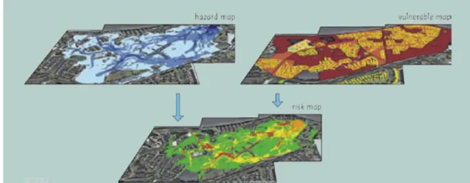
Risk is defined as the probability or threat of a hazard occurring in a vulnerable area and that may be avoided or minimised through preventive actions. For the three different impact categories, flood

(11)

11

risk is assessed in the same way. Flood risk maps related to each specific scenarios and return period are obtained by combining hazard maps and vulnerability maps, as shown in Figure 2-4.

Figure 2-4. Combination of hazard and vulnerability maps to produce a flood risk map.

In the case of direct tangible damages, risk is expressed in terms of monetary values thanks to the depths damage curves. For the other two categories, risk maps are created multiplying the vulnerability index (1, 2 or 3, corresponding to low, moderate and high vulnerability) by the hazard index (1, 2 or 3, corresponding to low, moderate and high hazard). Finally the total risk varies from 1 to 9 where higher levels indicate higher risk. This methodology is summarized in the following matrix (Figure 2-5).

Figure 2-5. Risk matrix obtained by multiplying the vulnerability index by the hazard index.

2.4.1 Direct tangible impacts

Regarding the scale of the study, Messner et al. (2007) proposed the following classification: macro, meso, and micro scales. Here, as the case study area is a city district of approximately 1 km2, the development of a micro-scale study is needed. Hence, as opposed to other scales, data requirements are high, and some properties must be considered on an individual basis.

As the flood damage assessment is an issue that has not been deeply studied in Spain, experiences from other countries (Penning Rowsell et al. 2005, Nascimiento et al. 2007, Kok et al. 2004, Reese et al. 2003) were reviewed. In general, the estimation of the damage caused by flooding focuses on the

1

2

3

1

2

3

2

4

6

3

6

9 Hazard

V

ul

ne

ra

bi

li

ty

Risk Matrix

(12)

12

flood depth. Therefore, depth-damage or stage-damage curves have been adopted in multiple locations around the world as the most commonly used technique to assess flood vulnerability. A vulnerability assessment of direct tangible damages at a micro-scale level will require the following three elements: stage-damage curves; flood depth maps; and land-use maps. In addition, in order to ease the calculation of the final vulnerability maps, the GIS-based toolbox developed in D3.3 will be used. Data regarding flood depths were already described in section 2.3. Following, the descriptions of depth damage curves and land-use maps used are presented.

2.4.1.1 Hazard levels for direct tangible impacts

Figure 2-6 shows the depths generated by the three rainfall events simulated. It is worth noting that, the model outputs (i.e. water depth in the streets) have been converted into water depth inside the buildings in order to ease the calculation of the damages. Consequently, Figure 2-6 shows water only inside the buildings and not in the streets. In addition, the reader should note that water depths of less than 15 cm will cause no damage, due to the depth damage curves developed. Therefore, although the light blue colour is sometimes widespread, only the values over 15 cm will be considered for the damage model.

For an event of 1 year return period, the flood problems are small and since most of them are small depths, they will not cause a lot of damages. For an event of 10 years of return period, there will be some localised problems on a rather small area of the district. When increasing the severity of the rain event, this area enlarges and the water depths also increase. Consequently, for a 100 year return period event, the model presents a generalised flood in the district, which is especially intense in the southern part. This situation can be explained considering that the drainage system of Barcelona is generally designed for a return period of 10 years.

Of course, the situation presented by the flood maps in Figure 2-6 is an upper bound of the actual situation. This is because both the synthetic rains used, and the assumption of having the same depth inside the buildings than in the streets leads to an overestimation of the depths. Nevertheless, since the final goal of this study is to compare the current situation to the future ones defined by the different scenarios that will be developed, using an upper bound will imply selecting the most robust strategies to cope with flood impacts.

(13)

13

Figure 2-6. Flood depths in the Raval district for a rain event of return period of 1 year (left), 10 years (center) and 100 years (right).

2.4.1.2 Vulnerability levels for direct tangible impacts

In this case, flood vulnerability is expressed as the combination of two different things: the stage-damage curves and the land-use maps. The two of them are explained in the following sections.

2.4.1.2.1 Stage-damage curves

Depending on the information available and the goals of the assessment, there are several types of depth-damage curves (Merz et al. 2010). As in Barcelona there is a lack of historical damage data, and the building typology may be remarkably different from other regions previously studied, following the recommendations of D3.3, it was decided to develop specific synthetic relative depth-damage curves for the city.

The curves are used to obtain damage costs for a certain water depth relative to the extent flooded. Then, multiplying the obtained value by the affected area of the building, the damage cost at a block scale is acquired.

These curves are calculated for different types of land-use. Taking into account the main uses identified in the case study area, six different categories have been defined (Figure 2-9). Then, via a what-if analysis and using flood expertise acquired from past flood events, a stage-damage curve for each type of building and economic activity has been obtained. These final stage-damage functions are composed by two independent curves. The first one, related to the re-conditioning of the building (cleaning, painting the walls, changing the floors or doors, etc.), has been obtained through the expertise gained in past local floods (with the collaboration of an expert in flooding damages appraisals for insurance companies). The second component is related to the damages to the contents, which have been developed using the FloReTo tool (Manojlovic & Pasche 2010). The several curves developed can be seen in Figure 2-7.

(14)

14

Figure 2-7. Depth damage curves for the buildings (left) and content (right) taking into account the local conditions of the Raval district.

The relationship between building and contents damages strongly depends on the type of land-use considered. Whereas in households the building damages tend to be higher than the contents’ (Thieken et al. 2005), this trend is not so clear in other land-uses. In the case of commercial use, flood losses are highly variable due to the differences depending on the kind of business considered (Gissing & Blong 2004). Since the Raval district mainly has small and simple retail shops with many goods, the curves define the content damages up to five times greater than the building ones. In order to assess the ability of the curves developed to represent the Raval case study, a survey was undertaken in the area. Taking advantage of the flood event that occurred on 31st July 2011, a series of interviews were carried out (Velasco & Cabello 2012). Although the number of affected people was small, the answers provided very interesting information which was very useful to validate the synthetic curves previously developed.

In addition, actual damage data from the Consorcio de Compensación de Seguros (CCS), the re-assurance that covers the catastrophic and extreme situations in Spain, were obtained for the same flood event in the Raval district. Altogether, a two-step validation was done: a qualitative one, using the general trends and behaviours extrapolated from the surveys; and a semi-quantitative one, comparing the flood damage maps and total figures for the studied area.

Some of the general outcomes of the surveys applied in the curves are: in the Raval district, damages to contents will be more important than the damages to the building itself – consequently, the differences between the several pairs of curves from Figure 2-7 are justified; flood depths smaller than 10 cm do not cause any damages – and hence, the damages expressed by the curves are zero until this value is reached.

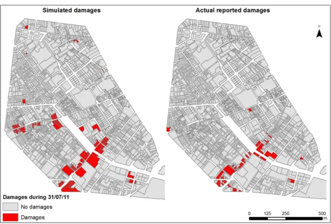
When comparing the actual reported damages with the simulated ones, a few differences were found. The simulated damages were larger, as well as the affected area was. That is why the threshold was increased to 15 cm, meaning that water depths smaller than this value would cause no damages.

(15)

15

Using the curves with this final correction (Figure 2-7), the maps from Figure 2-8 were obtained. Here, the simulated damages (left) and the actual damages reported to the CCS (right), show very similar spatial distributions.

In terms of global damages, the model seems to overestimate the effective damages. Although the values are not coincident, they are within the same order of magnitude and the differences can be explained by the following reasons:

 Due to the methodology followed (presented later in section 2.4.1.3), the damages per each block will be obtained by multiplying the relative cost by its area. When there are very big blocks (as some of the affected ones in Figure 2-8), which may mean that there is only one owner or that it is a cultural or public building, the damages are always overestimated.  Some of the flooded buildings may have not reported their damages to the CCS because

they were small, the property was not insured or they were not aware that they could be compensated.

 The simulated damages are assuming that no flood risk reduction strategies are being used. However, since some of the local population have suffered from previous flood events, it seems reasonable to think that some of them might have protected their assets, by placing wood gates in their doors, or moving the goods to higher areas.

Figure 2-8. Spatial pattern of damages from the 31/07/2011 flood. Simulated damages (left) present very similar pattern than the actual reported damages od the CCS (right).

Although the curves seem to represent accurately (despite the deviations just mentioned) the flood damage processes in the Raval district, they could still be improved. Consequently, whenever more

(16)

16

data is acquired, updates of the curves will be carried out to improve their capacity to represent the real situation of the area.

For example, if long series of damage records are obtained, instead of validating the curves for a given event, the damages could be compared in terms of mean values. Therefore, the mean annual damage recorded could be compared to the simulated EAD.

2.4.1.2.2 Land-use information

As stated previously, good quality and precision of data is crucial when carrying out a micro-scale study. Consequently, regarding land-use, a GIS map has been developed using data from the local land registry at block level (Figure 2-9 left). As the flood typology in the case study area consists in flash floods producing low water depths and high speeds, only land-uses of the ground floor and basements have been added to the dataset.

For each block, more than one land-use type is possible, so the area related to the several land-use types is given. Multiplying these values by the relative damages obtained from the stage-damage curves, the total damages of the block can be obtained. Additionally, it possible to calculate the vulnerability map, which shows the maximum potential damage in monetary units (Figure 2-9 right). As it was previously mentioned, for this vulnerability assessment only six land-use types have been considered. Since the Raval district is a densely populated urban area, there are almost no green or industrial areas (and no agricultural areas at all). Therefore, the uses that have been considered are: (1) warehouses and parkings; (2) commercial; (3) residential; (4) hotels and leisure; (5) public and cultural buildings; and (6) sites of interest. This last category has been introduced because of the special importance of some of the buildings in this specific area, such as museums, churches or historical buildings with inestimable value.

Since the water depth is going to be different depending on the floor level, the land-use maps present this variable into two separate maps. Moreover, from the datasets it is observed that, whereas in the ground level the land-use types are evenly distributed, in the basements there is a predominance of the warehouses and parkings category.

(17)

17

Figure 2-9. Land-use classes in the Raval district, the main land-use class of the ground floor is shown at a block scale (left), and vulnerability map, presenting the potential damage of the assets at risk (right). 2.4.1.3 Risk levels for direct tangible impacts

To integrate the damage modelling with the hydraulic model results, the GIS-based toolbox developed in the frame of WP3 (and described in D3.3) has been particularized for the case of the Raval District.

This version of the toolbox, enables to automatize the three following steps, increasing the speed of the post processing of data and so, easing the simulation of several scenarios:

1. Assign a water depth to each building.

2. Interpolate this value in the stage-damage curve to obtain the relative cost.

3. Multiply the relative cost by the area, obtaining the total damage value per each block. Finally, a shape file with the total damages is obtained, being able to calculate the total costs that have been caused by the extreme rainfall event. This process can be easily repeated for several flood-driven events.

Using this toolbox and the several data described previously, synthetic rain events of 1, 10 and 100 years of return period have been simulated. Then, using the EAD previously defined, an estimate of the current damages in the area has been given.

Using the flood maps presented in Figure 2-6 and the methodology described earlier, flood damage maps are obtained for the studied area (Figure 2-10). As it can be seen in the right map of this figure, some buildings present extremely high damages (more than 200,000 €).

(18)

18

As damage is represented in each block, larger blocks will accordingly present larger damages (as the area flooded will be multiplied by the relative damage to obtain the total figure). This is something which should always be taken into account, because in general, the blocks presenting the highest damage values are also the ones with the largest areas.

From Figure 2-10, the conclusion extracted from the hazard maps (Figure 2-6) is reinforced: the southern and south-western parts of the district are the most vulnerable to floods. Due to the historic characteristic of this region, some particular buildings of inestimable value are located in flood prone areas.

Finally, the EAD of the whole area has been calculated. As it has been stressed before, this value is of high interest as it will be crucial to assess the cost-effectiveness of the adaptation measures proposed. Although this part of the project is still on-going, the baseline scenario to which the rest will be compared has already been determined.

The authors would like to stress that the EAD calculated does not intend to determine the actual damages of the area, but expressing the benefits that could be obtained if some adaptation measures are implemented. In addition, as it was stated previously, the flood maps are an upper bound of the actual situation. Consequently, this methodology will also lead to an overestimation of the damage values. Although this may seem inappropriate, it has been selected as the best hypothesis to allow the identification of the most robust strategies to deal with the impacts of floods.

Figure 2-10. Flood damages in the Raval district for a rain event of return period of 1 year (left), 10 years (centre) and 100 years (right).

In Figure 2-11, the damage – probability curve for the Raval District is presented (for the detailed values, see Table 2-1). In it, the aggregated damages of the entire district are plotted against its probability. As explained before, the area below this curve is the EAD, which has a final value of 1,697,299.8 €. As mentioned, this figure is an overestimation of the annual damage that may be caused by floods in the Raval District, but it provides an estimate of the order of magnitude in which this value ranges.

(19)

19

Figure 2-11. Damage – probability curve for the whole Raval district. The area under this curve expresses the EAD of the region. The probabilities 1, 0.1 and 0.01 represent the events of 1, 10 and 100 years of return period, respectively.

Table 2-1 - Damages and probabilities for the three synthetic rain events simulated.

Return period (years) 1 10 100

Probability 1 0.1 0.01

Damage (€) 78,846 1,615,738 19,156,196

2.4.2 Indirect tangible impacts

The indirect tangible impacts are the ones that can be economically assessed, but which have not been created due to the direct contact with water. Such impacts are the disruption of businesses activities and transport networks, amongst others.

In the Raval District, the flood typology could be defined as flash flooding, with low depths and high velocities. The impacts induced by such floods are localized, and the retention time of the water is generally very short. On the other hand, the Raval District is not crossed by any important communication route, and there are no big commercial or industrial uses within the district.

Consequently, in the area studied the indirect damages will tend to be small compared to the direct ones. Therefore, such damages are not going to be included in this study.

2.4.3 Intangible impacts

As it has been mentioned before, in this case impacts to pedestrians and traffic will be assessed. Since these values will be determined in terms of different risk levels, they are considered in the intangible section.

2.4.3.1 Impacts to pedestrian circulation

2.4.3.1.1 Hazard levels for pedestrian circulation

In order to define specific hazard criteria related to runoff in urban areas, Technical University of Catalonia (Spain) promoted a new research line based on the study of the stability of pedestrians circulating in flooded streets (Russo et al., 2013).

The results of the experimental campaign, presented in terms of flow velocities able to produce critical situations for pedestrian circulation are summarized in the Table 2-2.

(20)

20

Table 2-2. Hazard levels according to flow parameters in flooded streets.

Hazard level Flow conditions

(for flow depths between 9 and 16 cm)

High v  1.88 m/s

Moderate 1.51  v < 1.88 m/s

Low v < 1.51

On the basis of this study, in order to elaborate the hazard maps related to pedestrian circulation for the Barcelona case study, the following high hazard criteria were defined (Figure 22):

- Maximum flow depth ymax = 0.1 m (corresponding to the minimum depth of the kerb of the sidewalks in Barcelona)

- Maximum flow velocity vmax = 1.9 m/s (corresponding to the high hazard level threshold flow velocity for flow depths between 9 and 16 cm).

For the moderate hazard levels the following hazard criteria were adopted:

- Maximum flow depth ymax = 0.06 m (corresponding to a flooded lane 3 m wide with a transverse slope of 2%)

- Maximum flow velocity vmax = 1.5 m/s (corresponding to the moderate hazard level threshold flow velocity for flow depths between 9 and 16 cm).

A GIS post process procedure was applied to adapt the model outputs to the pedestrian flood hazard criteria previously defined. According to it, the hazard map from Figure 2-13 was elaborated for the baseline scenario.

Figure 2-12. Barcelona pedestrian hazard criteria (HH: high hazard; MH: moderate hazard; LH: low hazard).

(21)

21

Figure 2-13. Pedestrian hazard maps of the Raval District for the Baseline Scenario (year 2010). In red high hazard conditions are shown, while in yellow and green colours moderate and low hazard conditions

are represented.

2.4.3.1.2 Vulnerability levels for pedestrian circulation

In order to assess the human vulnerability of the Raval District, statistical data of current and forecasted population in 21 different census areas were used. These data (updated to 2012 and summarized in Table 2-3) were provided by Barcelona municipality and concern:

C: Density of people with critical age: less than 15 years old and more than 65. F: Density of foreign people

D: General people density

B: Presence of critical buildings (such as hospitals, schools, etc.)

Once data were available for the baseline, the following thresholds were defined in order to assess the vulnerability of each census area. Specifically for the human vulnerability related to the people density, thresholds were deduced from the medium density of Barcelona (16000 inhabitants per Km2) and the definition of the National Institute of Statistics of urban area defined as a group of minimum 10 houses in a distance less than 200 m (equivalent to 1273 inhabitants per Km2). The other defined thresholds are shown in Table 2-4.

Three vulnerability indexes were defined according to the 3 first data types and for the final vulnerability index, the average value between C, D and E was computed and in case there was any critical building in the census area, a 0.5 value was added. The final vulnerability level was achieved according to the formulations proposed in the Table 2-5.

(22)

22

Table 2-3. Population data for the baseline scenario.

Table 2-4. Thresholds to assess human vulnerability according to different criteria. Vulnerability

index % people age < 15 C

or > 65 years old F % of foreign people D People density 1 (low) ≤ 33% ≤ 33% ≤ 1273 2 (medium) 33% < X ≤ 50% 33% < X ≤ 50% 1273<X≤16000 3 (high) > 50% > 50% > 16000

Table 2-5. Formulation to compute the total vulnerability index.

Vulnerability level Formulation *

Low (D+C+F)/3 < 1.5

Medium 1.5 < (D+C+F)/3 < 2.5

High D+C+F)/3 > 2.5

*In case there is a critical building is in the subdistrict area, 0.5 must be added to the average value of (D+C+F)/3.

Applying the described methodology, human vulnerability map was obtained for the baseline scenario. In this map, the different vulnerability levels (high, moderate and low vulnerability) of census areas were represented using, respectively red, yellow and green colours (Figure 2-15). Moreover the presence of critical buildings (schools, hospitals, etc.) was also shown in the same map. Census area ID Census area (m2) Total inhabitants (2012) People density

People with age less than 15 years old

People with age more than 65 years old

Foreign people 001 229599 1394 6071 159 229 738 002 38160 1591 41693 190 254 769 003 38992 3365 86300 550 473 1782 004 97356 2868 29459 380 341 1660 005 60933 2637 43277 306 398 1395 006 37115 1875 50519 182 228 846 007 41122 2099 51043 248 171 949 008 35399 3410 96330 477 359 1367 009 26282 2186 83174 235 311 1164 010 27311 2474 90587 348 256 1031 011 37219 3672 98660 517 362 1500 012 23529 1946 82706 220 269 1077 013 16262 1352 83136 152 251 879 014 16530 2038 123289 256 227 1090 015 22182 2307 104003 279 324 1212 016 24590 2332 94835 298 272 1102 017 19584 2769 141389 355 264 1228 018 57310 1554 27116 159 243 872 019 78411 2937 37456 283 367 1404 020 85885 2154 25080 164 408 1461 021 84621 2067 24427 166 330 1314

(23)

23

Figure 2-14. Human vulnerability for the baseline scenario.

2.4.3.1.3 Risk levels for pedestrian circulation

For the flood risk assessment related to pedestrian circulation in the urban areas analysed, the general methodology based on the risk matrix was implemented obtaining the risk for the baseline scenario and the selected return periods. The risk was defined for each census area and represented with the same range of colours previously described.

In order to define the risk level of each census area a statistic treatment of the risk of the cells was carried out. The risk level of each census area was assumed equal to the maximum risk level of the cells, as long as they represented at least a 15% of the total cells located in the same census area. In Figure 2-15 the risk map for the baseline scenario is shown. Obviously, the risk level increases along with the return period.

(24)

24

Figure 2-15. Risk maps for pedestrian related to Baseline scenario and Business as usual scenario for return periods of T = 1, 10 and 100 years.

2.4.3.2 Impacts on vehicles

2.4.3.2.1 Hazard levels for vehicles

A similar procedure to the one defined for pedestrian circulation has been suggested. Stability criteria for stationary vehicles have been defined to create vehicle hazard maps. The conclusions come from a specific report developed by Engineers Australia contracted by Water Research Laboratory: “Appropriate safety criteria for vehicles” (Shand et al. 2010).

This report reviews and discusses previous experimental and analytical investigations of vehicle stability for stationary vehicles (Hydroplaning is therefore not considered further within this study). The two recognized hydrodynamic mechanisms by which stability is lost include buoyancy or floating and friction instability or sliding (Figure 2-16).

Authors of this report finally propose several stability criteria for stationary vehicles that have been summarized in Table 2-6.

(25)

25

Figure 2-16. Hydrodynamic mechanism by which vehicular stability is lost.

Table 2-6. Hazard stability criteria for stationary vehicles.

On the basis of this study, in order to elaborate the hazard maps related to vehicles for the Barcelona case study, the following criteria were adopted (Figure 2-17):

- High hazard criteria were referred to critical flow conditions concerning a vehicle class “Large passenger”. In this case, practically all type of vehicles loss their stability.

- Moderate hazard criteria were referred to critical conditionsconcerning a vehicle class “Small passenger”. In this case, only small cars could loss their stability.

Using these hazard criteria and the results of the models for the baseline scenario, the hazard map for vehicles was elaborated (Figure 2-18). As it can be seen, several streets (above all located in the southern part of the district) could be affected by high flood risk for the return period of 100 years. However, many of these critical streets have little traffic flow as shown in the following vulnerability section concerning traffic flow (Figure 2-19).

(26)

26

Figure 2-17. Hazard criteria for vehicle types in Barcelona case study (HH: high hazard; MH: moderate hazard; LH: low hazard).

Figure 2-18. Vehicle hazard maps for the baseline scenario considering return periods of T = 1, 10 and 100 years. In red high hazard conditions are shown, while in yellow and green colours moderate and low

(27)

27

2.4.3.2.2 Vulnerability levels for traffic

Traffic vulnerability was obtained through assessing the traffic flow data in the Raval district provided by the Traffic Department of Barcelona Municipality. Thresholds were arbitrarily decided based on the average values of the traffic flow in Barcelona streets (Table 2-7). The vulnerability map for traffic is presented in Figure 2-19.

Table 2-7. Vulnerability levels of vehicular circulation.

Vulnerability level Vehicular flow intensity (VFI) (vehicles in 24h)

Low VFI < 5000

Medium 5000 ≤ VFI ≤ 10000

High VFI > 10000

Figure 2-19. Vehicular vulnerability map for the baseline scenario based on traffic intensity (shown values express vehicular flow intensities x 1000 in 24 hours).

2.4.3.2.3 Risk levels for traffic

As applied with the human risk, a matrix combining hazard and vulnerability data for vehicles was implemented for the assessment of vehicular traffic flood risk.

(28)

28

The objective of this step was to determine the risk level of the street on the basis on the hazard levels of each cell and the traffic flow intensity of each traffic lane. Crossing these data and using the risk matrix shown in Figure 2-5, risk maps for vehicular circulation were obtained for the baseline scenario considering the selected return periods (T = 1, 10 and 100 years). They are presented in Figure 2-20.

The streets with high risk for a high return period (100 years) are Ronda de San Pau Street, Parallel Avenue, Rambla del Raval and Pelayo Street (Figure 2-20).

Figure 2-20. Risk maps for pedestrian related to Baseline scenario and Business as usual scenario for return periods of T = 1, 10 and 100 years.

2.5 Discussion and conclusions

In order to improve the capacity to represent urban floods in the Raval District, a 1D/2D coupled model has been developed. The interface between the two drainage layers has been characterized through empirical expressions related to hydraulic performance of surface drainage systems. The 2D domain covers 44 km2 of the city land involving 235 km of sewers, while 2D mesh counts 403,925 triangles.

Calibration and validation of the model is based on the data (rain gauge data, time series of flow depths recorded by water level gauges, reports and videos concerning flooded areas) related to 4 heavy storm events occurred in 2011. The obtained results show that it is possible to reproduce the effects of urban floods in the Raval District in a more realistic way than traditional 1D sewer flow simulations.

(29)

29

With the development of synthetic depth-damage curves regionalized for the case study, an exhaustive economic damage assessment can be carried out when heavy storm events occur. Implementing the described methodology with the GIS-based toolbox, the EAD of the Raval district can be calculated. This enables the determination of the critical points of the district in terms of flooding impacts.

In addition, impacts to pedestrian and vehicular circulation have been assessed, using qualitative methodologies defining several hazard, vulnerability and risk levels. This will allow to be able to assess the benefits of the several adaptation strategies, in non-economic terms.

In the coming months, following the same methodology, several adaptation measures (such as improvements of the sewer network, construction of SUDS or green-roofs, local flood mitigation strategies, etc.) will be simulated. This will allow determining the effectiveness of these strategies in terms of vulnerability reduction, so the ones presenting the best performance can be prioritized over the others.

Currently, the presented data and methodology is ready to be applied, both for the present situation and for the potential future ones, taking into account socio-economic and climatic changes and the implementation of adaptation measures. Even though, this task has not yet been concluded and so, only the baseline scenario has been modelled.

It is worth noting that the damages calculated are an upper bound of the actual damages of the district, because several of the assumptions that have been done are conservative. The aim is to allow determining high robust adaptation strategies that can cope with damages larger than the current ones.

2.6 References for the Barcelona case study

Alcrudo F. and Mulet-Marti J. (2005). Urban inundation models based upon the Shallow Water equations. Numerical and practical issues. Proceedings of Finite Volumes for Complex Applications IV. Problems and Perspectives. Hermes Science publishing. pp 3-1. ISBN 1 905209 48 7.

Gissing, A. & Blong, R. 2004 Accounting for variability in commercial flood damage estimation. Australian Geographer, 35, (2): 209–222.

Godunov S. K. (1959). A Difference Scheme for Numerical Solution of Discontinuous Solution of Hydrodynamic Equations. Math. Sbornik, 47, 271–306, translated US Joint Publ. Res. Service, JPRS 7226, 1969.

Gómez M. and Russo B. (2011). Methodology to estimate hydraulic efficiency of drain inlets. Proceedings of the ICE - Water Management. Institution of Civil Engineers, 164(1), 1-10. Innovyze (2012). InfoWorks ICM (Integrated Catchment Modeling) v.2.5. User manual references. Kok, M., Huizinga, H.J., Vrouwenfelder, A.C.W.M. & Barendregt, A. 2004 Standard Method 2004.

Damage and casualties caused by flooding. Client: Highway and Hydraulic Engineering Department.

(30)

30

Manojlovic N., & Pasche, E. 2010 Theory and Technology to Improve Stakeholder Participation in the development of Flood Resilient Cities, Proc. Int. 21st IAPS Conference on Vulnerability, Risk and Complexity: Impacts of Global Change on Human Habitats, Leipzig, Germany.

Merz, B., Kreibich, H., Schwarze, R. & Thieken, A. 2010 Review article: assessment of economic flood damage. Natural Hazards and Earth System Science, 10, 8, 1697-1724.

Messner, F., Penning-Rowsell, E., Green, C., Meyer, V., Tunstall, S. & Van der Veen, A. 2007 Evaluating flood damages: guidance and recommendations on principles and methods. FLOODsite Project.

Nascimento, N., Machado, M. L., Baptista, M. & Silva, A. D. P. 2007 The assessment of damage caused by floods in the Brazilian context. Urban water journal, 4, 195-210.

Penning-Rowsell, E., Johnson, C., Tunstall, S., Tapsell, S., Morris, J., Chatterton, J. B. & Green, C. 2005 The benefits of flood and coastal risk management: a manual of assessment techniques, Middlesex University Press.

Reese, S., Markau, H.J. & Sterr, H. 2003 MERK – Mikroskalige Evaluation der Risiken in überflutungsgefährdeten Küstenniederungen. Abschlussbericht. Kiel.

Russo B., Suñer D., Velasco M. and Djordjević S. 2012. Flood hazard assessment in the Raval District of Barcelona using a 1D/2D coupled model.9th International Conference on Urban Drainage Modelling. Belgrado, Serbia. ISBN 978-86-7518-155-2.

Russo B., Gómez M. And Macchione F. 2013. Pedestrian hazard criteria for flooded urban areas. Natural Hazards. Springer. 63(11), 2666-2673. DOI: 10.1007/s11069-013-0702-2.

Shand T. D., Cox R. C., Blacka M. J., Smith G. B. 2011. Appropriate Safety Criteria for Vehicles. Literature Review. Stage 2 Report, Australian rainfall and runoff Project 10. Engineering Australia, Water Engineering.

Thieken, A.H., Müller, M., Kreibich, H. & Merz, B. 2005 Flood damage and influencing factors: New insights from the August 2002 flood in Germany. Water Resources Research, 41, (12).

(31)

31

3 Case study Beijing

3.1 Case study area overview

The Beijing case study looks at the flooding impacts at various scales. Although a city-wide hydraulic model in coarse resolution has been developed (See D2.4) for the central Beijing city, the detailed land use information are not available for the central Beijing area such that the flood damage cannot be evaluated at the city-wide scale. Instead, the new urban development area Yizhuang was used for damage assessment.

Yizhuang is a satellite town in the south of Beijing. It has been quickly developed in the last two decades with population grew from 104,000 in 2001 to 700,000 in 2012. Yizhuang has attracted huge investment and the Beijing city government has provided detailed information, including terrain model, land uses and sewer network, that we can use in the CORFU project. These data are utilised in the hydraulic model, together with the current rainfall patterns, to simulate the flooding in Yizhuang. The results are combined with the land uses estimate the flood damage for the baseline scenario.

For the central Beijing city, we have learnt that the traffic disruption during flooding is more critical than the tangible damage to buildings. Most of the disruptions were caused by flooding at the under bridge tunnels. The terrain and the poor drainage in those areas resulted in flooding that affected the traffic significantly when heavy rainfall occurred. Many of the under bridge tunnels are located at the junctions of trunk roads such that the ripple effect often spreads widely and stalled the traffic in the main road networks. To investigate the influence of flooding on the traffic, we built a detailed hydraulic model for the under bridge tunnels (See D2.4) to simulate the dynamic of flooding at such locations. For the impact assessment, we collected the related traffic information for Beijing and tried to develop a traffic model using the software called SUMO. Nevertheless, the SUMO software requires some essential car journeys information that were not yet available. Hence, we gathered other related information on population, car journeys, and the road network from public websites. In February 2012, the number of vehicles in Beijing reached 5 million (http://auto.sina.com.cn/service/2012-02-17/0704918344.shtml) and 70% of those are private vehicles. The average traffic in central Beijing (inner 6th ring road) is 30 million passengers/day in 2012 (8.3 million via buses or trams, 5.1million via subways, 9.9million by private cars, 2 million by taxis, and 4.2million by bicycles) (Beijing Transportation Research Centre, 2013, Year book of traffic development in Beijing city, 2013).

With hydraulic modelling results for the central Beijing area, the flood hotspots of those under bridge tunnels will be identified. With the detailed hydraulic model of the bridge areas, the flood extents, depth and duration will be simulated such that the triggers for traffic disruption can be properly established in the SUMO model for traffic modelling. The results will be compared to the baseline model with normal traffic condition such the influence of flooding on the traffic at the city-wide scale can be evaluated (in terms of extra journey time, consumption of fuel, or loss of working hours, etc.).

(32)

32

3.2 Scenarios

The impact assessment described in this deliverable is calculated for a single scenario: the present-day situation. Future deliverables will provide the impact assessment results that have been undertaken assuming different future scenarios (D3.8) and different measures and strategies (D3.9).

3.3 Hydraulic modelling

Pipe network data, ground elevation data and rainfall information are the three essential components for the hydraulic model. The drainage network data includes topology, structure of the pipes, pumping stations, relevant hydraulic facilities and other hydrological and hydraulic parameters. The surface information contains catchment processes parameters and a ground digital elevation model, for which a 10m*10m regular grid model is generated for the case study. The rainfall information is the input for 1D network modelling, combined with Beijing annual maximum storm intensity formula and 24-h hydrological hyetograph to generate design rainfall for various return periods. The hydraulic modelling results have been provided in D2.4.

3.4 Damage / impact modelling

Building content flood damage evaluation typically encompasses four steps: hazard analysis, bearing body exposure assessment, vulnerability analysis and loss quantification. Firstly, hazard analysis is the process of acquiring information such as indictor intensity, frequency and scope, and hydraulic model to execute scenario analysis becomes the mainstream direction. The premise for constructing urban flooding model is to gather detailed information of drainage network, river, drainage structures, ground surface and rainfall, which could be achieved by remote sensing analysis and site survey. Based on a series of hydrology and hydraulic principles, this numerical model simulates physical process of flood occurrence and evolution to obtain hazard indicators variation over time and space. Secondly, through socio-economic survey and statistics and geospatial information database, the exposure assessment takes advantage of area weighting method to derive spatial attributes of socio-economic condition, thereby reflecting spatial distribution difference in the economic indicator of bearing body. Lastly, vulnerability analysis, usually represented by depth- damage curve, relies on the typical sampling survey to establish statistical relationship between hazard and economic losses factors. In view of above statement, the flood damage assessment procedure is demonstrated in Figure 3-1.

(33)

33

Figure 3-1 Flood damage assessment procedure

The vulnerability expression could be identified as relationships between hazard and loss rate or absolute loss value. The depth-absolute loss vulnerability curves of various types of assets have been set up in large amount of developed countries, but the loss rate is more preferred in China. In fact, these two approaches just differ slightly in expression manner but with same essence. Due to the association between the building land use type and loss rate, the following formula is generated to calculate flood damage.

 



 i j ij i j L L  ,

Where L is total flood loss, is loss value of property category at depth j, is the loss rate of property category at depth .

Deriving water depth-damage curve of buildings which fits local economic development situation is basic for implementing loss and risk evaluation. Based on synthesis assumption analysis of indoor property value, part of building depth-damage curves of Beijing has been constructed, which is based on 10 types of land use according to the flood damage database of UK (Penning Rowsell et al, 2010) as shown in Figure 3-2.

Remote Sensing Analysis

Site Survey Hydraulic Model Hazard Indicator (Intensity,Frequency,Scope) Socio-economic Survey Socio-economic Statistic Geospatial information Exposure Assessment (Land use,Value,Distribution)

Typical losses survey

vulnerability analysis (Loss rate,Absolute loss)

Loss Quantification

(34)

34

Figure 3-2 UK Depth-damage curves

Building vector data were collected for the case study. Each building has a unique index value is introduced to distinguish building vector data, which could be overlain with land use maps to generate the building land use spatial distribution (Figure 3-3).

Figure 3-3 Building land use spatial distribution

To deal with direct flood damage evaluation, WP 3 has developed a tool using Python script and the ArcObjects, the geoprocessing functions within the ESRI ArcGIS software, which can evaluate the damage directly from the hydraulic model results. This tool is capable of exerting flood damage calculation and risk analysis with spatial properties at single building scale (Figure 3-4 Building damage results of (a)10, (b)20, (c)50, and (d)100 year return period of rainfall event). The flood damage statistics is summarized in Table 3-1.

Table 3-1 Flood damage and rainfall statistics for different return periods

Return period (year) 10 20 50 100

Rainfall(mm) 172 197 229 254

Total Loss(hundred million RMB) 2.01 3.23 4.97 5.90

Flood Depth(m) Fl o o d D a m a g e( G D P p er m 2) Residential

Manufacturing and Processing Commercial

Service activities Education and research Government services Recreational facilities Mixed use Transport services Parking lots Residential

Manufacturing and Processing Commercial

Service activities Education and research Government services Recreational facilities Mixed use Transport services Parking lots Green spaces Water body Cropland Unused area

(35)

35

Figure 3-4 Building damage results of (a)10, (b)20, (c)50, and (d)100 year return period of rainfall events

The relationship of flood damage versus design storm frequency is shown in Figure 3-5.

Figure 3-5 Relationship of flood damage versus design storm frequency Indirect tangible impacts 3.4.1 Traffic impact modelling

An assessment of indirect tangible impacts will be made by an analysis of the impacts of flooding on traffic through disruption. Traffic disruption results from reduced vehicle speeds and blockage of traffic at critical spots. This problem occurs frequently in Beijing. A serious storm hit Beijing in June

0 50 100 150 200 250 300 1 2 3 4 5 6 7 8 9 0 0.02 0.04 0.06 0.08 0.1 0.12 hu nd re d m ill ion R M B Frequency

Total Loss (hundred million RMB) Rainfall(mm)

(36)

36

23, 2011. It disrupted the whole traffic system in BeijingFigure 3-6 presents data on the traffic condition from that event. Green represents ‘good’ traffic condition, and black in completely blocked. The other colours represent different conditions, depending on the road type. The classification is presented in Table 3-2. Another serious storm hit Beijing in July 21 2012. It again disrupted the whole traffic system in Beijing and more than 70 people were killed by flooding. Data from that storm are presented in Figure 3-7. Impacts on traffic are represented in Figure 3-8Figure 3-8 Impacts on traffic in Beijing, July 23, 2012

Figure 3-6 Impacts on traffic and real time traffic situation in Beijing, June 23, 2011

Table 3-2 Classification for the traffic map colours

Classification Grade Design Speed _（

km/h） Colour Traffic speed （km/h） Fast road Ⅰ 100 Green >65 Ⅱ 80 Yellow (50，65] Ⅲ 60 Red ≦50 Trunk road Ⅰ 60 Green >45 Ⅱ 50 Yellow (25，45] Ⅲ 40 Red ≦25 Secondary road Ⅰ 50 Green >35 Ⅱ 40 Yellow (15，35] Ⅲ 30 Red ≦15 Branch Ⅰ 40 Green Ⅱ 30 Yellow Ⅲ 20 Red

(37)

37 Figure 3-7 Storm with spatiotemporal distribution in Beijing

Figure 3-8 Impacts on traffic in Beijing, July 23, 2012

After July 21 2012, Beijing News reported that the city's water authority admitted the shortcomings of its infrastructure, but experts said it would take time to upgrade Beijing's flood protection systems.

Figure 3-9 show the road maps of Beijing and Figure 3-10 shows the example of the detail information for the road database. The traffic models, such as VlSSIM (Germany), CORSIM, Synchro/SimTraffic and TransModeler (USA), Paramics (UK), AIMSUN (Spain) and DYNAMEQ

(38)

38

(Canada) are used in China. We adopted SUMO to simulate the traffic in Beijing. The data were converted to create a SUMO traffic model for the Beijing city, as shown in Figure 3-11.

Figure 3-9. Road map

(39)

39

Figure 3-11. SUMO model for the traffic in Beijing city

The impacts of rainfall on traffic have been identified in two aspects. One is the significant negative changes of road condition and visibility during the rain events process, another is adverse effects of the residue accumulated on the road resulted from the extreme rainfall.

In the operation process of urban transportation, the velocity of vehicles is reduced. Especially for the locations where traffic intensive and water accumulated, traffic congestion and paralysis possibly occur, which is one of the important indicators to justify the impacts of flood on traffic. Since it is difficult to express the influence by mathematical model, this research takes into account the effects of water inundation to road and focuses on the derivation of mathematical model. The following model analysis regards the normal operation status of urban traffic as reference. The attenuation model of traffic velocity with water depth is illustrated in the following formula:

0 _tanh( ₎ 0 2 2 v x a v v b    

Where v is the velocity of vehicles (km/h), v0 is design velocity of vehicles which varies according to the road grade (km/h), x is the accumulated water depth (cm), a is critical water depth that results vehicles stopped (cm), b is the coefficient of attenuation which identifies the decreasing rate of velocity versus depth, the range 3-5 (the smaller of b, the faster of declining).

Table 3-3 Traffic loss categories due to excessive rainfall

Aspects of impacts Types of loss Categories of loss

Economy

Direct loss Loss of fuel consumption Z1 Loss of time consuming Z2 Indirect loss Loss of personal working hours Z3

Loss of infrastructure destruction Z4

Politics and Society Indirect lossZ5 The political effects of major events and the dissatisfying of residence to municipal facilities

(40)

40 Total traffic loss Z=Z1+Z2+Z3+Z4+Z5

The economic loss due to extra fuel consumption could be calculated by the relationship between velocity of vehicles and fuel usage. The velocity of traffic is decreased by water inundation, which is less than the critical velocity with minimum fuel consumption. Based on mechanical theory, the losses raised by fuel consumption could be acquired by the following formula:

1 1

1

1 (

)

70

n b

Pe be

Z

v













Where Pe is the power of engine (KW), be is the efficiency of fuel consumption (g/KW/h), vb is

critical vehicles velocity with minimum fuel consumption (km/h), is the unit price of fuel (RMB/L), n is the influenced traffic by flood inundation.

The economic loss of time consuming could be get according to the following formula:

2 1 2

Z



M



M

M1 is economic loss of time consuming of private car: 1 1 1 1 n i M 



  t



m

M2 is economic loss of time consuming of motor coach: 2 2 2 2 n i M 



  t  m

Where:



t

is the duration of damage (h) which could be get through site survey or estimated by average duration of public travelling, is evaluation indicator of time value (RMB/h),

m

1is the average seating numbers of private car 1.5-2,

m

2is the average seating numbers of motor coach 40-80,n1 and n2 are traffic numbers of private cars and motor coach respectively in the survey area. The traffic simulation model could be constructed after collection and rearrangement of basic dada for study area, while the parameters for calculating traffic loss is able to derive from the model by appropriate assumption input (e.g. the number of influenced vehicles). However, due to the deficiency of basic data, this part of work is still on-going.

3.5 Discussion and conclusions

For Beijing case study, currently only the depth-damage curves regarding residential building have been synthesized, depth-damage curves of other building types are still on the process. Therefore, the information extracted from UK flood damage database is adopted for the case study of Yizhuang. Due to the diversification of regional economic circumstances, the outcome of flood loss in this case is relatively magnified compared to actual status. The approaches of traffic loss evaluation have

(41)

41

been generated. Owning to the deficiency of data required for traffic simulation model, for instance traffic load and road condition information, the process of constructing traffic model is not implemented at the moment. However, the construction and initial calibration of hydraulic model for 20 bridges in Beijing has been completed. The next step will place emphasis on collecting basic traffic data and implementing traffic evaluation of specific Beijing case study based on urban local flood model.

Flood Damage Model Case Study Results

Work Package:

Document Name:

Flood Damage Model Case Study Results

Date:

11 August 2014

Report Number:

D3.4

Revision Number:

2

Deliverable Number:

D3.4

Due date for deliverable:

31 December 2011

Actual submission date:

15 August 2014

Author:

University of Exeter

Document Dissemination: PU (Publically disseminated)

DOCUMENT INFORMATION:

Title

Flood Damage Model Case Study Results

Lead Authors

Michael Hammond, Albert Chen, Slobodan Djordjevic

Contributors

David Butler, Marc Velasco, Beniamino Russo, David Khan, Jelena

Batica, Kapil Gupta, Yuwen Zhou, Natasa Manojlovic, Ming-Hsi Hsu

Distribution

PU - Public

Document

Reference

DOCUMENT HISTORY:

01 July 2012

Contents

1

Introduction

2

Case study Barcelona

2.1

Case study area overview

2.2

Scenarios

2.3

Hydraulic modelling

2.4

Damage / impact modelling

1

2

3

1

1

2

3

2

2

4

6

3

3

6

9

Hazard

V

ul

ne

ra

bi

li

ty

Risk Matrix

2.5

Discussion and conclusions

2.6

References for the Barcelona case study

3

Case study Beijing

3.1

Case study area overview

3.2

Scenarios