Hyperdimensional Computing-based Multimodality Emotion Recognition with Physiological Signals

This is the post peer-review accepted manuscript of:

E. Chang, A. Rahimi, L. Benini and A. A. Wu, "Hyperdimensional Computing-based

Multimodality Emotion Recognition with Physiological Signals," 2019 IEEE

International Conference on Artificial Intelligence Circuits and Systems (AICAS),

Hsinchu, Taiwan, 2019, pp. 137-141.

The published version is available online at:

https://ieeexplore.ieee.org/document/8771622

© 2019 IEEE. Personal use of this material is permitted. Permission from IEEE must be obtained for all other

uses, in any current or future media, including reprinting/republishing this material for advertising or

promotional purposes, creating new collective works, for resale or redistribution to servers or lists, or reuse

of any copyrighted component of this work in other works.

Hyperdimensional Computing-based Multimodality

Emotion Recognition with Physiological Signals

En-Jui Chang

, Abbas Rahimi

, Luca Benini

, and An-Yeu (Andy) Wu

a

_{Integrated System Laboratory, ETH Zurich;}

_{University of Bologna;}

_{National Taiwan University}

{

echang, abbas, lbenini

}

@iis.ee.ethz.ch, [email protected]

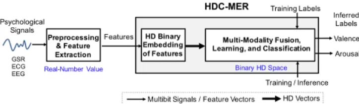
Abstract—To interact naturally and achieve mutual sympathy between humans and machines, emotion recognition is one of the most important function to realize advanced human-computer interaction devices. Due to the high correlation between emotion and involuntary physiological changes, physiological signals are a prime candidate for emotion analysis. However, due to the need of a huge amount of training data for a high-quality machine learning model, computational complexity becomes a major bottleneck. To overcome this issue, brain-inspired hyperdimensional (HD) computing, an energy-efficient and fast learning computational paradigm, has a high potential to achieve a balance between accuracy and the amount of necessary training data. We propose an HD Computing-based Multimodality Emotion Recognition (MER). HDC-MER maps real-valued features to binary HD vectors using a random nonlinear function, and further encodes them over time, and fuses across different modalities including GSR, ECG, and EEG. The experimental results show that, compared to the best method using the full training data, HDC-MER achieves higher classification accuracy for both valence (83.2% vs. 80.1%) and arousal (70.1% vs. 68.4%) using only1/4training data. HDC-MER also achieves at least 5% higher averaged accuracy compared to all the other methods inany point along the learning curve.

Index Terms—Hyperdimensional computing, affective computing, emotion recognition, physiological signal processing

I. INTRODUCTION

Affective computing is emotional artificial intelligence that can recognize, realize, and respond to human affect, which is a key technology to build cognitive human–computer interfaces in the era of Internet of Things (IoT) [1]. A wide range of potential applications of affective computing have been proposed, including driver warning systems, automated tutoring systems, and health care systems [2], [3]. Therefore, to accurately interpret human emotions, their recognition is one of the most important functions in affective computing.

Emotion is a subjective mental state caused by some specific events that is usually accompanied by characteristic behaviours and involuntary physiological changes. General approaches of emotion recognition commonly gather data from faces and voices to measure human emotions [4], [5]. However, the emotions are not always expressed through facial expression or voice. Unlike these controllable signals, physiological signals are spontaneous and not controlled by the subject, some of which become useful inputs for enhancing emotion analysis. Moreover, as intelligent IoT continues to advance, more and more wearable devices are equipped with different kinds of sensors that continuously monitor and collect various signals sensed from subjects. Recent machine learning-based methods are proposed to use these physiological This research was supported in part by the Ministry of Science and Technology of Taiwan (MOST 107-2917-I-564-038), the ETHZ Postdoctoral Fellowship Program, and the EU’s H2020 under grant No. 780215.

Preprocessing & Feature Extraction

Psychological Signals

HDC-MER Training Labels Inferred

Labels

Real-Number Value Binary HD Space

Features

GSR ECG EEG

Multi-Modality Fusion, Learning, and Classification HD Binary

Embedding of Features

HD Vectors Multibit Signals / Feature Vectors

Training / Inference Valence Arousal

Fig. 1. HD computing-based multi-modality emotion recognition framework.

signals to improve the accuracy of emotion recognition. The state-of-the-art (SoA) methods include Bayes classifier [6]–[9], support vector machine (SVM) [8]–[10], and extreme gradient boosting (XGB) [10].

However, these SoA methods require a large amount of train-ing data for a high-quality machine learntrain-ing model. Moreover, their computational complexity is a major bottleneck for their real-time execution on wearable devices. Specialized architec-tures for machine learning can boost energy efficiency towards TOPS/Watt [11], but further improvement requires a novel look at data representations, associated operations, circuits, and at ma-terials and substrates that enable them [12]. Novel brain-inspired computational paradigms that support fast learning could lead the way: hyperdimensional (HD) computing [13]—an emerging computational framework based on computing with random HD vectors—provides energy-efficient, robust, and fast learning [14]– [20]. HD computing demonstrates fast learning in various biosig-nal processing tasks [14]–[16], each of which operates with a specific type of biosignals (see [17] for an overview). In this paper, we extend HD computing for multimodal sensor fusion from different types of physiological signals. This paper makes the following contributions:

• We propose HDC-MER1 as an HD computing-based

mul-timodal emotion recognition from galvanic skin response (GSR), electrocardiographic (ECG), and electroencephalo-graphic (EEG) recordings. Such fusion of information and scalability to different modalities is achieved by a robust, distributed, HD vector representation that allows multiple alternatives to be superposed over the same HD vector and processed as a single unit. To jointly monitor the different aspects of physiological changes, HDC-MER fuses the

features from all modalities to a compositeHD vector that

is further processed for learning and inference.

• We propose a simple embedding that maps a real-valued

feature to a binary HD vector that modulated by a sparse random HD vector. This embedding expands the original 1_{Source codes are available at http://github.com/enjui/HDC-MER}

feature representation into a higher dimensional binary rep-resentation, in an unsupervised fashion, using a randomly generated nonlinear function to set every component of the HD vector.

• HDC-MER optimizes the number of taps in the temporal

encoder to capture the meaningful time-dependent emotional fluctuations for better learning quality. HDC-MER surpasses the SoA methods in both speed of learning and classification accuracy. Compared to XGB using the full training data, HDC-MER achieves higher classification accuracy for both valence (84.9% vs. 80.1%) and arousal (70.1% vs. 68.4%)

using only 1/4 training data. HDC-MER also achieves at

least 5% higher averaged accuracy compared to all the SoA

methods in any point along the learning curveconfirming

its superior accuracy with arbitrary amount of training data.

II. RELATEDWORK ANDBACKGROUND

A. Related Work of Emotion Recognition with Biosignals

Basic human emotion can be described as a circumplex model [21]. This model suggests that emotions are distributed in a two-dimensional circular space, including valence and arousal. Valence describes how positive or negative the emotion is, and arousal indicates the intensity of emotion. Based on this model, affective states can be represented at any level of valence and arousal. For example, the excitation is a high-arousal and positive-valence state, and the depression is a low-arousal and negative-valence state.

A common machine-learning-based emotion recognition con-sists of signal preprocessing, feature extraction, and classification. Input data are physiological signals, and output are the results of classification for valence and arousal. To improve the accuracy of classification, most related works focus on how to process physiological signals effectively and extract features from dif-ferent modalities. Additionally, emotion-related factors, such as personality and mood, are also discussed in the related works. ASCERTAIN [8] examines the relationship between emotion and personality traits via users’ physiological responses and classifies the emotion by using Naive Bayes (NB) and SVM. AMIGOS [9] provides a dataset for the affect research as well as applies Gaussian Naive Bayes (GaussianNB) and SVM for the emotion classification. Moreover, to measure the complexity of physiological signals, the entropy-assisted approach [10] was proposed to extracts the entropy domain features to quantify the regularity and randomness of signal. In [10], the schemes of emotion recognition based on SVM and XGB also were implemented. However, these SoA methods require large amount of data for training, and impose high computational complexity that hinder their application for resource-limited wearable devices.

B. Background of HD Computing

The operation of the human brain relies on billions of neurons and synapses, suggesting that massive neural activities are fun-damental to its computational power. Brain-inspired HD comput-ing [13] aims to model the neural activity patterns by computcomput-ing with vectors in a very high (e.g., thousands) dimensionality called HD vectors. Hence, distributed data representation with HD vectors is the core of HD computing. Namely, any item can be represented as an HD vector where independent and

identically distributed components do not have specific meaning.

With dimensionality (d) of 10,000, there are billions of nearly

orthogonal HD vectors. This enables HD computing to combine two such HD vectors into a new HD vector using well-defined vector space operations, while keeping the representative infor-mation of the original two HD vectors with high probability. Other leading properties of HD computing includes robustness, energy efficiency, massively parallel operations, and fast one-shot learning [12]. These make it well-suited for efficient biosignal

processing [17], e.g., 2×lower energy at iso-accuracy when

com-pared to a highly-optimized SVM on an ARM Cortex M4 [15]. Larger energy saving is achieved by using emerging 3D nanoscale devices [18], [19]. HD computing has been applied to various learning and multiclass inference tasks, such as the language identification [22], [23], EMG gesture recognition [14], [15], EEG-based brain–machine interfaces [16], and in general ExG processing [17].

As a hardware-friendly coding for HD computing, we focus on binary dense codes [12] where the components of HD vectors are

binary with equally probable1s and0s (see [20], [23] for binary

sparse code and related operations). Using the dense binary code, arithmetic operations in the HD space simply involve bitwise addition, multiplication, and permutation, defined as follow:

• Addition: The sum of two HD vectorsAandBis denoted as

[A+B]and defined as the componentwise majority function

with ties broken at random, also called as bundling. Bundling two HD vectors produces a new HD vector that is similar to both input HD vectors. Therefore, it is well-suited for representing sets.

• Multiplication: The product of two HD vectorsA andB is

denoted asA⊕Band defined as the componentwise XOR. It

generates a dissimilar HD vector to the corresponding input HD vectors and is suited for variable binding.

• Permutation: It shuffles the components of an HD vectorA

by one-bit cyclic right shifting, denoted asρ(A). Permutation

produces a dissimilar HD vector, which is good for encoding a sequence.

HD computing starts by generating a set of seed HD vectors

in an item memory (IM) to represent basic items defined in the system. These seeds can be combined to encode a composite HD vector using the aforementioned operations to represent an event of interest. This composite HD vector can be stored, or make incremental updates, in an associative memory (AM) during learning; it can also be compared (using Hamming distance) with already learned HD vectors during classification.

III. PROPOSEDHDC-MER SCHEME

The proposed HDC-MER scheme consists of 1) HD binary embedding of features, and 2) multimodality fusion, learning, and classification in the HD space, as shown in Fig. 2. The features of GSR, ECG, and EEG are inputs. In this work, we use the same preprocessing and features in [10] to extract 214 features (i.e., GSR:32, ECG:77, EEG:105) based on statistical and frequency domain. These multimodal features include 1) GSR: skin response/conductance and skin conductance slow response, 2) ECG: heart rate variability and heart rate time series, 3) EEG: average power spectral density of theta band, alpha band, beta band, and gamma band. All features are normalized to a range

from −1 to +1. This work does binary classification for both valence and arousal. Thus, HDC-MER returns two labels as

outputs per trial for the positive/negative valence (i.e., V+ or

V−) and high/low arousal (i.e., Ah _{or A}l_{), respectively.}

A. HD Embeddings with Random Nonlinearity

The main goal of our embedding is to represent a real-valued feature with a binary HD vector. In Fig. 2, two inputs from a feature, i.e., its actual values and its unique identifier (ID), are mapped from the original representation to the HD representation. An ID of a feature is treated as a basic field, and its value is viewed as the filler of this field.

We propose a simple function that nonlinearly maps a

real-valued feature to a sparse HD vector where the number of1s is

much lower than the number of 0s. The nonlinear behaviour is

randomly but programmatically inscribed based on the HD vector component that the function operates with. The detailed execution of our mapping is as follows:

• Step 1. For mapping every feature value (vi), we use a

randomSi vector. LetSi be ad-dimensional sparse ternary

vector where its j-th element is denoted by sij. These

elements are independent random variables with probability distribution defined as:

sij =      +1 with probability(1−p)/2 0 with probability p −1 with probability(1−p)/2 i∈ {1, ..., m}, j∈ {1, ..., d}

wheremis the number of features, dis the dimensionality

of embedding, and pis a sparsity factor (i.e., probability of

0s).

• Step 2. We set each bit of the embedding HD vector (bij)

based on the sign of product between the feature value,vi∈

[−1,+1], andsij as: bij =

(

1 if vi·sij >0

0 if vi·sij ≤0

Therefore, the value of a feature is mapped to a d-bit sparse

HD vector that is denoted asσ(vi×Si). For a hardware-friendly

design, the HD embeddings can be equivalently implemented by

multiplexers with three input HD vectorsS_i+, S_i−, and S0

i. The

selection signal is the sign of feature valuevi. For example, when

vi >0, the positive vector Si+ (i.e., b(Si+ 1)/2c) is selected.

Besides mapping the value of a feature, its ID is also mapped to

a unique HD vectorDi via the IM. In contrast, the IM maps the

IDs to dense HD vectors that are nearly orthogonal. Binding an ID

of a feature to its value in the HD space,Di⊕σ(vi×Si), produces

another dense HD vector. This resulting HD vector can be readily used by the arithmetic operations for dense coding in the next stage. In other words, our embedding maps the entire range of

every normalized float featurevito three dense binary HD vectors

whose relative distances can be controlled byp(derived fromDi

and modulated by one ofS_i+,S_i−,S0

i).

B. Multimodality Fusion, Learning, and Classification

After embedding, the generated HD vectors are sent, sequen-cilly, to the spatial encoder, temporal encoder, fusion unit, and

𝜌Permutation HD Binary Embedding of Features Feature 1 Feature 32 … ID … 𝜌 Spatial HD Encoder Temporal HD Encoder GSR Path ECG Path EEG Path

Multimodality Fusion, Learning, and Classification Associative Memory Prototype HD Vectors (V+, V-) ( Ah, A l) Query HD Vectors Hamming Distance Training/Inference Training Labels Inferred Labels F HD Fusion Unit HD Vectors Multibit Signals / Feature Vectors

σ(𝝊𝟑𝟐𝒕 x 𝑺𝟑𝟐) TGSR TEEG TECG [+] σ(𝝊𝟏𝒕x 𝑺𝟏) Rt GSR [+] D Multiplication [+] Addition Valence Arousal Item Memory value D1 𝑺𝟏( 𝑺_𝟏𝟎 𝑺𝟏* Item Memory value D32 𝑺_𝟑𝟐( 𝑺𝟑𝟐𝟎 𝑺𝟑𝟐* ID =0 <0 >0 =0 <0 >0 𝝊_𝟑𝟐𝒕 𝝊_𝟏𝒕

Fig. 2. The block diagram of HDC-MER.

AM for learning and classification. Firstly, the spatial encoder bundles the information across all features of a modality at a

given time point t. It is done by applying the majority function

among the components of HD vectors. For example in GSR, it is given by:

Rt_GSR= [(σ(vt₁×S1)⊕D1) +...+ (σ(vt32×S32)⊕D32)] Secondly, the emotion is continuously changing over time. Therefore, the temporal encoder is applied to capture the changes of features between videos (i.e., the stimuli to evoke the emotion of a subject) to capture the time-dependent emotional fluctuation. By using permutation operation, the temporal encoder can

gener-ate ann-gram HD vector based on a sequence ofnfeatures [17],

which can be derived as ad-bit temporal HD vector:

TGSR = n Y

t=1

ρt−1Rt_GSR

After the encoding in spatial and temporal domain, the next step is to fuse the multimodal HD vectors. To keep representative information from all modalities, the fusion unit bundles the

corresponding HD vectors as a fusedd-bit HD vector:

F = [TGSR+TECG+TEEG]

Then, this output of fusion unit (F) is sent to the AM for the

training and inference. During the training phase, F generated

from the training data is bundled to its corresponding class

prototype in the AM. That is, AM collects all F of the same

class and bundles them to a prototype HD vector by the majority

function. For example, the prototype HD vectorP of V+_{can be}

given by:

PV+= [F_{1st trial}+...+F_{last trial}]

Therefore, after the training, there are in total four prototype

HD vectors in the AM for V+, V−, Ah, and Al. During the

inference phase we use the same encoding but the label of F

is unknown, hence we call it the query HD vector. To perform classification, the query HD vector is compared with all learned prototype HD vectors to identify its source class according to the Hamming distance (i.e., the measure of similarity), defined as the number of bits that differ between the two HD vectors. Finally, two emotional labels with the minimum distance are returned.

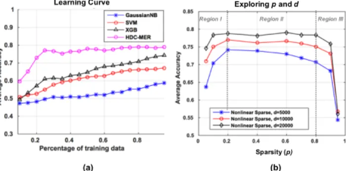
(a) (b)

Learning Curve Exploring pand d

Sparsity (p)

Region III Region I Region II

Fig. 3. (a) The comparison of learning curve among GaussiianNB, SVM, XGB, and HDC-MER. (b) The accuracy of HD embeddings with different sparsity. (region I: uncorrelated modulation, region II: effective modulation, region III: correlated modulation)

IV. EXPERIMENTALSETTINGS ANDRESULTS

A. Dataset and Simulation Settings

We use the physiological signals provided from AMIGOS dataset [9] to generate the corresponding features by means of a 30 s window by sliding over 15 s. There are in total 33 subjects and 16 short-length videos in the database after removing outliers [10]. Each recording contains 1 channel for GSR, 2 channels for ECG, and 14 channels for EEG. Leave-one-subject-out method is conducted to evaluate the performance, and the final performance is calculated by the averaging method.

B. Analysis ofn-gram and Learning Curve

Firstly, to capture the significant period of emotional

fluctu-ation, we have to determine the proper size of an n-gram to

represent the affective state. In this work, whenn-gram is 4, the

accuracy of valence and arousal can achieve the highest value of 0.832 and 0.701, respectively. This means that a sequence of 4 feature windows (i.e., 75 s signals) is to be formed as a rep-resentative HD vector to capture temporal correlations. Notably,

increasing then-gram does not bring accuracy improvements, due

to the long-term uncorrelated data that are out of 75 s period. Fig. 3(a) compares the learning curve among GaussianNB [6], SVM [9], XGB [10] and HDC-MER. As the amount of training data increases, the average accuracy of valence and arousal grows gradually. When using 25% of the total dataset for training, the average accuracy of HDC-MER reaches 76.6%, with an improvement of at least 16.2% compared to the SoA classifiers. Although the accuracy can be improved by increasing the training data for all the methods, the learning curve of HDC-MER is always superior to the others After using 25% of training data, the accuracy of HDC-MER is almost saturated. This is in contrast with the other methods that require further training to improve their accuracy. In all the points along the learning curve, HDC-MER achieves the highest accuracy.

C. Accuracy Analysis with Different Levels of Sparsity

Fig. 3(b) shows the average accuracy of our embedding with

different sparsity (pvalues) and dimensionality (d={5000, 10000,

20000}). Notably, varying sparsity for the HD embedding is a way

to change distances between Di and the modulated HD vectors

(Di⊕σ(vi×Si)). The HD embedding with a higherpkeeps more

elements ofDiunchanged and bypasses them to the next stage. In

TABLE I

ACCURACY FOR DIFFERENTEMOTIONRECOGNITIONSCHEMES Classifiers Accuracy

GSR ECG EEG All

V GaussianNBa 0.538 0.543 0.585 0.588 SVMa 0.640 0.615 0.589 0.680 XGBa _{0.776 0.634 0.581 0.801} HDC-MERb 0.822 0.628 0.626 0.832 A GaussianNBa _{0.553 0.561 0.598 0.589} SVMa 0.644 0.623 0.566 0.663 XGBa 0.682 0.542 0.579 0.684 HDC-MERb _{0.694 0.614 0.661 0.701}

a _{Learning Fraction=97%}b_{Learning Fraction=25%,p=0.7}

contrast, the HD embedding with a lowerpcan flip more elements

of Di, which increases the distance. Therefore, according to the

different range of p in Fig. 3(b), we can further define three

regions to qualitatively describe those relative distances: region I (p <0.2) as uncorrelated modulation, region II (p= 0.2–0.8)

as effective modulation, and region III (p > 0.8) as correlated

modulation. In the region I, the accuracy quickly increases with

lower dimensionality of d=5000. In the region II, the accuracy

falls slightly from 0.748 (p=0.2) to 0.710 (p=0.8). Afterp=0.8, it

keeps dropping to around 0.55 due to the close distance between modulated HD vectors. Similarly with higher dimensionality of

d={10000, 20000}, the accuracy degrades considerably in region

I and III. In contrast, in region II, the accuracy remains stable

within a range of ±0.016. Therefore, to keep the accuracy high

and stable, we can choosep=0.2–0.8 with higher dimensionality

for HDC-MER. In this paper, we use p=0.7 and d=10000 to

analyze accuracy for different scenarios of modalities in the next section.

D. Accuracy Analysis for Different Scenarios of Modalities

Table I shows the comparison of accuracy with four scenarios, including only GSR, or ECG, or EEG, and all the modalities. Using all the modalities, HDC-MER can improve the accuracy of valence by 3.1%–24.4% and arousal by 1.7%–11.2% with

only1/4 of training data. In addition, HDC-MER outperforms

the other three classifiers in almost every scenario. Notably, the arousal can be improved by up to 9.5% with only unimodal EEG features, and the maximal improvement of valence is 28.4% by only using GSR features. It implies that each modality provides different information for the emotional intensity and reaction. Therefore, by using the multimodal HD fusion, HDC-MER can achieve the highest accuracy for valence and arousal.

V. CONCLUSIONS

This paper presents HDC-MER that jointly considers multi-modal fusion of physiological signals and a sequence of features to represent the temporal aspect of emotion for the accuracy im-provement. Additionally, HDC-MER effectively maps features of biosignals to binary HD vectors, and quickly learns a meaningful pattern for classification with fewer training data. Based on our experimental results, HDC-MER achieves the highest average classification accuracy up to 76.6% with the fastest learning among all the existing emotion recognition schemes.

REFERENCES

[1] R. W. Picard, “Affecting computing for HCI,” in

Proc.8th International Conf.Human−Computing Interaction, pp. 829-833, 1999.

[2] D. Katsis, N. S. Katertsidis, G. Ganiatsas, and D. I. Fotiadis, “Toward emotion recognition in car-racing drivers: A biosignal processing approach,” IEEE Trans.Syst., Man, Cybern.A,Syst., Humans, vol. 38, no. 3, pp. 502512, May 2008.

[3] D. Katsis, N. S. Katertsidis, and D. I. Fotiadis, “An integrated system based on physiological signals for the assessment of affective states in patients with anxiety disorders,” Biomed.Signal Process.Control, vol. 6, pp. 261268, 2011.

[4] S. Shojaeilangari, W.-Y. Yau, K. Nandakumar, J. Li, and E. K. Teoh, “Robust representation and recognition of facial emotions using extreme sparse learning,”IEEE Trans.Image Processing, vol. 24, no. 7, pp. 21402152, Jul. 2015.

[5] V. Vielzeuf, C. Kervadec, S. Pateux, A. Lechervy, and F. Jurie, “An Occams razor view on learning audiovisual emotion recognition with small training sets,” ArXiv e-prints, 2018.

[6] S. Koelstra, C. Muhl, M. Soleymani, J. S. Lee, A. Yazdani, T. Ebrahimi, T. Pun, A. Nijholt, and I. Patras, “DEAP: A database for emotion analysis using physiological signals,”IEEE Trans.Affective Computing, vol. 3, no. 1, pp. 18-31, Jan.-March, 2012.

[7] G. Valenza, A. Lanata, and E.P. Scilingo, “The role of

nonlinear dynamics in affective valence and arousal recognition,”

IEEE Trans.Affective Computing, vol. 3, no. 2, pp. 237249, Apr.Jun. 2012.

[8] R. Subramanian, J. Wache, M. Abadi, R. Vieriu, S. Winkler, and N. Sebe, “ASCERTAIN: emotion and personality recognition using commercial sensors,”IEEE Trans.Affective Computing, vol. 9, no. 2, pp.147-160, Apr.-Jun., 2018.

[9] J.A. Miranda-Correa, M.K. Abadi, N. Sebe, and I. Patras, “AMIGOS: A dataset for mood, personality and affect research on individuals and groups,” IEEE Trans. Affective Computing, vol.pp, no.99, Nov. 2018.

[10] S.-H. Wang, H.-T. Li, E.-J. Chang, and A.-Y. (Andy) Wu, “Entropy-assisted emotion recognition of valence and arousal using XGBoost clas-sifier,” in Proc. 14th International Conf. Artificial Intelligence Applications and Innovations (AIAI), pp. 249-260, 2018.

[11] B. Moons, R. Uytterhoeven, W. Dehaene, and M. Verhelst, “14.5 envision: A 0.26-to-10tops/w subword-parallel dynamic-voltage-accuracy-frequency-scalable convolutional neural network processor in 28nm FDSOI,” in2017 IEEE International Solid-State Circuits Conference (ISSCC), Feb 2017, pp. 246–247.

[12] A. Rahimi, S. Datta, D. Kleyko, E.P. Frady, B. Olshausen, P. Kanerva, and J.M. Rabaey, “High-dimensional computing as a nanoscalable paradigm,” IEEE Trans.Circuits and Systems I: Regular Papers, vol. 64, no. 9, pp. 2508-2521, 2017.

[13] P. Kanerva, “Hyperdimensional computing: An introduction to comput-ing in distributed representation with high-dimensional random vectors,” Cognitive Computation, vol. 1, no. 2, pp. 139159, 2009.

[14] A. Rahimi, S. Benatti, P. Kanerva, L. Benini, and

J.M. Rabaey, “Hyperdimensional biosignal processing: A

case study for EMG-based hand gesture recognition,” in

Proc.IEEE International Conf.Rebooting Computing, Oct. 2016.

[15] F. Montagna, A. Rahimi, S. Benatti, D. Rossi, and L. Benini, “PULP-HD: accelerating brain-inspired high-dimensional computing on a parallel ultra-low power platform,” inProc.Design Automation Conf., 2018.

[16] A. Rahimi, P. Kanerva, J. del R. Mill´an, and J.M. Rabaey,

“Hyperdimensional computing for noninvasive braincomputer

interfaces: Blind and one-shot classification of EEG error-related

potentials,” in Proc. 10th ACM/EAI International Conf. Bio−

inspired Information and Communications Technologies(BICT), 2017.

[17] A. Rahimi, P. Kanerva, L. Benini, and J. M. Rabaey, “Efficient Biosignal Processing Using Hyperdimensional Computing: Network Templates for Combined Learning and Classification of ExG Signals,” inProceedings of the IEEE, 2018.

[18] T. F. Wu, et al., “Brain-inspired computing exploiting carbon nanotube FETs and resistive RAM: Hyperdimensional computing case study,” in2018 IEEE International Solid - State Circuits Conference (ISSCC), Feb 2018, pp. 492– 494.

[19] H. Li, et al., “Hyperdimensional computing with 3D VRRAM in-memory kernels: Device-architecture co-design for energy-efficient, error-resilient language recognition,” in2016 IEEE International Electron Devices Meeting (IEDM), Dec 2016, pp. 16.1.1–16.1.4.

[20] D. Kleyko, A. Rahimi, D.A. Rachkovskij, E. Osipov, and J.M.

Rabaey, “Classification and recall with binary hyperdimensional com-puting: tradeoffs in choice of density and mapping characteristics,”

IEEE Trans.Neural Networks and Learning Systems, vol. PP, no. 99, pp. 1-19, 2018.

[21] J. Posner, J. Russell, and B. Peterson, “The Circumplex Model of Affect: An Integrative Approach to Affective Neuroscience, Cognitive Development, and Psychopathology,”Development and Psychopathology, vol. 17, no. 3, pp. 715-734, 2005.

[22] A. Joshi, J. T. Halseth, and P. Kanerva, “Language geometry

using random indexing,” in Proc.10th International Symp.

Quantum Interaction(QI), pp. 265274, 2016.

[23] M. Imani, A. Rahimi, J. Hwang, T. Rosing, J. M. Rabaey, “Low-Power

Sparse Hyperdimensional Encoder for Language Recognition,” in IEEE