Shifted Linear Interpolation Filter

Shifted Linear Interpolation Filter

H. Olkkonen1, J. T. Olkkonen2

1

Department of Physics and Mathematics, University of Eastern Finland, Kuopio, Finland, 2VTT Technical Research Centre of Finland, VTT, Finland

Email: [email protected], [email protected]

Received September 21st, 2010; revised November 8th, 2010; accepted November 15th, 2010.

ABSTRACT

Linear interpolation has been adapted in many signal and image processing applications due to its simple implementa-tion and low computaimplementa-tional cost. In standard linear interpolaimplementa-tion the kernel is the second order B-spline β2

 

t . In this

work we show that the interpolation error can be remarkably diminished by using the time-shifted B-spline β2



t -Δ



as

an interpolation kernel. We verify by experimental tests that the optimal shift is Δ=0.25. In VLSI and microprocessor

circuits the shifted linear interpolation (SLI) algorithm can be effectively implemented by the z-transform filter. The

interpolation error of the SLI filter is comparable to the more elaborate higher order cubic convolution interpolation.

Keywords: Linear Interpolation, Cubic Convolution, B-splines, VLSI

1. Introduction

Linear interpolation plays an important role in modern signal and image processing applications due to its sim-ple imsim-plementation and low computational cost. Plonka [1,2] has extensively studied the effect of the shifted in-terpolation nodes on the approximation error in the B- spline interpolation. According to the theoretical analysis the shift 0 yields the minimal error norm. Blu et al. [3] applied the same idea to the piecewise-linear interpo-lation. On the contrary, they observed that interpolation error diminishes if the sampling knots are shifted by a fixed amount. Through the theoretical considerations Blu

et al. [3] determined the optimal shift of the knots is close to  1 / 5 of the distance between the knots.

In this work we consider a modification of the linear interpolation. In standard linear interpolation the kernel is the second order B-spline 2( )t . Instead of shifting

the sampling knots we introduce the shifted linear inter-polation (SLI), where the B-spline kernel has been time-shifted by a fraction  of the sampling period. We describe the z-transform SLI filter for efficient imple-mentation of the shifted B-spline kernel 2(t )

es-pecially for VLSI and microprocessor circuits.

2. Theoretical Considerations

2.1. B-Spline Signal Processing

B-spline approximation of the continuous signal x t

 

is based on the summation [4]

 

 

p





k

x t 



c k  t k (1)

where c k

 

are the scale coefficients. The B-spline

 

p t

 is constructed by convolving an indicator

func-tion 

 

t by itself

 

   

 

p times

p t t t t

   

 (2)

where

1 0 1

( )

0 elsewhere

t t

 _{ }  

 (3)

The linear interpolation is obtained in the case p2

 

 

2





k

x t 



c k  t k (4)

where 2

 

t is the triangle function Figure 1 defined as

2

for 0 t<1

( ) 2 for 1 t 2

0 elsewhere

t t

t t



 



   

 

(5)

2.2. Shifted Linear Interpolation

Let us consider the approximation of the continuous-time signalx t

 

by a summation of the shifted B-spline





2 t

  

 

 

, 2





k

x t 



c  k  t  k (6)

[image:2.595.68.286.85.257.2]

Shifted Linear Interpolation Filter 45

Figure 1. The shifted B-spline 2



t 



.

where c

 

,k , 

 

0,1 is the scale sequence for the time-shifted kernel. In the sequel we call (6) the shifted linear interpolation (SLI). Usually the data points are known in discrete time intervals tnT n



0,1, 2,



. In the z-transform domain we obtain

 

 

 















 



2

1 ,

, 1

Z x n X z C z Z t

C z z





    

 

  _     _ (7)

The SLI filter is now obtained from (6) as











 

 



1

, 1

Z x n d_{ }C _ z _{   }d _{  }d z _

  (8)

By inserting the scale sequence C



,z



from (7) we finally have











 



 



  

1

1 1

1 , ,

d d z

Z x n d X z

z SLI d z X z





     

 

   

 

(9)

where SLI d



, , z



denotes the SLI filter.

2.3. Inverse SLI Filter

In some applications it is required that the original signal has to be reconstructed from the delayed one. In the gen-eral case the SLI filter (9) has no stable inverse since the roots of the nominator may lie outside the unit circle. For

0.25

  the roots are inside the unit circle in the range

0 d 0.25. The inverse SLI filter can be realized by the inverse filtering procedure described in Appendix I.

3. Experimental

3.1. Experimental Verification of the SLI Algorithm

We tested experimentally the quality of the SLI filter for a variety of synthetic signals with varying frequency components. The interpolation error was defined as the absolute difference between the analytically calculated and interpolated signal: e t

 

 x t

 

xint

 

t . The time-

shift of the interpolation kernel was altered in the range

0  1. The interpolation error was strongly related to the time-shift. Irrespective of the type of the signal the minimum interpolation error was obtained in every case at  0.25. Figure 2 shows an example of the interpo-lation error versus  for signal sin 0.1



t



, when

0.5

d . The worst case is the linear interpolation

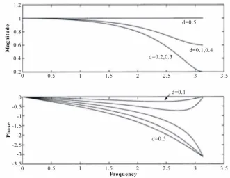
[image:2.595.163.435.474.682.2]

[image:3.595.134.465.85.341.2]

Figure 3. The magnitude and phase responses of the SLI filter for d =0.1,,0.5



Δ= 0.25



.



 0



. Then the interpolation error diminishes from

0.21

  to  0.25. At bigger  values the inter-polation error starts to increase.

The magnitude and phase response of the SLI filter is given in Figure 3 for  0.25 and d0.1,, 0.5. Magnitude response of the SLI filter decreases at higher frequency values, albeit in the case d0.5 the magni-tude is constant in the whole frequency range. The phase shift is linear in the frequency range0  1. For

0.5

d and  0.25 the magnitude response of the

SLI filter turns to high-pass and tends to intensify the noise occurring in high frequency range. As a practical solution the interpolated signal can be time-reversed and 1d can be inserted instead of d in the SLI algo-rithm.

3.2. Half Delay Filter

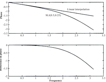
An interesting application of the SLI is the half delay filter, which delays the signal half of the sampling period and interpolates the intermediate points between the evenly spaced knots. For  0.25 and d0.5 we have



  

_{ }

11 1 3 0.5, 0.25,

1 1 3

z

SLI z

z



  

 (10)

which is an all-pass filter having the unity magnitude response. The interpolation error of the half delayed filter (11) is especially low Figure 2. Figure 4 shows the

phase response and the phase error compared with the ideal phase response.

3.3. Comparison with the Cubic Convolution Interpolation

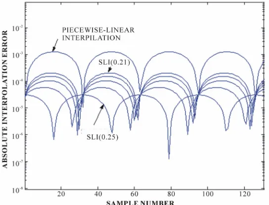
The absolute interpolation error using the cubic convolu-tion method [5] and the SLI-algorithm for signals

 

sin

 

x n  n and x n

 

sin 2

 

n are given in Fig-sures 5 and 6 for d = 0.5 and  0.25. At 1 the cubic convolution interpolation performs slightly better, but at 2 the quality of the SLI algorithm equals the cubic convolution.

4. Discussion

[image:4.595.119.483.90.374.2]

Shifted Linear Interpolation Filter 47

[image:4.595.310.533.416.595.2]

Figure 4. Comparison of the phase responses of the piecewise-linear interpolation and the SLI filter(d = 0.5, Δ=0.25).

Figure 5. The absolute interpolation error yielded by the SLI algorithm (d = 0.5, Δ=0.25) and the cubic convolu-tion interpolaconvolu-tion for the sinusoidal signalx n = sin n

 

 

. cubic convolution method is significantly higher com-pared with the SLI algorithm.

The interpolation function used as a kernel in the SLI algorithm correspond the B-spline order p = 2 Figure 1. The B-spline 2

 

t has the z-transform





1 1   z .

Figure 6. The absolute interpolation error yielded by the SLI algorithm (d = 0.5, Δ=0.25) and the cubic convolu-tion interpolaconvolu-tion for the sinusoidal signal

 

 

2

x n = sin n .

[image:4.595.60.282.417.594.2]

sur-prising experimental observation of the SLI algorithm is the strong dependence of the interpolation error on the time shift . Our comparisons using a variety of func-tions with different waveforms and frequency content showed that every time the interpolation error attains its

minimum at  0.25. Previously Plonka [1,2] has

studied the B-spline interpolation with shifted nodes. In the theoretical analysis the shift parameter 0

yielded the minimal error norm. Blu et al. [3] conducted theoretically the piecewise-linear interpolation error ver-sus the shift in the measurement knots. Their analysis predicted the optimal choice  0.21. Blu et al. [3] used a pre-filter to shift the measurement knots and then the standard piecewise linear interpolation for computa-tion of the interpolated signal. An advantage in this pro-cedure is that the prefiltered signal can be directly im-plemented by any existing linear interpolation hardware, while the implementation of the SLI filter needs a new hardware design.

An essential observation in this work is that the SLI filter has low-pass frequency response characteristics only in the range 0 d 0.5. For d0.5 the fre-quency response of the SLI filter turns to high-pass and intensifies the noise occurring in high frequency range. The noise interference for d0.5 can be avoided by time reversing the interpolated signal. Then 1d can be inserted instead of d in the SLI algorithm.

A shortcoming in the SLI algorithm is the phase error occurring in the high frequency range compared with the linear interpolation. Fortunately, in most of the signal processing applications the signal is band limited and the high frequency band 2  contains only some noise components.

An interesting observation is that for d0.5 and

0.25

  the half delay SLI algorithm reduces to the

simple all-pass filter (10), which has the unity magnitude response and the phase response is close to the ideal phase response in the range 0  1. If the signal bandwidth is limited to this range the SLI algorithm yields interpolation precision and accuracy, which is comparable to the more elaborate interpolation methods. The interpolation of intermediate points between the uniformly distributed knots is probably the most fre-quently used operation is image and signal processing. The half delay filters are also important tools in con-struction of shift invariant wavelet transform [9]. The half delay SLI filter (10) can be readily applied to replace the more elaborate half delay filters based on the Thiran filters [10]. For 0 d 0.25and  0.25the SLI filter has a stable inverse. If the original data points have to be reconstructed from the interpolated ones, the inverse SLI filter for higher values of d can be realized by using the

inverse filtering procedure (Appendix I).

5. Conclusions

In signal and image processing applications linear inter-polationhas been frequently used due to its simple im-plementation and low computational cost. In standard linear interpolation the kernel is the second order B-spline 2

 

t . We show in this work that the interpo-lation error can be remarkably reduced by adapting the time-shifted B-spline 2



t 



as an interpolation ker-nel. By experimental tests we verify that the optimal shift is  0.25. The shifted linear interpolation (SLI) algo-rithm can be effectively implemented by the z-transform filter in VLSI and microprocessor applications. The in-terpolation error of the SLI filter is comparable to the more elaborate cubic convolution interpolation. The fu-ture research goal is to extend the time-shifted interpola-tion kernel to higher order B-splines.

Appendix I. Implementation of the inverse fil-terSLI1



d, , z



for  0.25 and d0.25.

By denoting the interpolated signal by

 









Y z Z x n d the inverse filter SLI1



d, , z



is





_

_{ }

1

_

_{ }

 

1 1 1 , , 1 X z z

SLI d z

Y z

d d z

                (11) The inverse filterSLI1



d, , z



is not stable which is not stable for  0.25 and d 0.25 , since the root in the denominator is outside the unit circle. However, the inverse filter can be implemented by the following inverse filtering procedure. First we replace z by z-1





_{ }

 

1

_

_{ }





1

_

1 1 1 1 1 , , 1

X z z

SLI d z

d d z

Y z  _                  (12)

The inverse filter SLI1



d, , z1



is stable for

0.25

  and d 0.25 . The X z

 

1 and Y z

 

1 are the z-transforms of the time reversed signal





x N n and the interpolated signal y N n







. The

following Matlab program ISLI.m demonstrates the

computation procedure. function x = ISLI(y,d,delta) y = y(end:-1:1);

x = filter([delta 1-delta],[delta+d 1-delta-d],y); x = x(end:-1:1);

REFERENCES

[1] G. Plonka, “Periodic Spline Interpolation with Shifted Nodes,” Journal of Approximation Theory, Vol. 76, No. 1, 1994, pp. 1-20.

Shifted Linear Interpolation Filter 49

pp. 297-316.

[3] I. J. Schoenberg, “Contribution to the Problem of Ap-proximation of Equidistant Data by Analytic Functions,” Quarterly of Applied Mathematics, Vol. 4, No. 1, 1946, pp. 45-99, 112-141.

[4] T. Blu, P. Thevenaz and M. Unser, “Linear interpolation revitalized”, IEEE Trans. Image Process. Vol. 13, No. 5, pp. 710-719, May 2004.

[5] R. G. Kay, “Cubic Convolution Interpolation for Digital Image Processing,” IEEE Transactions on Acoustics, Speech, Signal Processing, Vol. 29, No. 6, December 1981, pp. 1153-1160.

[6] P. Thevenaz, T. Blu and M. Unser, “Interpolation Revis-ited,”IEEE Transactions on Medical Imaging, Vol. 19, No. 7, July 2000, pp. 739-758.

[7] J. T. Olkkonen and H. Olkkonen, “Fractional Delay Filter Based on B-Spline Transform,” IEEE Signal Processing Letters, Vol. 14, No. 2, February 2007, pp. 97-100. [8] J. T. Olkkonen and H. Olkkonen, “Fractional Time-Shift

B-Spline Filter,” IEEE Signal Processing Letters, Vol. 14, No. 10, October 2007, pp. 688-691.

[9] H. Olkkonen and J. T. Olkkonen, “Half Delay B-Spline Filter for Construction of Shift Invariant Wavelet Trans-form,” IEEE Transactions on Circuits and Systems II,

Vol. 54, No. 7, July 2007, pp. 611-615.