DIFFUSIONS
A. DE GREGORIO AND S.M. IACUS
Abstract. The aim of this paper is to introduce a new type of test statistic for simple null hypothesis on one-dimensional ergodic diffusion processes sampled at discrete times. We deal with a quasi-likelihood approach for stochastic differential equations (i.e. local gaussian ap-proximation of the transition functions) and define a test statistic by means of the empirical L2-distance between quasi-likelihoods. We prove that the introduced test statistic is asymp-totically distribution free; namely it weakly converges to aχ2 random variable. Furthermore, we study the power under local alternatives of the parametric test. We show by the Monte Carlo analysis that, in the small sample case, the introduced test seems to perform better than other tests proposed in literature.
Keywords: asymptotic distribution free test, local alternatives, maximum-likelihood type es-timator, discrete observations, quasi-likelihood function, stochastic differential equation.
1. Introduction
Let (Ω,F,F = (Ft)t≥0, P) be a filtered complete probability space. Let us consider a
1-dimensional processesX = (Xt)t≥0solution to the following stochastic differential equation
(1.1) dXt=b(α, Xt)dt+σ(β, Xt)dWt, X0=x0,
where x0 is a deterministic initial value. We assume thatb: Θα×R→R,σ: Θβ×R→Rare Borel known functions (up toαandβ) and (Wt)t≥0is a one-dimensional standardFt-Brownian motion. Furthermore,α∈Θα⊂Rm1, β∈Θ
β⊂Rm2, m
1, m2∈N,are unknown parameters and
θ = (α, β)∈Θ := Θα×Θβ, where Θ represents a compact subset of Rm1+m2. We denote by θ0:= (α0, β0) the true value ofθand assume thatθ0∈Int(Θ).
The sample path of X is observed only at n+ 1 equidistant discrete times tni, such that
tn
i −tni−1= ∆n<∞fori= 1, ..., n,(withtn0 = 0). Therefore the data, denoted by (Xtn i)0≤i≤n,
are the discrete observations of the sample path of X. Let p be an integer with p ≥ 2. The asymptotic scheme adopted in this paper is the following: T =n∆n→ ∞, ∆n→0 andn∆pn →0 asn→ ∞. This scheme is called rapidly increasing design, i.e. the number of observations grows over time but no so fast.
This setting is useful, for instance, in the analysis of financial time series. In mathematical finance and econometric theory, diffusion processes described by the stochastic differential equa-tions (1.1) play a central role. Indeed, they have been used to model the behavior of stock prices, exchange rates and interest rates. The underlying stochastic evolution of the financial assets can be thought continuous in time, although the data are always recorded at discrete instants (e.g. weekly, daily or each minute). For these reasons, the estimation problems for discretely observed stochastic differential equations have been tackled by many authors with different approaches (see, for instance, [10], [33], [11], [5], [23], [24], [2], [12], [18], [3], [6], [29], [34], [30], [26], [31], [20]). For clustering time series arising from discrete observations of diffusion processes [7] propose a
Date: May 28, 2018.
new dissimilarity measure based on theL1 distance between the Markov operators. The
change-point problem in the diffusion term of a stochastic differential equation has been considered in [6] and [16]. In [15], the authors faced the estimation problem for hidden diffusion processes ob-served at discrete times. An adaptive Lasso-type estimator is proposed in [8]. For the simulation and the practical implementation of the statistical inference for stochastic differential equations see [13], [14] and [17].
We also recall that the statistical inference for continuously observed ergodic diffusions is a well-developed research topic; on this point the reader can consult [25].
The main object of interest of the present paper is the problem of testing parametric hy-potheses for diffusion processes from discrete observations. This research topic is less developed in literature. It is well-known that for testing two simple alternative hypotheses, the Neyman-Pearson lemma provides a procedure based on the likelihood ratio which leads to the uniformly most powerful test. In the other cases uniformly most powerful tests do not exist and for this reason the research of new criteria is justified.
For discretely observed stochastic differential equations, [21] introduced and studied the as-ymptotic behavior of three kinds of test statistics: likelihood ratio type test statistic, Wald type test statistic and Rao’s score type test statistic.
Another possible approach is based on the divergences. Indeed, several statistical divergence measures (which are not necessarily a metric) and distances have been introduced in order to decide if two probability distributions are close or far. The main goal of this metric is to make “easy to distinguish” between a pair of distributions which are far from each other than between those which are closer. These tools have been used for testing hypotheses in parametric models. The reader can consult on this point, for example, [27] and [28]. For stochastic differential equations sampled at discrete times, [9] introduced a family of test statistics (for p = 2 and
n∆2n→0) based on empiricalφ-divergences.
We consider the following hypotheses testing problem concerning the vector parameterθ H0:θ=θ0, vs H1:θ6=θ0,
and assume thatX is observed at discrete times; that is the data (Xtn
i)0≤i≤n are available. In
this work we study different test statistics with respect to those used in [9] and [21]. Indeed, the purpose of this paper is to propose a methodology based on a suitable “distance” between the approximated transition functions. This idea follows from the observation that in the case of continuous observations of (1.1), we could define the L2-distance between the continuous
loglikelihood. Clearly this approach is not useful in our framework and then, similarly to the aforementioned papers, we consider the local gaussian approximation of the transition density of the processX from Xti−1 to Xti. In other words, we resort the quasi-likelihood function
intro-duced in [23], defined by means of an approximation with higher order correction terms to relax the condition of convergence of ∆n to zero. Therefore, letlp,i(θ), θ∈Θ, be the approximated log-transition function fromXti−1 toXti representing the parametric model (1.1). We deal with
Dp,n(θ1, θ2) := 1 n n X i=1 [lp,i(θ1)−lp,i(θ2)]2, θ1, θ2∈Θ,
which can be interpreted as the empiricalL2-distance between two loglikelihoods. If ˆθ
p,n is the maximum quasi-likelihood estimator introduced in [23], we are able to prove that, underH0,the
test statistic
Tp,n(ˆθp,n, θ0) :=nDp,n(ˆθp,n, θ0)
is asymptotically distribution free; i.e. it converges in distribution to a chi squared random variable. Furthermore, we study the power function of the test under local alternatives.
The paper is organized as follows. Section 2 contains the notations and the assumptions of the paper. The contrast function arising from the quasi-likelihood approach is briefly discussed in Section 3. In the same section we define the maximum quasi-likelihood estimator and recall its main asymptotic properties. In Section 4 we introduce and study a test statistic for the hypotheses problem H0 : θ = θ0 vs H1 : θ 6= θ0. The proposed new test statistic shares the
same asymptotic properties of the other test statistics presented in the literature. Therefore, to justify its use in practice among its competitors, a numerical study is included in Section 5 which contains a comparison of several test statistics in the “small sample” case, i.e., when the asymptotic conditions are not met. Our numerical analysis shows that, at least forp= 2,the performance of test statistic T2,n is very good. The proofs are collected in Section 6.
It is worth to point out that for the sake of simplicity in this paper a 1-dimensional diffusion is treated. Nevertheless, it is possible to extend our methodology to the multidimensional stochastic differential equations setting.
2. Notations and assumptions Throughout this paper, we will use the following notation.
• θ:= (α, β) andα0, β0 andθ0 denote the true values ofα, βandθ respectively. • c(β, x) =σ2(β, x).
• C is a positive constant. IfC depends on a fixed quantity, for instance an integerk,we may writeCk. • ∂αh := ∂ ∂αh, ∂βk := ∂ ∂βk, ∂ 2 αhαk := ∂2 ∂αh∂αk, h, k = 1, ..., m1, ∂ 2 βhβk := ∂2 ∂βh∂βk, h, k = 1, ..., m2, ∂α2hβk := ∂2 ∂αh∂βk, h = 1, ..., m1, k = 1, ..., m2, ∂θ := (∂α, ∂β) 0, where ∂ α := (∂α1, ..., ∂αm1) 0 and∂ β:= (∂β1, ..., ∂βm2) 0, ∂2 θ := [∂ 2 αjβk]h=1,...,m1,k=1,...,m2.
• Iff : Θ×R→R,we denote byfi−1(θ) the valuef(θ, Xtn
i−1); for instancec(β, Xtni−1) = ci−1(β).
• For 0≤i≤n, tni :=i∆n andGin:=σ(Ws, s≤tni).
• The random sample is given byXn := (Xtn
i)0≤i≤n andXi:=Xtni.
• The probability law of (1.1) is denoted byPθandEθi−1[·] :=Eθ[·|Gin−1].We setP0:=Pθ0
andE0i−1[·] :=Eθi−1 0 [·]. • Pθ −→ n→∞and d −→
n→∞stand for the convergence in probability and in distribution, respectively.
• LetFn: Θ×Rn→RandF : Θ→R; “Fn(θ,Xn) Pθ −→
n→∞F(θ) uniformly in θ” stands for
sup θ∈Θ |Fn(θ,Xn)−F(θ)| Pθ −→ n→∞0. Furthermore, ifFn(θ,Xn) Pθ −→ n→∞0 uniformly inθwe set Fn(θ,Xn) =oPθ(1).
• Letunbe aR-valued sequence. We indicate byRa function Θ×R2→Rfor which there exists a constantC such that
R(θ, un, x)≤unC(1 +|x|)C, for allθ∈Θ, x∈R2, n∈N. Let us setRi−1(∆kn) :=R(θ,∆ k n, Xi−1). • For am×nmatrixA,||A||2= tr(AA0) =Pm i=1 Pn j=1|Aij|2. LetC↑k,h(R×Θ;R) be the space of all functionsf such that:
(ii) f(θ, x) is continuously differentiable with respect toxup to orderk≥1 for all θ; these
x-derivatives up to order kare of polynomial growth inx,uniformly inθ;
(iii) f(θ, x) and allx-derivatives up to orderk≥1,areh≥1 times continuously differentiable with respect to θ for all x∈ R. Moreover, these derivatives up to the h-th order with respect toθ are of polynomial growth inx,uniformly inθ.
We need some standard assumptions on the regularity of the processX. A1. (Existence and Uniqueness) There exists a constantC such that
sup α∈Θα
|b(α, x)−b(α, y)|+ sup β∈Θβ
|σ(β, x)−σ(β, y)| ≤C|x−y|.
A2. (Ergodicity) The process X is ergodic for θ = θ0 with invariant probability measure
π0(dx). Thus 1 T Z T 0 f(Xt)dt Pθ −→ T→∞ Z f(x)π0(dx),
wheref ∈L1(π0). Furthermore, we assume thatπ0 admits all moments finite.
A3. infx,βσ(β, x)>0.
A4. (Moments) For allq≥0 and for allθ∈Θ, suptE|Xt|q<∞.
A5. [k] (Smoothness)b∈C
k,3
↑ (Θα×R,R) andσ∈C↑k,3(Θβ×R,R).
A6. (Identifiability) If the coefficients b(α, x) = b(α0, x) and σ(β, x) = σ(β0, x) for all x
(π0-almost surely), thenα=α0and β=β0.
LetLθ the infinitesimal generator ofX with domain given byC2(R) (the space of the twice continuously differentiable function onR); that is iff ∈C2(R)
Lθf(x) :=b(α, x) ∂f ∂x(x) + c(β, x) 2 ∂2f ∂x2(x), L0:=Lθ0.
Under the assumption A5[2(j−1)] we can define L
j θ := Lθ◦L j−1 θ with domain C 2j( R) and L0 θ=Id.
We conclude this section with some well-known examples of ergodic diffusion processes be-longing to the class (1.1):
• the Ornstein-Uhlenbeck or Vasicek model is the unique solution to (2.1) dXt=α1(α2−Xt)dt+β1dWt, X0=x0,
where b(α1, α2, x) = α1(α2−x) and σ(β1, x) = β1 with α1, α2 ∈ R and β1 > 0. This
stochastic process is a Gaussian process and it is often used in finance where β1 is the
volatility, α2 is the long-run equilibrium of the model and α1 is the speed of mean
reversion. For α1 >0 the Vasicek process is ergodic with invariant law π0 given by a
Gaussian law with meanα2 and variance
β2 1
2α1.It is easy to check that all the conditions A1−A6 fulfill;
• the Cox-Ingersoll-Ross (CIR) process is the solution to (2.2) dXt=α1(α2−Xt)dt+β1 p XtdWt, X0=x0>0, whereb(α1, α2, x) =α1(α2−x) andσ(β1, x) =β1 √ xwithα1, α2, β1>0.If 2α1α2> β12
the process is strictly positive, otherwise non negative. This model has a conditional density given by the non central χ2 distribution. The CIR process is useful in the
description of short-term interest rates and admits invariant lawπ0 given by a Gamma
distribution with shape parameter 2α1α2
β2 1
and scale parameter β12
2α1. If (2.2) is strictly
3. Preliminaries on the quasi-likelihood function
We briefly recall the quasi-likelihood function introduced by [23] based on the Itˆo-Taylor expansion. The main problem in the statistical analysis of the diffusion process X is that its transition density is in general unknown and then the likelihood function is unknown as well. To overcome this difficulty one can discretizes the sample path ofX by means of Euler-Maruyama’s scheme; namely Xi−Xi−1= Z tni tn i−1 b(α, Xs)ds+ Z tni tn i−1 σ(β, Xs)dWs'bi−1(α)∆n+σi−1(β)(Wtn i −Wtni−1). (3.1)
Hence (3.1) leads to consider a local-Gaussian approximation to the transition density; that is L(Xi|Xi−1)'N(bi−1(α)∆n, ci−1(β)∆n)
and the approximated loglikelihood function of the random sampleXn,called quasi-loglikelihood function, becomes (3.2) ln(θ) := 1 2 n X i=1 (X i−Xi−1−bi−1(α)∆n)2 ci−1(β)∆n + logci−1(β) .
This approach suggests to consider the mean and the variance of the transition density of X; that is
(3.3) m(θ, Xi−1) :=Eθ[Xi|Xi−1], m2(θ, Xi−1) :=Eθ[(Xi−m(θ, Xi−1))2|Xi−1],
and assume
L(Xi|Xi−1)'N(m(θ, Xi−1),m2(θ, Xi−1)).
Thus we can consider as contrast function the following one
(3.4) 1 2 n X i=1 (X i−m(θ, Xi−1))2 m2(θ, Xi−1) + log m2(θ, Xi−1) .
Nevertheless, (3.4) does not have a closed form because m(θ, Xi−1) and m2(θ, Xi−1) are unknown.
Therefore we substitute in (3.4) closed approximations of m and m2 based on the Itˆo-Taylor
expansion.
Letf(y) :=y, forl ≥0, under the assumption A5[2l], we have the following approximation
(see Lemma 1, [23]) (3.5) m(θ, Xi−1) =rl(∆n, Xi−1, θ) +R(θ,∆ln+1, Xi−1) where rl(∆n, Xi−1, θ) := l X i=0 ∆i n i! L i θf(x).
Now let us consider the function (y−rl(∆n, Xi−1, θ))2,which is for fixedx, yandθa polynomial
in ∆n of degree 2l. We indicate byg∆n,x,θ,l(y) the sum of its first terms up to degreel; that is
g∆ n,x,θ,l(y) = Pl j=0∆ j ng j x,θ(y) where g0x,θ(y) = (y−x)2 (3.6) g1x,θ(y) =−2(y−x)Lθf(x) (3.7) gjx,θ(y) =−2(y−x)L j θf(x) j! + X r,s≥1,r+s=j Lrθf(x) r! Lsθf(x) s! , 2≤j≤l. (3.8)
Under the assumptionA5[2(l−1)](i), we have thatLrθg j
x,θ(y) is well-defined forr+j=land we set (3.9) Γl(∆n, x, θ) := l X j=0 ∆jn l−j X r=0 ∆rn r! L r θg j x,θ(x) := l X j=0 ∆jnγj(θ, x),
whereγj(θ, x) are the coefficients of ∆jn. Therefore by (3.6) to (3.9), we obtain, for instance,
γ0(θ, x) =L0θg 0 x,θ(x) = 0 γ1(θ, x) =Lθg0x,θ(x) =c(β, x) γ2(θ, x) = L2 θg 0 x,θ 2 (x) +Lθg 1 x,θ(x) +L 0 θg 2 x,θ(x) =1 2 b(α, x) ∂ ∂yc(β, x) + 2c(β, x) ∂ ∂yb(α, x) +c(β, x) 4 ∂2 ∂y2c(β, x) Let Γl(∆n, x, θ) := ∆nc(β, x)[1 + Γl(∆n, x, θ)] where Γl(∆n, x, θ) := Pl j=2∆ j nγj(θ,x)
∆nc(β,x) . For l ≥0, under the assumption A5[2l](i), we have that
(see Lemma 2, [23])
(3.10) m2(θ, Xi−1) = ∆nci−1(β)[1 + Γl(∆n, Xi−1, θ)] +R(θ,∆ln+1, Xi−1).
It seems quite natural at this point to substitute (3.5) and (3.10) into the expression (3.4). Nevertheless, in order to avoid technical difficulties related to the control of denominator and logarithmic we consider a further expansion in ∆n of (1 + Γl)−1and log(1 + Γl).
Letk0= [p/2].Under the assumptionA5[2k0](i), we define the quasi-loglikelihood function of
Xn as lp,n(θ) :=lp,n(θ,Xn) := n X i=1 lp,i(θ) (3.11) where lp,i(θ) := (Xi−rk0(∆n, Xi−1, θ)) 2 2∆nci−1(β) 1 + k0 X j=1 ∆jndj(θ, Xi−1) (3.12) +1 2 logci−1(β) + k0 X j=1 ∆jnej(θ, Xi−1)
and dj,resp. ej,is the coefficient of ∆nj in the Taylor expansion of (1 + Γk0+1(∆n, x, θ))
−1,resp.
log(1 + Γk0+1(∆n, x, θ)).It is not hard to show that, for example,
d1(θ, x) =−e1(θ, x) =− γ2(θ, x) c(β, x), d2(θ, x) =−e2(θ, x) = 1 c(β, x) γ2 2(θ, x) c(β, x) −γ3(θ, x) .
Remark 3.1. It is worth to point out that by assumptionsA3 and A5 emerge that dj and ej,
for allj ≤k0, are three times differentiable with respect toθ. Furthermore, all their derivatives with respect toθ are of polynomial growth inxuniformly inθ.
The contrast function (3.11) yields to the maximum quasi-likelihood estimator ˆθp,n:= ( ˆαp,n,βˆp,n) defined as
(3.13) lp,n(ˆθp,n) = inf
θ∈Θlp,n(θ).
LetI(θ0) be the Fisher information matrix at θ0defined as follows
(3.14) I(θ0) := [Ibh,k(θ0)]h,k=1,...,m1 0 0 [Iσh,k(θ0)]h,k=1,...,m2 , where Ibh,k(θ0) := Z ∂ αhb ∂αkb c (θ0, x)π0(dx), Iσh,k(θ0) := 1 2 Z ∂ βhc ∂βkc c2 (β0, x)π0(dx).
We recall an important asymptotic result which will be useful in the proof of our main theorem.
Theorem 1 ([23]). Let pbe an integer and k0 = [p/2]. Under assumptions A1 toA4, A5[2k0] andA6, if∆n→0, n∆n → ∞,asn→ ∞,the estimator θˆp,n is consistent; i.e.
(3.15) θˆp,n
P0
−→
n→∞θ0.
If in addition n∆pn→0 andθ0∈Int(Θ) then
(3.16) ϕ(n)−1/2(ˆθp,n−θ0) = √n∆ n( ˆαp,n−α0) √ n( ˆβp,n−β0) d −→ n→∞Nm1+m2(0, I −1(θ 0)), where ϕ(n) := 1 n∆nIm1 0 0 n1Im2 .
Remark 3.2. We observe that l2,n does not coincide with (3.2), because (3.11) contains two
more terms with respectln; i.e. d1 ande1. Nevertheless,ln also yields an asymptotical efficient
estimator for θand then we refer to it whenp= 2.
Remark 3.3. Under the same framework adopted in this paper, alternatively to θˆp,n,[22] and [30] proposed different types of adaptive maximum quasi-likelihood estimators. For instance, in
[30], the first type of adaptive estimator is introduced starting from the initial estimator β˜0,n is
defined byUn( ˜β0,n) = infβ∈ΘβUn(β), where
Un(β) := 1 2 n X i=1 (X i−Xi−1)2 ∆nci−1(β) + logci−1(β) .
Forp≥2, k0= [p/2]andl0= [(p−1)/2], the first type adaptive estimator θ˜p,n= ( ˜αk0,n,β˜l0,n)
is defined fork= 1,2, ..., k0, as follows
lp,n( ˜αk,n,β˜k−1,n) = inf α∈Θα
lp,n(α,β˜k−1,n),
lp,n( ˜αk,n,β˜k,n) = inf
β∈Θβlp,n( ˜αk,n, β).
The maximum quasi-likelihood estimator θˆp,n and its adaptive versions, like θ˜p,n, are
asymp-totically equivalent (under a minor change of the initial assumptions); i.e. they have the same properties (3.15) and (3.16) (see [30]). In what follow we will developed a test based on θˆp,n;
4. Test statistics
The goal of this section is to define and to analyze test statistics for the following parametric hypotheses problem
(4.1) H0:θ=θ0, vs H1:θ6=θ0,
concerning the stochastic differential equation (1.1). X is partially observed and therefore we have discrete observations represented byXn. The motivation of this research is due to the fact that under non-simple alternative hypotheses do not exist uniformly most powerful parametric tests. Therefore, we need proper procedure for making the right decision concerning statistical hypothesis.
The first step consists in the introduction of a suitable measure regarding the “discrepancy”, or the “distance”, between diffusions belonging to the parametric class (1.1). Furthermore, we bearing in mind that as recalled in the previous section, for a general stochastic differential equation X, the true probability transitions from Xi−1 to Xi do not exist in closed form as well as the likelihood function. Suppose known the parameter β and assume observable the sample path up to time T = n∆n. Let Qβ be the probability law of the process solution to dYt=σ(β, Yt)dWt.The continuous loglikelihood ofX is given by
log dPθ dQβ = Z T 0 b(α, Xt) c(β, Xt) dXt− 1 2 Z T 0 b2(α, Xt) c(β, Xt) dt.
Thus we can consider the (squared) L2(Q
β)-distance between the loglikelihoods log
dPθ1 dQβ and logdPθ2 dQβ withθ1, θ2∈Θ; that is (4.2) D(θ1, θ2) := logdPθ1 dQβ −logdPθ2 dQβ 2 L2(Q β) = Z logdPθ1 dQβ −logdPθ2 dQβ 2 dQβ.
Clearly for testing the hypotheses (4.1) in the framework of discretely observed stochastic dif-ferential equations, the distance (4.2) is not useful. Nevertheless, the aboveL2−metric for the
continuos observations suggests to consider (4.3) Dp,n(θ1, θ2) := 1 n n X i=1 [lp,i(θ1)−lp,i(θ2)]2, θ1, θ2∈Θ,
which can be interpreted as the empirical version of (4.2), where the theoretical loglikelihood is replaced by the quasi-loglikelihood defined by (3.11). The following theorem provides the convergence in probability ofDp,n.
Theorem 2. Let pbe an integer andk0= [p/2]. Assume A1−A4, A5[2k0] andA6. UnderH0, if∆n→0, n∆n→ ∞,as n→ ∞, we have that Dp,n(θ, θ0) P0 −→ n→∞U(β, β0) uniformly inθ,where U(β, β0) := 1 4 Z ( 3 c(β 0, x) c(β, x) −1 2 + log c(β, x) c(β0, x) 2 + 2 c(β 0, x) c(β, x) −1 log c(β, x) c(β0, x) ) π0(dx).
The above result shows that Dp,n(θ, θ0) is not a true approximation of Dp,n(θ, θ0) because
it does not converge to R
[log(πθ(dx)/π0(dx))] 2
π0(dx). Nevertheless, the function (4.3) allows
estimator defined by (3.13), for testing the hypotheses (4.1) we introduce the following class of test statistics
(4.4) Tp,n(ˆθp,n, θ0) :=nDp,n(ˆθp,n, θ0).
The first result concerns the weak convergence ofTp,n(ˆθp,n, θ0). We prove thatTp,n(ˆθp,n, θ0) is
asymptotically distribution free under H0; namely it weakly converges to a chi-squared random
variable with two degrees of freedom.
Theorem 3. Let p be an integer andk0 = [p/2].Assume A1−A4, A5[2k0] andA6. Under H0, if ∆n→0, n∆n→ ∞, n∆pn →0, asn→ ∞, we have that (4.5) Tp,n(ˆθp,n, θ0) d −→ n→∞χ 2 m1+m2.
Given the levelα∈(0,1), our criterion suggests to
rejectH0if Tp,n(ˆθp,n, θ0)> χ2m1+m2,α,
whereχ2m1+m2,αis the 1−αquantile of the limiting random variableχ
2 m1+m2; that is underH0 lim n→∞Pθ(Tp,n(ˆθp,n, θ0)> χ 2 m1+m2,α) =α.
UnderH1, the power function of the proposed test are equal to the following map
θ7→Pθ
Tp,n(ˆθp,n, θ0)> χ2m1+m2,α
Often a way to judge the quality of sequences of tests is provided by the powers at alternatives that become closer and closer to the null hypothesis. This justify the study of local limiting power. Indeed, usually the power functions of test statistic (4.4) cannot be calculated explicitly. Nevertheless,Pθ
Tp,n(ˆθp,n, θ0)> χ2m1+m2,α
can be studied and approximated under contiguous alternatives written as
(4.6) H1,n:θ=θ0+ϕ(n)1/2h,
whereh∈Rm1+m2such thatθ
0+ϕ(n)1/2h∈Θ.In order to get a reasonable approximation of the
power function, we analyze the asymptotic law of the test statistics under the local alternatives
H1,n.We need the following assumption on the contiguity of probability measures (see [32]):
B1. Pθ0+ϕ(n)h is a sequence of contiguous probability measures with respect to P0; i.e.
limn→∞P0(An) = 0 implies limn→∞Pθ0+ϕ(n)1/2h(An) = 0 for every measurable sets An.
Remark 4.1. The assumptionB1 holds if we assumeA1−A4, A5[2k0] and the conditions:
(i) there exists a constant C >0such that the following estimates hold |b(α, x)| ≤C(1 +|x|), ∂ ∂xb(α, x) +|σ(β, x)|+ ∂ ∂xσ(β, x) ≤C
for all(α, β)∈Θandx∈R;
(ii) there existsC0>0andK >0 such that
b(α, x)x≤ −C0|x|2+K for all(α, x)∈Θα×R;
(iii) there exists a constant C1>0 such that
1
C1
Under the above assumptions,[12] proved the Local Asymptotic Normality (LAN) for the likeli-hood of the ergodic diffusions (1.1); i.e.
log dP θ0+ϕ(n)h dP0 (Xn) d −→ n→∞h 0N m1+m2(0, I(θ0)) + 1 2h 0I(θ 0)h.
By means of Le Cam’s first lemma (see[32]), LAN property implies the contiguity ofPθ0+ϕ(n)h
with respect toP0.
Now, we are able to study the asymptotic probability distribution ofTp,n underH1,n.
Theorem 4. Let pbe an integer and k0 = [p/2]. Assume A1−A4, A5[2k0], A6 and B1 fulfill. Under the local alternative hypothesis H1,n, if ∆n → 0, n∆n → ∞, n∆pn → 0 as n → ∞, the
following weak convergence holds
(4.7) Tp,n(ˆθp,n, θ0) d −→ n→∞χ 2 m1+m2(h 0I(θ 0)h), where the random variableχ2
l+m(h0I(θ0)h)is a non-central chi square random variable withl+m degrees of freedom and non-centrality parameterh0I(θ0)h.
Remark 4.2. If we deal withH0:θ=θ0 and the local alternative hypothesis H1,n, Theorem 4
leads to the following approximation of the power functions
(4.8) Pθ Tp,n(ˆθp,n, θ0)> χ2m1+m2,α ∼ = 1−F χ2m 1+m2,α , n >>1,
whereF(·)is the cumulative function of the random variable χ2m1+m2(h 0I(θ
0)h).
Remark 4.3. The Generalized Quasi-Likelihood Ratio, Wald, Rao type test statistics have been studied by[21], respectively, given by
(4.9) Lp,n(ˆθp,n, θ0) := 2(lp,n(ˆθp,n)−lp,n(θ0)) (4.10) Wp,n(ˆθp,n, θ0) := (ϕ(n)−1/2(ˆθp,n−θ0))0Ip,n(ˆθp,n)ϕ(n)−1/2(ˆθp,n−θ0) (4.11) Rp,n(ˆθp,n, θ0) := (ϕ(n)1/2∂θlp,n(θ0))0Ip,n−1(ˆθp,n)ϕ(n)1/2∂θlp,n(θ0), where Ip,n(θ) = 1 n∆n∂ 2 αlp,n(θ) n√1∆ n∂α∂βlp,n(θ) 1 n√∆n∂β∂αlp,n(θ) 1 n∂ 2 βlp,n(θ) !
and Rp,n is well-defined if Ip,n(θ) is nonsingular. The above test statistics are asymptotically
equivalent toTp,n; i.e. underH0, Lp,n, Wp,n andRp,n weakly converge to aχ2 random variable.
Remark 4.4. In [9], the authors dealt with (for p = 2) test statistics based on an empirical version of the trueφ-divergences; i.e.
(4.12) 2 n X i=1 φ expln(θ) expln(θ0)
where φ represents a suitable convex function and ln is given by (3.2). In the present paper,
the starting point is represented by the L2-distance between two diffusion parametric models. Somehow, the approach developed in this work is close to that developed by [1], where a test based on theL2-distance measure between the density function and its nonparametric estimator is introduced.
5. Numerical analysis
Although all test statistics presented in the above and in the literature satisfy the same asymptotic results, for small sample sizes the performance of each test statistic is determined by the statistical model generating the data and the quality of the approximation of the quasi-likelihood function. To put in evidence these effects we consider the two stochastic models presented in Section 2, namely the Ornstein-Uhlenbeck (OU in the tables) of equation 2.1 and the CIR model of equation 2.2. In this numerical study we consider the power of the test under local alternatives for different test statistics:
• theφdivergence of equation (4.12) withφ(x) = 1−x+xlog(x), which is equivalent to the approximated Kullback-Leibler divergence (see, [9]). We use the label AKLin the tables for this approximate KL;
• the φdivergence with φ(x) =xx−+11
2
: this was proposed in [4], we name it BS in the tables;
• the Generalized Quasi-Likelihood Ratio test, see e.g., (4.9), denoted as GQLRT in the tables;
• the Rao test statistics1R(ˆθ
p,n, θ0) of equation (4.11), denoted as RAO in the tables; • and the statisticTp,n(ˆθp,n, θ0) proposed in this paper and defined in equation (4.4), with
p= 2, denoted asT2,nin the tables.
The sample sizes have been chosen to be equal to n = 50,100,250,500,1000 observations and time horizon is set toT =n13, in order to satisfy the asymptotic theory. For testingθ0 against
the local alternatives θ0+√nh∆
n for the parameters in the drift coefficient and θ0+
h
√
n for the parameters in the diffusion coefficient, his taken in a grid from 0 to 1, andh= 0 corresponds to the null hypothesisH0. For the data generating process, we consider the following statistical
models
OU: the one-dimensional Ornstein-Uhlenbeck model solution to dXt=α1(α2−Xt)dt+β1dWt,
X0= 1, with θ0= (α1, α2, β1) = (0.5,0.5,0.25);
CIR: the one-dimensional CIR model solution to dXt=α1(α2−Xt)dt+β1 √
XtdWt,X0= 1,
withθ0= (α1, α2, β1) = (0.5,0.5,0.125).
In each experiments the process have been simulated at high frequency using the Euler-Maruyama scheme and resampled to obtain n = 50,100,250,500,1000 observations. Remark that, even if the Ornstein-Uhlenbeck process has a Gaussian transition density, this density is different from the Euler-Maruyama Gaussian density for non negligible time mesh ∆n(see, [13]). For the simulation we user the R packageyuima(see, [17]). Each experiment is replicated 1000 times and from the empirical distribution of each test statistic, saySn, we define the rejection threshold of the test as ˜χ2
3,0.05, i.e. ˜χ23,0.05is the 95% quantile of the empirical distribution ofSn 0.05 = Freq(Sn(ˆθn, θ0)>χ˜23,0.05).
Similarly, we define the empirical power function of the test as
EPow(h) = Freq(Sn(ˆθn, θ0+ϕ(n)1/2h)>χ˜23,0.05),
where ˆθn is the maximum quasi-likelihood estimator defined in (3.13). The choice of using the empirical threshold ˜χ2
3,0.05 instead of the theoretical thresholdχ23,0.05 from theχ23 distribution,
is due to the fact that otherwise the tests are non comparable. Indeed, the empirical level of the test is not 0.05 for small sample sizes when χ2
3,0.05 is used as rejection threshold and, for
example, whenh= 0 different choices of the test statistic produce different empirical levels of the
1We do not consider the Wald test of (4.10) because it was shown in [21] that it performs similarly to the Rao
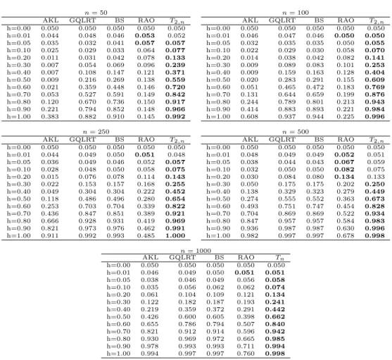
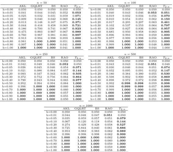
test. Tables 1 and 2 contain the empirical power function of each test. In these tables the bold face font is used to put in evidence the test statistics with the highest empirical power function EPow(h) for a given local alternative h >0. As mentioned before, the natural benchmark test statistics is the generalised quasi likelihood ratio test (GQLRT).
From this numerical analysis we can see several facts:
• the test statistic based on the AKL test statistics does not perform as the GQLR test despite they are related to the same divergence; the latter being sometimes better; • theT2,n seems to be (almost) uniformly more powerful in this experiment;
• all but RAO test seem to have a good behaviour when the alternative is sufficiently large; • for the CIR model, the RAO test does not perform well under the alternative hypothesis and this is probably because it requires very largeT which, in our case, is at mostT = 10. For the OU Gaussian case, the performance are better and in line from those presented in [21] for similar sample sizes.
Therefore, we can conclude that, despite all the test statistics share the same asymptotic prop-erties, the proposedTp,n seems to perform very well in the small sample case examined in the above Monte Carlo experiments, at least forp= 2.
6. Proofs
In order to prove the theorems appearing in the paper, we need some preliminary results. Let us start with the following lemmas.
Lemma 1. Fork≥1andtn
i−1≤t≤tni
(6.1) E0i−1[|Xt−Xi−1|k]≤Ck|t−tni−1|
k/2(1 +|X
i−1|)Ck. Iff : Θ×R→Ris of polynomial growth inxuniformly inθ then (6.2) E0i−1[f(θ, Xt)]≤Ct−tn i−1(1 +|Xi−1|) C, tn i−1≤t≤t n i.
Proof. See the proof of Lemma 6 in [23].
Lemma 2. Forl≥1 rl(∆n, Xi−1, θ) =Xi−1+ ∆nbi−1(α) +R(θ,∆2n, Xi−1) (6.3) E0i−1[(Xi−rl(∆n, Xi−1, θ))2] = ∆nci−1(β0) +R(θ,∆2n, Xi−1) (6.4) E0i−1[(Xi−rl(∆n, Xi−1, θ))3] =R(θ,∆2n, Xi−1) (6.5) E0i−1[(Xi−rl(∆n, Xi−1, θ))4] = 3∆2nc 2 i−1(β0) +R(θ,∆3n, Xi−1) (6.6) E0i−1[(Xi−rl(∆n, Xi−1, θ))5] =R(θ,∆3n, Xi−1) (6.7) E0i−1[(Xi−rl(∆n, Xi−1, θ))6] = 5·3∆3nc 3 i−1(β0) +R(θ,∆4n, Xi−1) (6.8) E0i−1[(Xi−rl(∆n, Xi−1, θ))7] =R(θ,∆4n, Xi−1) (6.9) E0i−1[(Xi−rl(∆n, Xi−1, θ))8] = 7·5·3∆4nc 4 i−1(β0) +R(θ,∆5n, Xi−1) (6.10)
Proof. The equalities from (6.3) to (6.6) represent the statement of Lemma 7 in [23]. By using the same approach adopted for the proof of the aforementioned lemma, we observe that from (6.3) to (6.6), the result (6.7) and (6.8) hold, if we are able to show that
E0i−1[(Xi−Xi−1)5] =R(θ,∆3n, Xi−1) (6.11) E0i−1[(Xi−Xi−1)6] = 5·3∆3nc 3 i−1(β0) +R(θ,∆4n, Xi−1) (6.12)
Table 1. Empirical power function EPow(h), for different sample sizesnand local alternativesh. The empirical power and theoretical power is 0.05. Data generating model: the 1-dimensional Ornstein-Uhlenbeck process.
n= 50 n= 100 AKL GQLRT BS RAO T2,n h=0.00 0.050 0.050 0.050 0.050 0.050 h=0.01 0.044 0.048 0.046 0.053 0.052 h=0.05 0.035 0.032 0.041 0.057 0.057 h=0.10 0.025 0.029 0.033 0.064 0.077 h=0.20 0.011 0.031 0.042 0.078 0.133 h=0.30 0.007 0.054 0.069 0.096 0.239 h=0.40 0.007 0.108 0.147 0.121 0.371 h=0.50 0.009 0.216 0.269 0.138 0.559 h=0.60 0.021 0.359 0.448 0.146 0.720 h=0.70 0.053 0.527 0.591 0.149 0.842 h=0.80 0.120 0.670 0.736 0.150 0.917 h=0.90 0.221 0.794 0.852 0.148 0.966 h=1.00 0.383 0.882 0.910 0.145 0.992 AKL GQLRT BS RAO T2,n h=0.00 0.050 0.050 0.050 0.050 0.050 h=0.01 0.046 0.047 0.046 0.050 0.050 h=0.05 0.032 0.035 0.035 0.050 0.055 h=0.10 0.022 0.029 0.030 0.058 0.070 h=0.20 0.014 0.038 0.042 0.082 0.141 h=0.30 0.009 0.089 0.083 0.101 0.253 h=0.40 0.009 0.159 0.163 0.128 0.404 h=0.50 0.020 0.283 0.291 0.155 0.609 h=0.60 0.051 0.465 0.472 0.183 0.769 h=0.70 0.131 0.644 0.659 0.199 0.876 h=0.80 0.244 0.789 0.801 0.213 0.943 h=0.90 0.414 0.883 0.893 0.221 0.984 h=1.00 0.608 0.937 0.944 0.225 0.996 n= 250 n= 500 AKL GQLRT BS RAO T2,n h=0.00 0.050 0.050 0.050 0.050 0.050 h=0.01 0.044 0.049 0.050 0.051 0.048 h=0.05 0.036 0.049 0.046 0.052 0.057 h=0.10 0.028 0.048 0.050 0.058 0.075 h=0.20 0.015 0.076 0.078 0.114 0.143 h=0.30 0.022 0.153 0.157 0.168 0.255 h=0.40 0.049 0.304 0.304 0.222 0.452 h=0.50 0.118 0.486 0.496 0.280 0.654 h=0.60 0.253 0.703 0.704 0.339 0.822 h=0.70 0.436 0.847 0.851 0.389 0.921 h=0.80 0.666 0.928 0.931 0.419 0.969 h=0.90 0.821 0.973 0.976 0.462 0.991 h=1.00 0.911 0.992 0.993 0.485 1.000 AKL GQLRT BS RAO T2,n h=0.00 0.050 0.050 0.050 0.050 0.050 h=0.01 0.048 0.049 0.049 0.052 0.051 h=0.05 0.038 0.044 0.043 0.067 0.059 h=0.10 0.032 0.050 0.050 0.082 0.075 h=0.20 0.030 0.084 0.080 0.134 0.133 h=0.30 0.050 0.175 0.175 0.202 0.250 h=0.40 0.138 0.329 0.323 0.279 0.449 h=0.50 0.274 0.555 0.552 0.363 0.673 h=0.60 0.493 0.751 0.747 0.454 0.828 h=0.70 0.704 0.869 0.869 0.522 0.934 h=0.80 0.847 0.957 0.957 0.584 0.983 h=0.90 0.936 0.987 0.987 0.630 0.996 h=1.00 0.982 0.997 0.997 0.678 0.998 n= 1000 AKL GQLRT BS RAO Tn h=0.00 0.050 0.050 0.050 0.050 0.050 h=0.01 0.046 0.049 0.050 0.051 0.051 h=0.05 0.038 0.046 0.049 0.056 0.058 h=0.10 0.035 0.056 0.062 0.062 0.074 h=0.20 0.061 0.104 0.109 0.121 0.134 h=0.30 0.122 0.182 0.187 0.193 0.241 h=0.40 0.219 0.359 0.372 0.291 0.442 h=0.50 0.426 0.600 0.605 0.398 0.662 h=0.60 0.655 0.786 0.794 0.507 0.840 h=0.70 0.821 0.912 0.914 0.596 0.942 h=0.80 0.930 0.969 0.972 0.665 0.985 h=0.90 0.978 0.993 0.993 0.711 0.994 h=1.00 0.994 0.997 0.997 0.760 0.998
We only prove (6.12), because (6.11) follows by means of similar arguments. By applying the Ito-Taylor formula (see Lemma 1, in [10]) to the function fx(y) = (y−x)6 we obtain
E0i−1[(Xi−Xi−1)6] =fXi−1(Xi−1) + ∆nL0fXi−1(Xi−1) +∆ 2 n 2 L 2 0fXi−1(Xi−1) + ∆3 n 3! L 3 0fXi−1(Xi−1) + Z ∆n 0 Z u1 0 Z u2 0 Z u3 0 E0i−1[L40fXi−1(Xti−n1+u4)]du1du2du3du4. By applying (6.2), we obtain Z ∆n 0 Z u1 0 Z u2 0 Z u3 0 E0i−1[L40fXi−1(Xtni−1+u4)]du1du2du3du4=R(θ,∆ 4 n, Xi−1).
Furthermore, by means of long and cumbersome calculations, we can show thatfx(x) =L0fx(x) =
L2
Table 2. Empirical power function EPow(h), for different sample sizes nand local alternativesh. The empirical power and theoretical power is 0.05. Data generating model: the 1-dimensional CIR process.
n= 50 n= 100 AKL GQLRT BS RAO T2,n h=0.00 0.050 0.050 0.050 0.050 0.050 h=0.01 0.041 0.044 0.045 0.052 0.053 h=0.05 0.025 0.032 0.031 0.059 0.071 h=0.10 0.009 0.040 0.042 0.068 0.145 h=0.20 0.013 0.148 0.167 0.075 0.371 h=0.30 0.044 0.416 0.458 0.069 0.721 h=0.40 0.186 0.700 0.741 0.067 0.923 h=0.50 0.475 0.883 0.907 0.067 0.989 h=0.60 0.760 0.967 0.981 0.061 0.997 h=0.70 0.913 0.994 0.998 0.059 1.000 h=0.80 0.981 1.000 1.000 0.051 1.000 h=0.90 0.997 1.000 1.000 0.041 1.000 h=1.00 1.000 1.000 1.000 0.041 1.000 AKL GQLRT BS RAO T2,n h=0.00 0.050 0.050 0.050 0.050 0.050 h=0.01 0.040 0.043 0.046 0.053 0.051 h=0.05 0.019 0.032 0.034 0.056 0.070 h=0.10 0.010 0.054 0.051 0.062 0.150 h=0.20 0.017 0.205 0.207 0.063 0.461 h=0.30 0.102 0.537 0.553 0.064 0.797 h=0.40 0.338 0.827 0.836 0.064 0.957 h=0.50 0.685 0.950 0.958 0.063 0.995 h=0.60 0.896 0.993 0.994 0.059 1.000 h=0.70 0.977 0.999 0.998 0.056 1.000 h=0.80 0.998 1.000 1.000 0.053 1.000 h=0.90 0.999 1.000 1.000 0.048 1.000 h=1.00 1.000 1.000 1.000 0.044 1.000 n= 250 n= 500 AKL GQLRT BS RAO T2,n h=0.00 0.050 0.050 0.050 0.050 0.050 h=0.01 0.042 0.049 0.046 0.052 0.050 h=0.05 0.026 0.045 0.046 0.054 0.071 h=0.10 0.021 0.086 0.084 0.057 0.144 h=0.20 0.093 0.347 0.342 0.062 0.505 h=0.30 0.372 0.752 0.756 0.064 0.864 h=0.40 0.790 0.943 0.944 0.065 0.977 h=0.50 0.952 0.994 0.994 0.064 1.000 h=0.60 0.996 1.000 1.000 0.060 1.000 h=0.70 1.000 1.000 1.000 0.060 1.000 h=0.80 1.000 1.000 1.000 0.057 1.000 h=0.90 1.000 1.000 1.000 0.055 1.000 h=1.00 1.000 1.000 1.000 0.050 1.000 AKL GQLRT BS RAO T2,n h=0.00 0.050 0.050 0.050 0.050 0.050 h=0.01 0.043 0.043 0.042 0.051 0.048 h=0.05 0.030 0.046 0.044 0.051 0.074 h=0.10 0.032 0.095 0.091 0.052 0.147 h=0.20 0.180 0.384 0.380 0.055 0.530 h=0.30 0.598 0.802 0.800 0.058 0.869 h=0.40 0.898 0.972 0.972 0.058 0.990 h=0.50 0.992 0.998 0.998 0.059 0.998 h=0.60 0.998 0.999 0.999 0.057 0.999 h=0.70 0.999 1.000 1.000 0.056 1.000 h=0.80 1.000 1.000 1.000 0.055 1.000 h=0.90 1.000 1.000 1.000 0.055 1.000 h=1.00 1.000 1.000 1.000 0.051 1.000 n= 1000 AKL GQLRT BS RAO T2,n h=0.00 0.050 0.050 0.050 0.050 0.050 h=0.01 0.044 0.048 0.047 0.051 0.050 h=0.05 0.035 0.059 0.057 0.051 0.079 h=0.10 0.067 0.120 0.118 0.054 0.144 h=0.20 0.274 0.429 0.428 0.058 0.527 h=0.30 0.725 0.844 0.840 0.061 0.886 h=0.40 0.953 0.983 0.983 0.062 0.989 h=0.50 0.996 0.998 0.998 0.062 0.999 h=0.60 1.000 1.000 1.000 0.062 1.000 h=0.70 1.000 1.000 1.000 0.060 1.000 h=0.80 1.000 1.000 1.000 0.059 1.000 h=0.90 1.000 1.000 1.000 0.059 1.000 h=1.00 1.000 1.000 1.000 0.058 1.000
Analogously to what done, from (6.3) to (6.8), the equalities (6.9) and (6.10) hold, if we are able to show that
E0i−1[(Xi−Xi−1)7] =R(θ,∆4n, Xi−1), (6.13) E0i−1[(Xi−Xi−1)8] = 7·5·3∆4nc 4 i−1(β0) +R(θ,∆5n, Xi−1). (6.14)
We only prove (6.14), because (6.13) follows by means of similar arguments. The application of the Ito-Taylor formula to the functionfx(y) = (y−x)8 yields
E0i−1[(Xi−Xi−1)8] =fXi−1(Xi−1) + ∆nL0fXi−1(Xi−1) + ∆2 n 2 L 2 0fXi−1(Xi−1) +∆ 3 n 3! L 3 0fXi−1(Xi−1) + ∆4 n 4! L 4 0fXi−1(Xi−1) + Z ∆n 0 Z u1 0 Z u2 0 Z u3 0 Z u4 0 E0i−1[L50fXi−1(Xtni−1+u5)]du1du2du3du4du5
By applying (6.2), we get Z ∆n 0 Z u1 0 Z u2 0 Z u3 0 Z u4 0 E0i−1[L50fXi−1(Xtni−1+u5)]du1du2du3du4du5=R(θ,∆ 5 n, Xi−1).
Furthermore, by means of long and cumbersome calculations, we can show thatfx(x) =L0fx(x) =
L2
0fx(x) =L30fx(x) = 0 whileL40fx(x) = 7·5·3·4!∆n4c4(β0, x).
Lemma 3 (Triangular arrays convegence). Let Un
i andU be random variables, with Uin being
Gn
i-measurable. The two following conditions imply
Pn i=1Uin P −→ n→∞U: n X i=1 E[Uin|Gin−1] P −→ n→∞U, n X i=1 E[(Uin)2|Gni−1] P −→ n→∞0
Proof. See the proof of Lemma 9 in [11].
Lemma 4. Let f : Θ×R→Rbe such thatf(θ, x)∈C↑1,1(Θ×R,R).Let us assumeA1−A6, if
∆n→0 andn∆n → ∞we have that 1 n n X i=1 fi−1(θ) P0 −→ n→∞ Z f(x, θ)π0(dx) uniformly in θ.
Proof. See the proof of Lemma 8 in [23].
Lemma 5. Let f : Θ×R→Rbe such thatf(θ, x)∈C↑1,1(Θ×R,R).Let us assumeA1−A6, if
∆n→0 andn∆n → ∞,asn→ ∞, we have that
1 n∆jn n X i=1 fi−1(θ)(Xi−rl(∆n, Xi−1, θ0))k P0 −→ n→∞ 0, j= 1, k= 1, R f(θ, x)c(β0, x)π0(dx), j= 1, k= 2, R f(θ, x)R(θ,1, x)π0(dx), j= 2, k= 3, 0, j= 1, k= 4, 3R f(θ, x)c2(β 0, x)π0(dx), j= 2, k= 4, uniformly in θ.
Proof. The cases j = 1, k = 1 and j = 1, k = 2 coincide with Lemma 9 and Lemma 10 in [23] and then we use the same approach to show that remaining convergences hold true.
By setting
ζin(θ) := 1
n∆2
n
fi−1(θ)(Xi−rl(∆n, Xi−1, θ0))3,
we prove that the convergence holds for allθ.By taking into account Lemma 2
E0i−1[ζin(θ)] = 1 n n X i=1 fi−1(θ)R(θ,1, Xi−1) P0 −→ n→∞ Z f(θ, x)R(θ,1, x)π0(dx), E0i−1[(ζin(θ))2] = 1 n2∆ n n X i=1 [5·3c3i−1(β0) +R(θ,1, Xi−1)] P0 −→ n→∞0.
Therefore by Lemma 3 we can conclude that
ζin(θ) P0
−→
n→∞ Z
for allθ.For the uniformity of the convergence we use the same arguments adopted in the proof of Lemma 8 in [23]. Hence, it is sufficient to prove the tightness of the sequence of random elements Yn(θ) := 1 n n X i=1 fi−1(θ)(Xi−rl(∆n, Xi−1, θ0))3 ∆2 n
taking values in the Banach spaceC(Θ) endowed with the sup-norm||·||∞.From the assumptions of lemma follows that supnE0[supθ∈Θ|∂θYn(θ)|] <∞ which implies the tightness of Yn(θ) for the criterion given by Theorem 16.5 in [19].
By setting
ζin(θ) := 1
n∆2
n
fi−1(θ)(Xi−rl(∆n, Xi−1, θ0))4,
we prove that the convergence holds for allθ.By taking into account Lemma 2 and Lemma 5
E0i−1[ζin(θ)] = 1 n n X i=1 fi−1(θ)[3c2i−1(β0) +R(θ,∆n, Xi−1)] P0 −→ n→∞3 Z f(θ, x)c2(β0, x)π0(dx), E0i−1[(ζin(θ)) 2 ] = 1 n2 n X i=1 [7·5·3c4i−1(β0) +R(θ,∆n, Xi−1)] P0 −→ n→∞0.
Therefore by Lemma 3 we get the pointwise convergence. For the uniformity of the convergence
we proceed as done above.
Before to proceed with the proofs of the main theorems of the paper, we introduce some useful quantities coinciding with (4.2)−(4.8) appearing in [23]. We can write down
lp,i(θ)−lp,i(θ0) =ϕi,1(θ, θ0) +ϕi,2(θ, θ0) +ϕi,3(θ, θ0) +ϕi,4(θ, θ0), (6.15) where ϕi,1(θ, θ0) := (Xi−rk0(∆n, Xi−1, θ0)) 2 2∆n ( 1 +Pk0 j=1∆ j ndj(θ, Xi−1) ci−1(β) −1 + Pk0 j=1∆ j ndj(θ0, Xi−1) ci−1(β0) ) , ϕi,2(θ, θ0) := (Xi−rk0(∆n, Xi−1, θ0))(rk0(∆n, Xi−1, θ0)−rk0(∆n, Xi−1, θ)) ∆nci−1(β) × 1 + k0 X j=1 ∆jndj(θ, Xi−1) , ϕi,3(θ, θ0) := (rk0(∆n, Xi−1, θ0)−rk0(∆n, Xi−1, θ)) 2 2∆nci−1(β) 1 + k0 X j=1 ∆jndj(θ, Xi−1) , ϕi,4(θ, θ0) := 1 2log ci−1(β) ci−1(β0) +1 2 k0 X j=1 ∆jn(ej(θ, Xi−1)−ej(θ0, Xi−1)). Furthermore ∂αhlp,i(θ) =η h i,1(θ) +η h i,2(θ), h= 1,2, ..., m1, (6.16) where ηhi,1(θ) :=−(∂αhrk0(∆n, Xi−1, θ))(Xi−rk0(∆n, Xi−1, θ)) n 1 +Pk0 j=1∆ j ndj(θ, Xi−1) o ∆nci−1(β) ,
ηi,h2(θ) := (Xi−rk0(∆n, Xi−1, θ)) 2 Pk0 j=1∆ j n∂αhdj(θ, Xi−1) 2∆nci−1(β) +1 2 k0 X j=1 ∆jn∂αhej(θ, Xi−1), and ∂βklp,i(θ) =ξ k i,1(θ) +ξi,k2(θ) +ξki,3(θ), k= 1,2, ..., m2, (6.17) where ξi,k1(θ) := (Xi−rk0(∆n, Xi−1, θ)) 2 2∆nci−1(β) k0 X j=1 ∆jn∂βkdj(θ, Xi−1) +1 2 k0 X j=1 ∆jn∂βkej(θ, Xi−1), ξi,k2(θ) :=−(Xi−rk0(∆n, Xi−1, θ)) 2∂ βkci−1(β) 2∆nc2i−1(β) 1 + k0 X j=1 ∆jndj(θ, Xi−1) +∂βkci−1(β) 2ci−1(β) , ξi,k3(θ) :=−(∂βkrk0(∆n, Xi−1, θ))(Xi−rk0(∆n, Xi−1, θ)) n 1 +Pk0 j=1∆ j ndj(θ, Xi−1) o ∆nci−1(β) .
From (6.15) it is possible to derive
∂α2 hαklp,i(θ) :=δ h,k i,1(θ) +δ h,k i,2(θ) +δ h,k i,3(θ) +δ h,k i,4(θ), h, k= 1,2, ..., m1, (6.18) where δi,h,k1(θ) := (Xi−rk0(∆n, Xi−1, θ0)) 2 2ci−1(β) {(∂α2 hαkd1)i−1(θ) +R(θ,∆n, Xi−1)}, δi,h,k2(θ) := (Xi−rk0(∆n, Xi−1, θ0)) ci−1(β) {−∂α2 hαkbi−1(α) +R(θ,∆n, Xi−1)}, δi,h,k3(θ) := 1 2∆n∂ 2 αhαke1(θ, Xi−1), δi,h,k4(θ) := ∆n ∂2 αhαkbi−1(α)(bi−1(α)−bi−1(α0)) +∂αhbi−1(α)∂αkbi−1(α) ci−1(β) +R(θ,∆n, Xi−1) , ∂2βhβklp,i(θ) :=ν h,k i,1(θ) +ν h,k i,2(θ) +ν h,k i,3(θ), h, k= 1,2, ..., m2, (6.19) where νi,h,k1(θ) := (Xi−rk0(∆n, Xi−1, θ0)) 2 2∆n {(∂β2 hβkc −1) i−1(β) +R(θ,∆n, Xi−1)}, νi,h,k2(θ) := 1 2(Xi−rk0(∆n, Xi−1, θ0))R(θ,1, Xi−1)), νi,h,k3(θ) := 1 2(∂ 2 βhβklogc)i−1(β) +R(θ,∆n, Xi−1)), and ∂α2 hβklp,i(θ) :=µi,1(θ) +µi,2(θ), h= 1,2, ..., m1, k= 1,2, ..., m2, (6.20) where µi,1(θ) := (Xi−rk0(∆n, Xi−1, θ0)) 2 2∆n R(θ,∆n, Xi−1), µi,2(θ) := (Xi−rk0(∆n, Xi−1, θ0)) ∆n R(θ,∆n, Xi−1) +R(θ,∆n, Xi−1).
Proof of Theorem 2. We observe that Dp,n(θ, θ0) = 1 n n X i=1 4 X k=1 (ϕi,k(θ, θ0))2+ 2 X j<k )ϕi,j(θ, θ0)ϕi,k(θ, θ0) .
UnderH0,from Lemma 4 and Lemma 5, we derive
1 n n X i=1 (ϕi,1(θ, θ0))2= 1 n n X i=1 " (Xi−rk0(∆n, Xi−1, θ0)) 4 4∆2 n 1 ci−1(β) − 1 ci−1(β0) +R(θ,∆n, Xi−1) 2# = 1 n n X i=1 " (Xi−rk0(∆n, Xi−1, θ0)) 4 4∆2 n 1 ci−1(β) − 1 ci−1(β0) 2# +oP0(1) P0 −→ n→∞ 3 4 Z c2(β0, x) 1 c(β, x)− 1 c(β0, x) 2 π0(dx) 1 n n X i=1 (ϕi,2(θ, θ0))2= 1 n n X i=1 (X i−rk0(∆n, Xi−1, θ0)) 2 c2 i−1(β0) [bi−1(α0)−bi−1(α)]2 +oP0(1) P0 −→ n→∞0 1 n n X i=1 (ϕi,3(θ, θ0))2= 1 n n X i=1 ∆2 n[bi−1(α0)−bi−1(α)]4 4c2 i−1(β) +oP0(1) P0 −→ n→∞0 1 n n X i=1 (ϕi,4(θ, θ0))2= 1 n n X i=1 1 4 log c i−1(β) ci−1(β0) 2 +oP0(1) P0 −→ n→∞ 1 4 Z log c(β, x) c(β0, x) 2 π0(dx) 1 n n X i=1 ϕi,1(θ, θ0)ϕi,4(θ, θ0) = 1 n n X i=1 (Xi−rk0(∆n, Xi−1, θ0)) 2 4∆n 1 ci−1(β) − 1 ci−1(β0) ×log c i−1(β) ci−1(β0) +oP0(1) P0 −→ n→∞ 1 4 Z c(β0, x) 1 c(β, x)− 1 c(β0, x) log c(β, x) c(β0, x) π0(dx) 1 n n X i=1 ϕi,1(θ, θ0)ϕi,j(θ, θ0) P0 −→ n→∞0, j= 2,3, 1 n n X i=1 ϕi,2(θ, θ0)ϕi,j(θ, θ0) P0 −→ n→∞0, j= 3,4, 1 n n X i=1 ϕi,3(θ, θ0)ϕi,4(θ, θ0) P0 −→ n→∞0,
Let Cp,n(θ, θ0) := 1 n∆n[∂ 2 αhαkTp,n(θ, θ0)]h=1,...,m1 k=1,...,m1 1 n√∆n[∂ 2 αhβkTp,n(θ, θ0)]h=1,...,m1 k=1,...,m2 1 n√∆n[∂ 2 αhβkTp,n(θ, θ0)]h=1,...,m1 k=1,...,m2 1 n[∂ 2 βhβkTp,n(θ, θ0)]h=1,...,m2 k=1,...,m2 (6.21) where ∂α2hαkTp,n(θ, θ0) = 2 n X i=1
∂αhlp,i(θ)∂αklp,i(θ) + [lp,i(θ)−lp,i(θ0)]∂ 2 αhαklp,i(θ) , (6.22) ∂β2 hβkTp,n(θ, θ0) = 2 n X i=1
∂βhlp,i(θ)∂βklp,i(θ) + [lp,i(θ)−lp,i(θ0)]∂ 2 βhβklp,i(θ) , (6.23) ∂α2 hβkTp,n(θ, θ0) = 2 n X i=1
∂αhlp,i(θ)∂βklp,i(θ) + [lp,i(θ)−lp,i(θ0)]∂ 2
αhβklp,i(θ) .
(6.24)
The following proposition concerning the asymptotic behavior of Cp,n(θ, θ0) plays a crucial
role in the proof of Theorem 3.
Proposition 1. Under H0, assumeA1−A6 and∆n →0, n∆n → ∞, asn→ ∞, the following
convergences hold Cp,n(θ0, θ0) P0 −→ n→∞2I(θ0) (6.25) and sup ||θ||≤εn ||Cp,n(θ0+θ, θ0)−Cp,n(θ0, θ0)|| P0 −→ n→∞0, εn→0. (6.26)
Proof of Proposition 1. We study the uniform convergence in probability ofCp,n(θ, θ0).Thus we
prove that uniformly inθ
(6.27) Cp,n(θ, θ0) P0 −→ n→∞2K(θ, θ0) := 2 K1(θ, θ0) +K2(θ, θ0) 0 0 K3(θ, θ0) +K4(θ, θ0) where K1(θ, θ0) := Z ∂ αhb(α, x)∂αkb(α, x) c2(β, x) c(β0, x)π0(dx), K2(θ, θ0) := 1 4 Z ∂α2hαkd1(x, θ) c(β 0, x) c(β, x) −1 3 c(β0, x) c(β, x) + log c(β, x) c(β0, x) −1 π0(dx) +1 2 Z ∂2 αhαkb(α, x)(b(α, x)−b(α0, x)) +∂αhb(α, x)∂αkb(α, x) c(β, x) × c(β 0, x) c(β, x) −1 + log c(β, x) c(β0, x) π0(dx) + Z −∂2 αhαkb(α, x) c(β, x) × 1 2 1 c(β0, x) − 1 c(β, x) R(θ,1, x) + c(β0, x) c2(β, x)(b(α, x)−b(α0, x)) π0(dx) K3(θ, θ0) := 1 2 Z c(β 0, x)∂βhc(β, x)∂βkc(β, x) c3(β, x) 3 2 c(β0, x) c(β, x) −1 +1 2 ∂βhc(β, x)∂βkc(β, x) c2(β, x) π0(dx), K4(θ, θ0) := 1 4 Z c(β0, x)∂β2hβklogc(β, x) 1 c(β, x)− 1 c(β0, x) π0(dx)
+1 4 Z log c(β, x) c(β0, x) c(β 0, x) c(β, x)∂ 2 βhβkc −1(β, x)π 0(dx) +1 4 Z log c(β, x) c(β0, x) ∂β2hβklogc(β, x)π0(dx).
Let us start with the analysis of the quantity n∆1
n∂ 2
αhαkTp,n(θ, θ0) given by (6.22) which can
be split in two terms. From (6.16) folllows that 1 n∆n n X i=1 ∂αhlp,i(θ)∂αklp,i(θ) = 1 n∆n n X i=1 (ηhi,1(θ) +ηi,h2(θ))(ηki,1(θ) +ηki,2(θ)) for each θ ∈ Θ. Since ∂αhrk0(∆n, Xi−1, θ) = ∆n∂αhbi−1(α) +R(θ,∆
2
n, Xi−1), by taking into
account Lemma 5, we get
1 n∆n n X i=1 ∂αhlp,i(θ)∂αklp,i(θ) = 1 n∆n n X i=1 ηi,h1(θ)ηi,k1(θ) +oP0(1) (6.28) = 1 n∆n n X i=1 ∂αhbi−1(α)∂αkbi−1(α) c2 i−1(β) (Xi−rk0(∆n, Xi−1, θ)) 2 +oP0(1) P0 −→ n→∞K1(θ, θ0)
uniformly in θ.Now, by resorting (6.15) and (6.18), we rewrite the second term appearing in (6.22) as follows 1 n∆n n X i=1
[lp,i(θ)−lp,i(θ0)]∂α2hαklp,i(θ) =
1 n∆n n X i=1 4 X l=1 4 X j=1 ϕi,l(θ, θ0)δi,jh,k(θ) .
By applying Lemma 1 and Lemma 5, the following convergence results hold 1 n∆n n X i=1 ϕi,1(θ, θ0)δi,h,k1(θ) P0 −→ n→∞ 3 4 Z ∂α2hαkd1(θ, x) c2(β0, x) c(β, x) 1 c(β, x)− 1 c(β0, x) π0(dx), 1 n∆n n X i=1 ϕi,1(θ, θ0)δi,h,k2(θ) P0 −→ n→∞ 1 2 Z −∂2 αhαkb(α, x) c(β, x) 1 c(β, x)− 1 c(β0, x) R(θ,1, x)π0(dx), 1 n∆n n X i=1 ϕi,1(θ, θ0)δ h,k i,3(θ) P0 −→ n→∞ 1 4 Z ∂α2 hαke1(θ, x) c(β 0, x) c(β, x) −1 π0(dx), 1 n∆n n X i=1 ϕi,1(θ, θ0)δ h,k i,4(θ) P0 −→ n→∞ 1 2 Z c(β 0, x) c(β, x) −1 ∂2 αhαkb(α, x)(b(α, x)−b(α0, x)) +∂αhb(α, x)∂αkb(α, x) c(β, x) π0(dx), 1 n∆n n X i=1 ϕi,2(θ, θ0)δ h,k i,2(θ) P0 −→ n→∞ Z c(β 0, x) c2(β, x)(−∂ 2 αhαkb(α, x))(b(α, x)−b(α0, x))π0(dx), 1 n∆n n X i=1 ϕi,4(θ, θ0)δ h,k i,1(θ) P0 −→ n→∞ 1 4 Z log c(β, x) c(β0, x) c(β 0, x) c(β, x)∂ 2 αhαkd1(θ, x)π0(dx), 1 n∆n n X i=1 ϕi,4(θ, θ0)δi,h,k3(θ) P0 −→ n→∞ 1 4 Z ∂α2hαke1(θ, x) log c(β, x) c(β0, x) π0(dx),
1 n∆n n X i=1 ϕi,4(θ, θ0)δh,ki,4(θ) P0 −→ n→∞ 1 2 Z log c(β, x) c(β0, x) ∂2 αhαkb(α, x)(b(α, x)−b(α0, x)) +∂αkb(α, x)∂αhb(α, x) c(β, x) π0(dx), 1 n∆n n X i=1 ϕi,2(θ, θ0)δh,ki,j(θ) P0 −→ n→∞0, j= 1,3,4, 1 n∆n n X i=1 ϕi,3(θ, θ0)δh,ki,j(θ) P0 −→ n→∞0, j= 1,2,3,4, 1 n∆n n X i=1 ϕi,4(θ, θ0)δh,ki,2(θ) P0 −→ n→∞0,
uniformly inθ.Finally, since d1(θ, x) =−e1(θ, x),we get
1
n∆n n
X
i=1
[lp,i(θ)−lp,i(θ0)]∂α2hαklp,i(θ)
P0
−→
n→∞K2(θ, θ0).
(6.29)
uniformly inθ.Hence, by (6.28) and (6.29), we immediately derive 1 n∆n ∂α2 hαkTp,n(θ, θ0) P0 −→ n→∞2(K1(θ, θ0) +K2(θ, θ0)) (6.30) uniformly inθ.
Now, we consider the elements of the matrix Cn,p(θ, θ0) given by (6.23). First, we study the
convergence probability of 1 n n X i=1 ∂βhlp,i(θ)∂βklp,i(θ) = 1 n n X i=1 (ξi,h1(θ) +ξhi,2(θ) +ξi,h3(θ))(ξki,1(θ) +ξi,k2(θ) +ξi,k3(θ)). Since∂βhrk0(∆n, Xi−1, θ) =R(θ,∆ 2
n, Xi−1),from Lemma 5 and Lemma 1 we derive
1 n n X i=1 ∂βhlp,i(θ)∂βklp,i(θ) = 1 n n X i=1 ξi,h2(θ)ξi,k2(θ) +oP0(1) (6.31) = 1 n n X i=1 ∂βhci−1(β)∂βkci−1(β) 4∆2 nc4i−1(β) (Xi−rk0(∆n, Xi−1, θ)) 4 +1 n n X i=1 ∂βhci−1(β)∂βkci−1(β) 2∆nc3i−1(β) (Xi−rk0(∆n, Xi−1, θ)) 2 +1 n n X i=1 ∂βhci−1(β)∂βkci−1(β) 4c2 i−1(β) +oP0(1) P0 −→ n→∞K3(θ, θ0)
uniformly in θ. Now, by resorting (6.15) and (6.17), we rewrite the second term appearing in (6.23) as follows 1 n n X i=1
[lp,i(θ)−lp,i(θ0)]∂2βhβklp,i(θ) =
1 n n X i=1 4 X k=1 3 X j=1 ϕi,k(θ, θ0)νi,jh,k(θ) .
By taking into account again Lemma 1 and Lemma 5, the following results yield 1 n n X i=1 ϕi,1(θ, θ0)νi,3(θ) P0 −→ n→∞ 1 4 Z c(β0, x)∂β2hβklogc(β, x) 1 c(β, x)− 1 c(β0, x) π0(dx) 1 n n X i=1 ϕi,4(θ, θ0)νi,1(θ) P0 −→ n→∞ 1 4 Z log c(β, x) c(β0, x) c(β 0, x) c(β, x)∂ 2 βhβkc −1 (β, x)π0(dx) 1 n n X i=1 ϕi,4(θ, θ0)νi,3(θ) P0 −→ n→∞ 1 4 Z log c(β, x) c(β0, x) ∂β2 hβklogc(β, x)π0(dx) 1 n n X i=1 ϕi,1(θ, θ0)νi,j(θ) P0 −→ n→∞0, j= 1,2, 1 n n X i=1 ϕi,k(θ, θ0)νi,j(θ) P0 −→ n→∞0, k, j= 1,2,3, 1 n n X i=1 ϕi,4(θ, θ0)νi,2(θ) P0 −→ n→∞0, uniformly inθ.Finally 1 n n X i=1
[lp,i(θ)−lp,i(θ0)]∂β2hβklp,i(θ)
P0
−→
n→∞K4(θ, θ0)
(6.32)
uniformly inθ.Therefore, by (6.31) and (6.32), we get 1 n∂ 2 βhβkTp,n(θ, θ0) P0 −→ n→∞2(K3(θ, θ0) +K4(θ, θ0)) (6.33) uniformly inθ.
Recalling the expressions (6.16), (6.17), (6.20) and (6.15), by means of similar arguments adopted above, it is not hard to prove that
1 n√∆n n X i=1 ∂αhlp,i(θ)∂βklp,i(θ) P0 −→ n→∞0 and 1 n√∆n n X i=1
[lp,i(θ)−lp,i(θ0)]∂α2hβklp,i(θ)
P0
−→
n→∞0
uniformly inθ.This implies that 1 n√∆n ∂α2 hβkTp,n(θ, θ0) P0 −→ n→∞0 (6.34) uniformly inθ.
In conclusion the results (6.30), (6.33) and (6.34) lead to the convergence (6.27). Moreover, immediately (6.27) implies (6.25) sinceK(θ0, θ0) =I(θ0). From the inequality
sup ||θ||≤εn ||Cp,n(θ0+θ, θ0)−Cp,n(θ0, θ0)|| ≤ sup ||θ||≤εn ||Cp,n(θ0+θ, θ0)−2K(θ0+θ, θ0)||+ sup ||θ||≤εn ||2K(θ0+θ, θ0)−2I(θ0)|| +||2I(θ0)−Cp,n(θ0, θ0)||
follows (6.26). Indeed, (6.25) leads to ||2I(θ0)−Cp,n(θ0, θ0)|| −→
n→∞0, εn → 0, while the term
sup||θ||≤ε
n||Cp,n(θ0+θ, θ0)−2K(θ0+θ, θ0)||
P0
−→
n→∞0, εn →0,by the uniformity of the convergence
(i.e. by the result (6.27)). Furthermore, sup||θ||≤εn||K(θ0+θ, θ0)−I(θ0)||
P0
−→
n→∞0, εn →0,because
the assumptionsA3 andA5,imply thatK(θ, θ0) is a continuous function with respect to θ.
Now, we are able to prove Theorem 3.
Proof of Theorem 3. We adopt classical arguments. By Taylor’s formula, we have that
Tp,n(ˆθp,n, θ0) =Tp,n(θ0, θ0) +n∂θTp,n(θ0, θ0)(ˆθp,n−θ0) (6.35) +1 2((ˆθn−θ0)ϕ(n) −1/2)0Λ p,n(ˆθp,n, θ0))ϕ(n)−1/2(ˆθp,n−θ0) = 1 2((ˆθn−θ0)ϕ(n) −1/2)0Λ p,n(ˆθp,n, θ0)ϕ(n)−1/2(ˆθn−θ0)
where in the last step we denoted by Λp,n(ˆθp,n, θ0) :=ϕ(n)1/2 Z 1 0 (1−u)∂θ2Tp,n(θ0+u(ˆθp,n−θ0), θ0)duϕ(n)1/2 = Z 1 0 (1−u)[Cp,n(θ0+u(ˆθp,n−θ0), θ0)−Cp,n(θ0, θ0)]du+ 1 2Cp,n(θ0, θ0). Proposition 1 implies (6.36) Λp,n(ˆθp,n, θ0) P0 −→ n→∞2I(θ0).
By taking into account (6.35), (3.16) and (6.36), Slutsky’s theorem allows to conclude the proof.
Proof of Theorem 4. UnderH1,n we have that (see Lemma 2 in [21])
ϕ(n)−1/2(ˆθp,n−(θ0+ϕ(n)h))
d
−→
n→∞N(0, I(θ0) −1).
Therefore, under the hypothesisH1,n
ϕ(n)−1/2(ˆθp,n−θ0) =ϕ(n)−1/2(ˆθp,n−θ) +h d −→ n→∞N(h, I(θ0) −1) and Cp,n(ˆθp,n, θ0) Pθ −→ n→∞2I(θ0) (underH1,n).
Hence, from (6.35) we obtain the result (4.7).
Conflict of interest
On behalf of all authors, the corresponding author states that there is no conflict of interest.
References
[1] A¨ıt-Sahalia, Y. (1996) Testing continuous-time models of the spot interest rate,Review of Financial Studies, 70, 385–426.
[2] A¨ıt-Sahalia, Y. (2002). Maximum-likelihood estimation of discretely-sampled diffusions: A closed-form ap-proximation approach,Econometrica,70, 223–262.
[3] A¨ıt-Sahalia, Y. (2008) Closed-form likelihood expansions for multivariate diffusions,Annals of Statistics36, 906-937.
[4] Balakrishnan, V., Sanghvi, L. D. (1968) Distance between populations on the basis of attribute data, Biomet-rica,24, 859-865.
[5] Bibby, B.M., Sørensen, M. (1995) Martingale estimating functions for discretely observed diffusion processes,
Bernoulli,1, 17-39.
[6] De Gregorio, A., Iacus, S.M. (2008) Least squares volatility change point estimation for partially observed diffusion processes,Comm. Statist. Theory Methods,37, 2342-2357.
[7] De Gregorio, A., Iacus, S.M. (2010) Clustering of discretely observed diffusion processes, Computational Statistics and Data Analysis,54, 598-606.
[8] De Gregorio, A., Iacus, S.M. (2012) Adaptive LASSO-type estimation for multivariate diffusion processes,
Econometric Theory,28, 838-860.
[9] De Gregorio, A., Iacus, S.M. (2013) On a family of test statistics for discretely observed diffusion processes,
Journal of Multivariate Analysis,122, 292-316.
[10] Florens-Zmirou, D. (1989) Approximate discrete-time schemes for statistics of diffusion processes,Statistics, 20, 547-557.
[11] Genon-Catalot, V., Jacod, J. (1993) On the estimation of the diffusion coefficient for multidimensional diffusion processes,Ann. Inst. Henri Poincar´e,29, 119–151.
[12] Gobet, E. (2002) LAN property for ergodic diffusions with discrete observations,Ann. I. H. Poincar´e – PR, 38, 711-737.
[13] Iacus, S.M. (2008)Simulation and Inference for Stochastic Differential Equations: with R examples, Springer Series in Statistics, Springer NY.
[14] Iacus, S.M. (2011)Option pricing and estimation of financial models with R, John Wiley & Sons, Ltd. [15] Iacus, S.M., Uchida, M., Yoshida, N. (2009) Parametric estimation for partially hidden diffusion processes
sampled at discrete times,Stochastic Processes and their Applications,119, 1580-1600.
[16] Iacus, S.M., Yoshida, N. (2012) Estimation for the change point of volatility in a stochastic differential equation,Stochastic Processes and their Applications,122, 1068-1092.
[17] Iacus, S.M., Yoshida, N. (2017)Simulation and Inference for Stochastic Processes with YUIMA, Springer Series in Statistics, Springer NY.
[18] Jacod, J. (2006) Parametric inference for discretely observed non-ergodic diffusions,Bernoulli,12, 383-401. [19] Kallenberg, O. (2001)Foundations of Modern Probability, Springer-Verlag, London.
[20] Kamatani, K., Uchida, M. (2015) Hybrid multi-step estimators for stochastic differential equations based on sampled data,Statistical Inference for Stochastic Processes,18, 177-204.
[21] Kitagawa, H., Uchida, M. (2014) Adaptive test statistics for ergodic diffusion processes sampled at discrete times,Journal of Statistical Planning and Inference,150, 84-110.
[22] Kessler, M., (1995) Estimation des parametres d’une diffusion par des contrastes corrig´es,C. R. Acad. Sci. Paris Ser. I Math.,320, 359-362. Math. 320 (1995) 359–362.
[23] Kessler, M. (1997) Estimation of an ergodic diffusion from discrete observations,Scand. J. Stat.,24, 211–229. [24] Kessler, M., Sørensen, M. (1999) Estimating equations based on eigenfunctions for a discretely observed
diffusion process,Bernoulli,5, 299-314.
[25] Kutoyants, Yu. A. (2004)Statistical Inference for Ergodic Diffusion Processes, Springer-Verlag, London. [26] Li, C. (2013) Maximum-likelihood estimation for diffusion processes via closed-form density expansions,
Annals of Statistics,41, 1350-1380.
[27] Morales, D., Pardo, L., Vajda, I. (1997) Some New Statistics for Testing Hypotheses in Parametric Models,
Journal of Multivariate Analysis,67, 137-168.
[28] Pardo, L. (2006)Statistical Inference Based on Divergence Measures, Chapman & Hall/CRC, London. [29] Phillips, P.C.B., Yu, J. (2009) A two-stage realized volatility approach to estimation of diffusion processes
with discrete data,Journal of Econometrics,150. 139-150.
[30] Uchida, M., Yoshida, N. (2012) Adaptive estimation of an ergodic diffusion process based on sampled data,
Stochastic Process. Appl.,17, 181-219.
[31] Uchida, M., Yoshida, N. (2014) Adaptive Bayes type estimators of ergodic diffusion processes from discrete observations,Statistical Inference for Stochastic Processes,122, 2885-2924.
[32] Van der Vaart, A.W. (1998)Asymptotic Statistics, Cambridge University press,
[33] Yoshida, N. (1992) Estimation for diffusion processes from discrete observation,J. Multivariate Anal.,41, 220-242.
[34] Yoshida, N. (2011) Polynomial type large deviation inequality and its applications,Ann. Inst. Stat. Mat., 63, 431-479.
Department of Statistical Sciences, “Sapienza” University of Rome, P.le Aldo Moro, 5 - 00185, Rome, Italy
Dipartimento di Economia, Management e Metodi Quantitativi, Via Conservatorio 7, 20122 - Milan, Italy
E-mail address:[email protected] E-mail address:[email protected]