Georgia State University
Georgia State University
ScholarWorks @ Georgia State University
ScholarWorks @ Georgia State University
EBCS Articles
Evidence-Based Cybersecurity Research Group
2018
Continuous Restricted Boltzmann Machines
Continuous Restricted Boltzmann Machines
Robert W. Harrison
Georgia State University
Follow this and additional works at: https://scholarworks.gsu.edu/ebcs_articles
Part of the Computer Sciences Commons
Recommended Citation
Recommended Citation
Harrison, Robert W. 2018. Continuous Restricted Boltzmann Machines. Wireless Networks. https://doi.org/10.1007/s11276-018-01903-6.
This Article is brought to you for free and open access by the Evidence-Based Cybersecurity Research Group at ScholarWorks @ Georgia State University. It has been accepted for inclusion in EBCS Articles by an authorized administrator of ScholarWorks @ Georgia State University. For more information, please contact
Continuous Restricted Boltzmann Machines
Robert W. Harrison1
Department of Computer Science, Georgia State University, Atlanta Georgia USA.
Abstract. Restricted Boltzmann machines are a generative neural net-work. They summarize their input data to build a probabilistic model that can then be used to reconstruct missing data or to classify new data. Unlike discrete Boltzmann machines, where the data are mapped to the space of integers or bitstrings, continuous Boltzmann machines di-rectly use floating point numbers and therefore represent the data with higher fidelity. The primary limitation in using Boltzmann machines for big-data problems is the efficiency of the training algorithm. This pa-per describes an efficient deterministic algorithm for training continuous machines.
Keywords: Deep learning, Data mining, Energy-based learning, Restricted Boltz-mann machines
1
Introduction
Restricted Boltzmann machines (RBMs) [12] develop a energy-based model of the data presented to them. Since RBMs learn to recognize the data they have seen [6, 11, 4], they are well-suited to extracting and reconstructing consistent patterns in the data. In a very real sense they straddle the divide between unsu-pervised and suunsu-pervised learning algorithms. Because they are regenerative, they are also a prototype of deep learning, and can serve as an ”adapter” between real data and a more abstract representation suitable for other machine learn-ing approaches. For a recent review of the manifold versions of RBMs that are used, see [3] . RBMs are inherently probabilistic recognizers and can interface effectively with fuzzy representations of uncertainty. We developed an efficient training algorithm for fuzzy discrete RBMs and this algorithm builds on that work[8, 7].
The classic or discrete RBM (dRBM) restricts the input and output data to integer values or bitstrings. Real valued data typically are mapped to unique bit-strings. This results in a loss of fidelity in the reconstruction because only the bitstring can be reproduced. The encoding or mapping is also problem-dependent and the use of a sub-optimal encoding will result in sub-optimal training, classification, and reconstruction.
Continuous RBMs (cRBM) replace discrete valued spins with continuous val-ues. The problem of training an RBM shifts from enumerating independent spins to estimating the continuous values of the hidden variables. Chen and Murray
introduced the first practical cRBM in 2003 [4]. This paper introduces a deter-ministic training algorithm for the cRBM. It shows that using least square error estimates for the hidden variables is computationally tractable and gives excel-lent results. The paper demonstrates that the classification and reconstruction accuracy of a cRBM is competitive with other machine learning methods.
2
Algorithm and Implementation
The general algorithm for a RBM trains or optimizes a potential against data [10]. A full discrete Boltzmann machine uses a spin-lattice construct of hidden variables to enumerate states and seeks to find an energy minimum over that lattice given an observed set of data. Since the number of possible states of the spin-lattice is exponential, simplifications such as the RBM have been devel-oped. An RBM uses a layer of independent hidden variables and thus the number of possible states is a linear function of the number of hidden variables. Con-ventional RBMs use an iterative stochastic optimization algorithm, contrastive divergence, for training. Replacing the stochastic algorithm with an analytic approximation results in considerable simplifications to the algorithm[8].
2.1 Algorithm
The specific steps in the algorithm are given in 1. The formal background of the algorithm for a continuous Boltzmann machine starts from the definition of the potential energy: U =X i X j ViWi,jHj=VtW U (1)
Where Vi are the observed data, Wi,j are the weights and Hj are the hidden values. A bias could be added to both the observed data and hidden values. However, since the bias is colinear with the data and hidden values we set it to a constant of zero. Adding a bias would replace Hj with (Hj−bhj) and Vi with (Vi−bvi) where bv and bh are visible and hidden layer bias values. The free energy is by definition and as an analogy the the Helmholtz free energy in statistical mechanics: F= −1 β ln( X samples e−βU) (2)
The partition functionZis defined asP
samplese
−βU, and the probability of any one state is given by e−ZβU. Taking the derivative of F yields the probability:
dF dUi
= 1
Ze
−βUi =P(Ui) (3)
thus by the chain rule, the derivative of F with respect to a parameter p is:
dF dp = X i df dUi dUi dp = X i Pi dUi dp =< dUi dp > (4)
where<>denotes expected value. Maximizing U to train and minimizingF to prevent over-training results in the total derivative dUdp −dF
dp or dU
dp−< dU
dp >. Taking the derivative ofU−F with respect to Wi,j results in:
X i X j ViHj−< X i X j ViHj >=VtH−< VtH > (5)
which encapsulated Hebbian learning in the correlation between V and H[9, 17, 11].
Two major difficulties arise in the use of equation 5. The first is the evaluation of the expected value term and the second is the evaluation ofHj. Contrastive divergence [10, 12, 18] finds a numerical approximation for < dWdU >. Previous work [8, 7] describes an analytic approach to training the discrete RBM that converges to the same results and is much faster than contrastive divergence. Moving from the discrete model to a continuous model requires shifting from a sum over two states (spins of±1) to an integral over the changes in potential. Numerical approximations readily converge for this integral and we use:
< dU
dW >=dW
3e−βU(W+dW)
e−βU(W−dW)+e−βU(W)+e−βU(W+dW) (6)
wheredWi,j isViHj.
EvaluatingHj is more difficult. Naively using the gradient dHdU j =
P iViWi,j to estimateHtends to lose information and converge to a uniform set of weights. Forming the least squares estimate that matches H and V given W gives far better results. The rows of W form a basis set for expanding V in the least squares algorithm. dU dV = X j Wi,jHj (7) Vcalc=δ dU dV (8)
minimizeQ= (V −Vcalc)2 overH (9)
dQ
dH =−2(V −Vcalc) dVcalc
dH = 0 at the minimum. (10)
This leads to the following Matrix equation: (X i Wi,jVi) = ( X i Wi,jWi,k)(Hj) =WtW H=N H (11)
Where N is the normal equation of the system. N is a symmetric, diagonally dominant, matrix. During training, N may be ill-conditioned, so as a practical matter, it is regularized by adding λI. In this paper λ= 1 and the magnitude of the elements of N is typically about 100-1000. The code used in this paper solved the normal equation with Gaussian elimination every time H was gen-erated. Production code would save time by either storing N−1 or using a LU
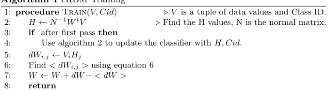
Algorithm 1cRBM Training
1: procedureTrain(V, Cid) . V is a tuple of data values and Class ID. 2: H ←N−1WtV .Find the H values, N is the normal matrix. 3: if after first passthen
4: Use algorithm 2 to update the classifier withH, Cid. 5: dWi,j←ViHj
6: Find< dWi,j>using equation 6
7: W ←W+dW−< dW >
8: return
decomposition. This approach is a version of the Levenberg-Marquardt algorithm [16] applied to training and other approaches to accelerating the calculation (as in [14]) can be evaluated in future work.
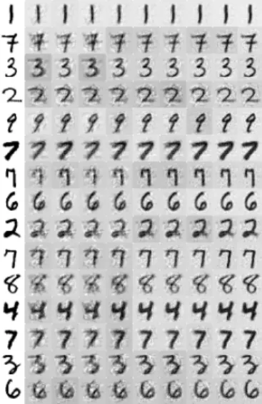
Figure 1 shows the quality of reconstructions when applied to the MNIST data set.
2.2 Classification Algorithm
The values of the energy and the quality of the reconstruction are poor predictors of class membership with cRBMs. In essence, the reconstruction algorithm is too good for the errors to be a reliable indicator of class membership. Since the rows ofW are a basis set andH is the expansion of the data in that basis, the values of H are useful for classifying data. Since the rank of W is often lower than the number of features or the number of features times the number of classes, the values of H are a compressed representation of the data. Algorithm 2 was used to train the classifier. It selects points that are along the boundary between classes.
Algorithm 2Classifier Training
1: procedureTrain(H, Cid) . H, Cidis a tuple of Hidden layer values and Class ID.
2: R←closest point toH
3: Rs←closest point toH with Class == Cid
4: if |R|<|Rs|then .Not correctly predicted
5: Rs←H .ReplaceRs, CidwithH, Cid
6: else
7: already correct, leave intact. 8: return
3
Results
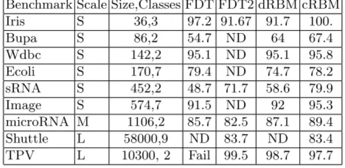
Table 3 shows the performance of the cRBM on a range of problems taken from the UCI repository [15], and used in our previous work on the Fuzzy Decision
Benchmark Scale Size,Classes FDT FDT2 dRBM cRBM Iris S 36,3 97.2 91.67 91.7 100. Bupa S 86,2 54.7 ND 64 67.4 Wdbc S 142,2 95.1 ND 95.1 95.8 Ecoli S 170,7 79.4 ND 74.7 78.2 sRNA S 452,2 48.7 71.7 58.6 79.9 Image S 574,7 91.5 ND 92 95.3 microRNA M 1106,2 85.7 82.5 87.1 89.4 Shuttle L 58000,9 ND 83.7 ND 83.4 TPV L 10300, 2 Fail 99.5 98.7 97.7
Table 1.Benchmark Results. The performance of this cRBM was tested against stan-dard datasets.
Trees (FDT) [1, 2, 5] and dRBMs [8]. The best results for the dRBMs, after optimizing the encoding to discrete bitstrings, were included in the table. The prescribed training and test sets were used for all of the UCI datasets and the others were evaluated with five-fold cross validation with the mean accuracy reported. The new algorithm consistently out-performs the older ones. While not shown, the PPV, recall and F-scores are consistent with the level of accuracy in the results. The correlation between the reconstructed data, determined by equation 8 and the input data is> 0.99 for most of the data sets. (TPV is an exception where it is only>0.9).
Benchmarking the approach against HIVpr drug resistance data taken from Yu et al[20] and shown in table 2 demonstrates that it can handle relatively large datasets. The approach in [20] maps drug resistant mutations onto the molecular structure and uses Delaunay triangulation to reduce it to a 210 long feature vector. The Yu paper uses compressed encoding as well as SVM and ANN so it is a relevant comparison. The average values for 5-fold cross validation and standard errors are reported for this data.
Inhibitor Yu Accuracy Accuracy PPV Recall F idv 96.1 94.8±0.1 94.1±0.9 92.9±1.0 93.4±0.2 lpv 95.9 95.1±0.3 95.5±0.3 93.0±0.8 94.2±0.4 sqv 95.0 93.6±0.3 95.8±0.2 91.9±0.8 93.8±0.4 tpv 96.1 97.7±0.2 98.2±0.2 97.8±0.1 98.0±0.2
Table 2.Results on benchmark HIVpr data. The same data that were used in [20] were used for this test. There are 210 features and between 10000 and 17000 data points. These are the results from five-fold cross validation using 10 hidden layers.
The MNIST character recognition data set consists of 60,000 scanned and centered handwritten digits for training and 10,000 digits for testing[13, 19]. Figure 1 shows the quality of the reconstruction with a cRBM as a function of the number of hidden layers. The cRBM achieved accuracies of between 94.6%
and 95.4%. Fuzzy RBMs[8] reached accuracies between 94.6% and 95.7% when trained with 1000 hidden units (either divided into ten 100-deep classifiers or treated as on large one of 1000 layers). This accuracy is comparable to a 2-layer NN[13]. cRBMs use a significantly smaller number of hidden layers to achieve similar accuracy to the earlier work (table 3 shows the results for the cRBM using 40 layers). Note that the 40 layers used in the cRBM is much smaller than the 1000 layers used in the dRBM. Surprisingly the classification accuracy degrades as the number of hidden layers rises, while the quality of the reconstruction (figure 1) improves. This strongly suggests that improving the quality of the classification algorithm used on the hidden layers would be fruitful.
Number of hidden layers Accuracy
40 95.4
80 95.2
100 94.6 200 91.8
Table 3.Results on the MNIST dataset. The accuracy is shown as a function of the number of hidden layers.
Fig. 1. A sample of digits from the MNIST data set is shown for the original data followed by reconstructions with 40, 60, 80, 100, 120, 140, 160, 180, and 200 hidden layers. The cRBM was trained on the standard training set and the reconstructions are from the testing set.
The code was written in C++ and complied with the GNU compiler. Other than the MNIST benchmark, all the calculations were performed on a small laptop computer (1.6GHz lenovo n22, using Ubuntu under windows 10) in a matter of minutes. The exact times depend on training parameters, but the cited examples from table 3 took 205 seconds for the microRNA set with 50 hidden layers and 60 seconds for the shutle set with 10 hidden layers. The MNIST data took about an hour of CPU time per point on a 1.6GHz linux workstation. Ten training epochs were used in all the examples.
4
Conclusion
This paper demonstrated an effective algorithm for classification and reconstruc-tion using a continuous RBM. The accuracy of the predicreconstruc-tions was competitive with other methods when validated either against standard test sets or by 5-fold cross validation. Several areas for improvement remain. Namely, the naive 1-NN classification algorithm should be replaced with a more accurate one, and the mechanics of the least square estimation of H could be implemented in a more effective manner. There is no reason that the algorithm cannot be implemented on a GPU with significant performance enhancement.
Acknowledgements
The research was supported in part by the National Institutes of Health grant GM062920.
References
1. Abu-halaweh, N.M., Harrison, R.W.: Practical fuzzy decision trees. In: 2009 IEEE Symposium on Computational Intelligence and Data Mining. pp. 211–216 (March 2009)
2. Abu-halaweh, N.M., Harrison, R.W.: Identifying essential features for the classi-fication of real and pseudo microRNAs precursors using fuzzy decision trees. In: 2010 IEEE Symposium on Computational Intelligence in Bioinformatics and Com-putational Biology. pp. 1–7 (May 2010)
3. Bengio, Y., Courville, A., Vincent, P.: Representation learning: A review and new perspectives. IEEE Transactions on Pattern Analysis and Machine Intelligence 35(8), 1798–1828 (Aug 2013)
4. Chen, H., Murray, A.F.: Continuous restricted boltzmann machine with an imple-mentable training algorithm. IEE Proceedings - Vision, Image and Signal Process-ing 150(3), 153–158 (June 2003)
5. Durham, E.E.A., Yu, X., Harrison, R.W.: FDT 2.0: Improving scalability of the fuzzy decision tree induction tool - integrating database storage. In: 2014 IEEE Symposium on Computational Intelligence in Healthcare and e-health (CICARE). pp. 187–190 (Dec 2014)
6. Fischer, A., Igel, C.: Training restricted boltzmann machines: An introduction. Pattern Recognition 47(1), 25–39 (2014)
7. Harrison, R., McDermott, M., Umoja, C.: Recognizing protein secondary structures with neural networks. In: Database and Expert Systems Applications (DEXA), 2017 28th International Workshop on. pp. 62–68. IEEE (2017)
8. Harrison, R.W., Freas, C.: Fuzzy restricted boltzmann machines. In: North Amer-ican Fuzzy Information Processing Society Annual Conference. pp. 392–398. Springer, Cham (2017)
9. Hebb, D.O.: Organization of behavior. Wiley, New York (1949)
10. Hinton, G.E.: Training Products of Experts by Minimizing Contrastive Divergence. Neural Computation 14(8), 1771–1800 (Aug 2002)
11. Hinton, G.: UTML TR 2010003 A Practical Guide to Training Restricted Boltz-mann Machines (2010), http://www.cs.toronto.edu/˜hinton/absps/guideTR.pdf 12. Hinton, G.E.: Training products of experts by minimizing contrastive divergence.
Neural Computation 14(8), 1771 – 1800 (2002)
13. LeCunn, Y., Cortes, C., and Burges, C.J.C.: (2017), http://yann.lecun.com/exdb/mnist/
14. Lera, G., Pinzolas, M.: Neighborhood based levenberg-marquardt algorithm for neural network training. IEEE Transactions on Neural Networks 13(5), 1200–1203 (Sep 2002)
15. Lichman, M.: UCI machine learning repository (2013), http://archive.ics.uci.edu/ml
16. Marquardt, D.: An algorithm for least-squares estimation of nonlinear parameters. Journal of the Society for Industrial and Applied Mathematics 11(2), 431–441 (1963), https://doi.org/10.1137/0111030
17. McMillen, T., Simen, P., Behseta, S.: Hebbian learning in linearnon-linear networks with tuning curves leads to near-optimal, multi-alternative decision making. Neural Networks 24(5), 417 – 426 (2011), http://www.sciencedirect.com/science/article/pii/S0893608011000293
18. R. Salakhutdinov, G.E.H.: An Efficient Learning Procedure for Deep Boltzmann Machines. Neural Computation 24(8), 1967 – 2006 (2012)
19. Y. Lecun and L. Bottou and Y. Bengio and P. Haffner: Gradient-based learning applied to document recognition. Proceedings of the IEEE 86(11), 2278–2324 (Nov 1998)
20. Yu, X., Weber, I., Harrison, R.: Sparse representation for hiv-1 protease drug re-sistance prediction. In: Proceedings of the 2013 SIAM International Conference on Data Mining. pp. 342–349. SIAM (2013)