Localized Realized Volatility Modelling

Localized Realized

Volatility Modelling

Ying Chen*

Wolfgang Karl Härdle**

Uta Pigorsch***

SFB 649 Discussion Paper 2009-003

S

FB

6

4

9

E

C

O

N

O

M

I

C

R

I

S

K

B

E

R

L

I

N

*National University of Singapore **Humboldt-Universität zu Berlin, Germany

***Universität Mannheim, Germany

This research was supported by the Deutsche

Forschungsgemeinschaft through the SFB 649 "Economic Risk". http://sfb649.wiwi.hu-berlin.de

ISSN 1860-5664

Localized Realized Volatility Modelling

∗

Ying Chen

, Wolfgang Karl H¨

ardle

and Uta Pigorsch

January 28, 2009

Abstract

With the recent availability of high-frequency financial data the long range dependence of volatility regained researchers’ interest and has lead to the consideration of long memory models for realized volatility. The long range diagnosis of volatility, however, is usually stated for long sample periods, while for small sample sizes, such as e.g. one year, the volatility dynamics appears to be better described by short-memory processes. The ensemble of these seemingly contradictory phenomena point towards short memory models of volatility with nonstationarities, such as structural breaks or regime switches, that spuriously generate a long memory pattern (see e.g. Diebold and Inoue, 2001; Mikosch and St˘aric˘a, 2004b). In this paper we adopt this view on the dependence structure of volatility and propose a localized procedure for modeling realized volatility. That is at each point in time we determine a past interval over which volatility is approximated by a local linear process. Using S&P500 data we find that our local approach outperforms long memory type models in terms of predictability.

JEL codes: G17, C14, C51

Keywords: Localized Autoregressive Modeling, Realized Volatility, Adaptive Pro-cedure

∗_{Acknowledgement: This research was supported by the Deutsche Forschungsgemeinschaft}

through the SFB 649 ”Economic Risk” and the Berkeley–NUS Risk Management Institute at the National University of Singapore.

†_{Department of Statistics & Applied Probability, National University of Singapore, 6 Science}

Drive 2, Singapore 117546, email: stacheny@nus.edu.sg

‡_{CASE - Center for Applied Statistics and Economics, Humboldt-Universit¨at zu Berlin, School}

of Business and Economics, Spandauerstr. 1, 10178 Berlin, Germany

1

Introduction

One of the key elements in the modeling of the stochastic dynamic behavior of fi-nancial assets is the volatility. It is not only a measure of uncertainty about future returns but also an important input parameter in derivative pricing, hedging and port-folio selection. Accurate volatility modeling is therefore in the focus of the financial econometrics and quantitative finance research. Among the many possible volatility measures the (square root) of quadratic variation has emerged as the most frequently used one. With the availability of high-frequency data, so–called realized volatility es-timators (sums of squared high-frequency returns) have been proposed and have been shown to provide better volatility forecasts than the concurrent volatility estimators based on a coarser, e.g. daily, sampling frequency (see e.g. Andersen, Bollerslev, Diebold and Labys, 2001b).

Realized volatility together with other volatility measures exhibit significant auto-correlation which is the basis for the statistical predictability of volatility. In fact, the sample autocorrelation function has typically a hyperbolically decaying shape, also known as “long memory”. Therefore, a strand of literature (see e.g. the literature on autoregressive fractional integrated moving average, ARFIMA, and fractional inte-grated generalized autoregressive conditional heteroscedaticity, FIGARCH, models) focused on this kind of correlation phenomenon. The long memory “diagnosis” is usu-ally stated for long sample periods such as typicusu-ally three to ten years. The diagnosis can, however, also be generated by a simple model with change inside this rather long interval: the possibility of such intermediate changes provides an alternative view on the described phenomenon. Like in the physical sciences, where one uses wave and particle theory to explain the emission of light, we have here a duality of theories for the emission of volatility. It is the object of this paper to investigate this dual view

on volatility phenomenon.

In doing so, we need to determine the time-varying (local) structure of volatility. This is conveniently done via adaptive statistical techniques, that allow us to find for each time point a past time interval, where a local volatility model is a good approximator. This adaptively chosen time interval varies with the time point in consideration. We, thus, refer to this procedure as localized volatility modeling.

We investigate localized realized volatility (LRV) modeling based on autoregressive processes. We apply the LRV to S&P500 data and compare it to (approximate) long memory techniques, such as the ARFIMA and heterogenous autoregressive (HAR) models. We find that the LRV technique provides improved volatility forecasts.

In the literature of the long memory view of volatility, fractionally integrated I(d) processes have frequently been under consideration due to their hyperbolically

decaying shock propagation for 0 < d <1. These long memory processes have been

proposed by e.g. Granger (1980), Granger and Joyeux (1980) and Hosking (1981), and can be opposed to the extreme case of short memory (i.e. I(0) processes) and those of

infinite memory (i.e. I(1) processes). When applied to volatility they seem to provide

a better description and predictability than short memory models estimated over (the same) long sample periods. A typical example is the empirically better performance of the FIGARCH model of Baillie, Bollerslev and Mikkelsen (1996) as opposed to a standard GARCH model. For realized volatility, the ARFIMA process emerged as a standard model (see e.g. Andersen, Bollerslev, Diebold and Labys, 2003; Pong, Shackleton, Taylor and Xu, 2004). An alternative and quite popular model, that does not belong to the class of fractionally integrated processes but approximates the long range dependence by a sum of several multi-period volatility components, is the HAR model proposed by Corsi (2008).

The question on the true source of the long memory diagnosis, however, still re-mains. In fact, the theoretical results provided in Diebold and Inoue (2001) and Granger and Hyung (2004) show that this phenomenon can also be spuriously ated by a short-memory model with structural breaks or regime-shifts. More gener-ally, Mikosch and St˘aric˘a (2004b) even argue independently of any particular model assumptions that nonstationarities in the data, such as changes in the unconditional mean or variance, can lead to the diagnosis of long range dependencies. Thus, pa-rameter changes in the volatility equation of GARCH models may induce the ob-served long memory in the absolute or squared daily returns (see also ˇC´ıˇzek, H¨ardle and Spokoiny, 2009; Mikosch and St˘aric˘a, 2004a), who find that a locally adaptive GARCH model outperforms the stationary, i.e. constant (in parameters) GARCH model). For realized volatility, which is usually modeled directly, we expect from these arguments that a dynamic short memory model with changing parameters may be the driving source of volatility. This motivates our choice of a local AR(1) opposed to the long memory approaches.

The remainder of the paper is structured as follows. The next section describes the construction and empirical properties of our S&P500 index futures realized volatility measure. Section 3 presents in detail the LRV modeling approach along with some simulation experiments. Section 4 briefly reviews the standard long memory models and Section 5 empirically compares these dual views within a forecasting exercise. Section6 concludes.

2

Realized volatility

The recent literature usually refers to realized volatility as a measure of the quadratic variation of the (logarithmic) price of a financial asset that is based on high-frequency,

i.e. intradaily, returns. Most commonly it is the daily quadratic variation that is of main interest. For the ease of exposition, we, thus, normalize the daily time interval to unity and assume that M+ 1 intraday prices are observed at time points n0, . . . , nM.

The continuously compounded j-th within-day return of day t is denoted by:

rt,j =pt,nj −pt,nj−1, j = 1, . . . , M, (1)

where pt,nj is the logarithmic price observed at time point nj of trading dayt. Daily

realized volatility is then defined by

g RVt= M X j=1 r2_t,j. (2)

If the logarithmic price process follows a continuous-time semimartingale, this quan-tity converges to the quadratic variation for M → ∞ (see e.g. Andersen and Boller-slev, 1998; Barndorff-Nielsen and Shephard, 2002b). Importantly, if the price is given by a diffusion process, then realized volatility converges to the daily integrated volatil-ity, which is the main object of interest. Consistency and asymptotic distribution of realized volatility as an estimator of the integrated volatility are derived in Barndorff-Nielsen and Shephard (2002a).

2.1

Market microstructure effects

The theoretical results on realized volatility build on the notion of an infinite sampling frequency. In practice, however, the very high-frequency prices are contaminated by market microstructure effects, such as bid-and-ask bounce effects, price discreteness etc., leading to biases in realized volatility (see e.g. Andersen, Bollerslev, Diebold and Ebens, 2001a; Barndorff-Nielsen and Shephard, 2002a). A common approach to

reduce these effects is to simply construct realized volatility based on lower frequency returns, such as 10 to 30 minutes. However, such a procedure comes at the cost of a less precise volatility estimate. Various alternative methods have been proposed to solve this bias-variance trade-off, such as selecting an in a mean-square-error-sense optimal sampling frequency (see e.g. Bandi and Russell, 2005; Zhang, Mykland and A¨ıt-Sahalia, 2005), or to employ subsampling procedures, also called multiscale esti-mators, that average over the realized volatility based on all price observations and various realized volatilities each being calculated from different subsamples of high-frequency returns (see e.g. Zhang et al., 2005). The use of kernel-based estimators was originally proposed by Zhou (1996) and further extended in Hansen and Lunde (2006). However, both of these estimators are inconsistent. Barndorff-Nielsen, Hansen, Lunde and Shephard (2008) instead developed consistent, so–called realized kernel estima-tors for realized volatility, that have very attractive properties. In particular, for an appropriate choice of the kernel the estimator is efficient (relative to a paramet-ric maximum-likelihood estimator), the asymptotic variance of the estimator is even smaller than that of the multiscale estimator and the realized kernels are robust to a host of market microstructure frictions including a particular type of endogenous noise.

For our empirical application we therefore construct realized volatility based on the kernel procedure. In particular, we use a flat-top realized kernel, i.e.

RVt=RVg_t+ H∗ X h=1 k h−1 H∗ ! (γt,h+γt,−h) (3)

with kernel weight functionk(x) being twice continuously differentiable on [0,1] and

satisfying k(0) = 1, and k(1) = k0(0) =k0(1) = 0. The h-th realized autocovariance

for day t is defined by γt,h = PMj=1rt,jrt,j−h. Note, that for each day t the number

where ξ denotes the noise-to-signal ratio, that relates the (daily) variance of the

market microstructure noise to the (daily) integrated volatility, and c is a constant

that depends (inter alia) on the specific kernel weight function. Since the asymptotic variance of the realized kernel, i.e. of theRVt estimator, depends on c, this variance

can be minimized by an appropriate choice of c∗, leading to the optimal number of

lags H∗.

The computation of the realized kernel estimator requires the precise specification of the kernel weight function. For our empirical application we consider the modified Tukey-Hanning kernel with weight function k(x) = sin2nπ₂(1−x)po_{, as it is most}

efficient among the finite lag kernels analyzed in Barndorff-Nielsen et al. (2008). Note that for increasingp the number of autocovariances considered in the realized kernel

(3) is also increasing (due to an increasing value of c∗). Moreover, for increasing p the realized kernel approaches the (parametric) efficiency bound. As such, a large value of p might be preferable. In practice, however, the increasing number of lags

imposes some limitations as it involves a large number of returns outside the daily time interval. We, thus, follow Barndorff-Nielsen et al. (2008) and choose p = 2 for

our empirical application. Noteworthy, for this choice of pthe realized kernel is still

close to efficient. The optimal number of lags in the realized kernel is then determined for each day by

H∗ = 5.74 ˆξ√M (4) with 5.74 being the optimalc∗ for the Tukey-Hanning kernel with p= 2. We estimate

the noise-to-signal ratio by ˆξ = RVft,1/2M f

RVt,15

, where the numerator gives the estimator of the noise variance suggested by Bandi and Russell (2005), which is basically given by the conventional realized volatility estimator based on one minute returns (as is indicated here by the second subscript ofRVg). The denominator estimates the daily

microstructure effects should be negligible. Given H∗, realized volatility is finally

computed according to (3). The market microstructure noise uncorrected realized volatility RVg_t and the realized autocovariances γ_t,h are based on one minute returns.

2.2

Data description

Our empirical analysis is based on realized volatility of the S&P500 index futures ranging from January 2, 1985 to February 4, 2005. From the various S&P500 Index futures with maturity dates in March, June, September and December, we consider only the most liquid contracts. We then construct realized volatility according to the realized kernel estimator. In particular, we compute realized volatility based on equation (3) using 1 minute returns. For the estimation ofH∗ we further consider 15 minute returns, as described above. The returns are constructed using the previous-tick method and by excluding overnight returns.

Table 1: Descriptive Statistics

Series Mean Std.Dev. Skewness Kurtosis Ljung-Box(21)(1)

RVt 1.0709 8.1691 59.0882 3861 1375

log(RVt) -0.5139 0.8797 0.4335 4.9912 46809

(1) _{The critical value of the Ljung-Box test statistic of no autocorrelation up to} ap-proximately 1 month is 32.671.

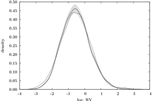
The descriptive statistics of the resulting realized volatility series are presented in Table 1. In summary, the empirical characteristics of the series are in line with the findings reported in the earlier literature on realized volatility. In particular, realized volatility is strongly skewed and fat-tailed, while its logarithmic version is much closer to Gaussianity. This is also confirmed by the kernel density estimate of logarithmic realized volatility, which is presented in Figure 1 along with the kernel density

esti-0.00 0.05 0.10 0.15 0.20 0.25 0.30 0.35 0.40 0.45 0.50 -4 -3 -2 -1 0 1 2 3 4 density log. RV

Figure 1: Kernel density estimate of logarithmic realized volatility of the S&P500 in-dex futures (solid line). The shaded area corresponds to the pointwise 95% confidence intervals and the dashed line represents the kernel density estimate of i.i.d. random variables simulated from the fitted normal distribution.

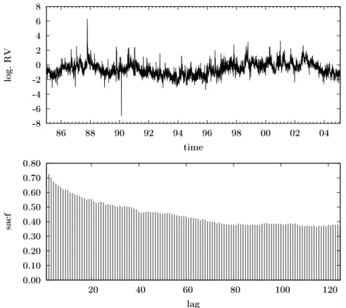
mate of i.i.d. random variables simulated from the fitted normal distribution (with a sample size corresponding to the empirical one). Moreover, the sample autocorrela-tion funcautocorrela-tion of (logarithmic) realized volatility (depicted in the lower panel of Figure

2) exhibits the aforementioned hyperbolic decay. We evaluate this long memory di-agnosis in more detail in the empirical application. In the following, however, we first introduce our localized approach to realized volatility modeling.

3

The localized realized volatility approach

An alternative view on the long memory phenomenon of volatility is given by a localization of the realized volatility dynamics. The idea of this localized approach for modeling realized volatility is as follows. It is assumed that at each point in

0.00 0.10 0.20 0.30 0.40 0.50 0.60 0.70 0.80 20 40 60 80 100 120 sacf lag -8 -6 -4 -2 0 2 4 6 8 86 88 90 92 94 96 98 00 02 04 log. RV time

Figure 2: Time evolvement and sample autocorrelation function (sacf) of logarithmic realized volatility of the S&P500 index futures.

time there exists a past time interval over which volatility can be approximated by a local autoregressive model of order one (LAR(1)) with constant parameters. In contrast to fitting a global volatility model, this implies that we obtain at each point in time a potentially new set of parameters, which is estimated based on the so–called interval of homogeneity. This technique, thus, also involves the determination of the length of this interval over which the parameters of the local model are assumed to be constant. Once the interval length and the parameters are determined for a particular time period, the corresponding local model may be used for volatility predictions. This section describes the adaptive estimation and the implementation of the localized approach in more detail. The performance is also tested in a set of simulation experiments.

3.1

Adaptive estimation method

The local (varying) autoregressive scheme of order 1 is defined through a time-varying parameter set θt= (θ1t, θ2t, θ3t)>:

logRVt =θ1t+θ2tlogRVt−1 +εt, εt ∼N(0, θ32t). (5)

Here the Gaussian distributed innovations εt have a mean of zero and variance θ32t.

time-varying parameters at any point in time t are of course too flexible to really

constitute a practical dynamic model. We therefore need to strike a balance between model flexibility and dimensionality. This is done by localizing a low dimensional time series dynamics in the high dimensional model (5).

The basic idea is to approximate (5) at a fixed time point τ by a parameter set θτ = (θ1τ, θ2τ, θ3τ)>, where θτ is constant over the interval Iτ = [τ −s, τ) with

0< s < τ. The intervalIτ defines a “locally homogeneous” span of data and is called

“interval of homogeneity”. The question is how to findIτ or the value ofs over which

the model parameters are estimated.

To this end, consider first the maximum likelihood (ML) estimator ˜θτ given an

homogeneous interval Iτ: ˜ θτ = argmaxθ∈ΘL(logRV;Iτ, θ) = argmax_θ∈Θ ( −s 2log 2π−slogθ3− 1 2θ2 3 τ−1 X t=τ−s (logRVt−θ1−θ2logRVt−1)2 )

where Θ denotes the parameter space and L(logRV;Iτ, θ) the local conditional

log-likelihood function. We, thus, refer to this estimator as the local ML estimator. For notational simplification, we also use the short notation L(Iτ, θ) for the local

Let the (logarithmic) realized volatility be exactly modelled by an AR(1) process with parameterθ∗_τ at time pointτ, i.eθ∗_τ is constant over the IntervalIτ. The accuracy

of estimation can then be measured by the log-likelihood ratio (LR):

LR(Iτ,θ˜τ, θτ∗) = L(Iτ,θ˜τ)−L(Iτ, θ∗τ). (6)

Polzehl and Spokoiny (2006) have proved that LR and its power transformation

|LR(Iτ,θ˜τ, θτ∗)|rwithr >0 are bounded for an i.i.d. sequence of Gaussian innovations

(in our case this refers to the innovations of the local AR(1) process):

Eθ∗ τ LR(Iτ, ˜ θτ, θ∗τ) r ≤ξr (7) with ξr = 2r R ξ≥0ξr

−1_e−ξ_{dξ = 2rΓ(r). This bound is non-asymptotic and allows to}

construct a confidence interval, which can be used to identify a homogeneous interval. The number of possible interval candidates is large, e.g. the first interval may include just a few past observations and the intervals considered thereafter may be increased by just one observation in each step up to including all past observations. As this is computationally intensive, especially for large data sets, we consider only a finite set of intervals Iτ ={Iτ1, . . . , IτK} with a reasonable value of K, as proposed in

Chen and Spokoiny (2009). The intervals are increasingly ordered according to their length, i.e. I1

τ ⊂ . . . ⊂ IτK. The first interval Iτ1 should be short enough such that

homogeneity can be assured. Note that to each interval there corresponds a local ML estimate, denoted by ˜θ_τk with k = 1, . . . , K. In statistical learning theory these are called weak learners. The risk bound (7) is calculated under the hypothetical constant θ_τ∗ parameter situation. By increasing the intervals in the nonparametric situation (5) we incur an increasing modeling bias. “Oracle” type of results as given in Belomestny and Spokoiny (2007) ensure that an optimal choice ˆIτ of an interval of

homogeneity (striking a balance between bias and variation) can be obtained via an adaptive procedure. Details of the “oracle” results can be found in the cited literature. The aim of this research is to put forward the mentioned dual view on the depen-dence structure of volatility. It is therefore appropriate here to concentrate on the construction details rather than on the theoretical technicalities. The main ingredient of the local model selection algorithm is based on a sequential testing procedure. The procedure starts from the shortest intervalI_τ1, where the homogeneity is assured and ˜

θ1

τ is automatically accepted as a homogeneous estimator: ˆθ1τ = ˜θτ1. Sequentially at

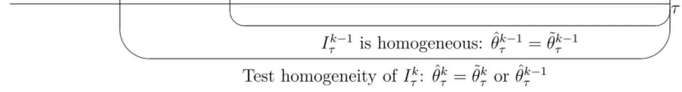
step k ≥ 2, we test the hypothesis of homogeneity of the successive interval Ik τ, see

Figure3. The test at step k is formulated as: LR(I k τ,θ˜ k τ,θˆ k−1 τ ) r ≤ ζk (8)

whereζkis the critical value (described in more detail below). The test is motivated by

the bound (7). The likelihood ratio measures the difference of a new ML estimate ˜θk τ

over a “possibly” homogeneous intervalI_τk and the previously accepted homogeneous estimate ˆθk_τ−1. If there is no significant difference between the two estimates, we accept the new one ˆθk

τ = ˜θτk. The reason is that, compared to the former accepted

estimate ˆθk−1

τ , the new estimate has a smaller variation as more observations are used

in the estimation. On the other hand, if the difference is significant, it indicates that a structural shift rather than homogeneity is detected and the sequential testing terminates. The significance at each step is measured by a critical value. Therefore, a set of critical values {ζk}Kk=1 is required in the sequential testing. In the next

section, we discuss the computation of the critical values and the choice of the involved parameters.

& %

τ

I_τk−1 is homogeneous: ˆθ_τk−1 = ˜θ_τk−1 Test homogeneity of I_τk: ˆθ_τk= ˜θ_τk or ˆθk_τ−1

Figure 3: Sequential test of homogeneity: the longer interval Ik

τ is tested after the

hypothesis of homogeneity over the shorter interval I_τk−1 has been accepted.

1. Initialization: ˆθ1_τ = ˜θ_τ1. 2. k= 1 while LR(Iτ, ˜ θk+1 τ ,θˆkτ) r ≤ζk+1 and k < K, k = k+ 1 ˆ θk_τ = θ˜k_τ 3. Final estimate: ˆθτ = ˆθτk

3.2

Choice of parameters and implementation details

To run the proposed adaptive procedure, we need to determine the input parameters, i.e. the set of intervals, the power parameter r in (8) and the critical values. In the following we present our choices and the computation of the critical values using Monte Carlo simulation.

Set of intervals

We consider a finite set withK = 13 intervals. This set is composed of the following

interval lengths:

wherew denotes a week (5 days),m refers to one month (21 days) andy to one year (252 days). In other words, I_τ1 = [τ−1w, τ), I_τ2 = [τ −1m, τ), . . ., I_τ13 = [τ −5y, τ). Note that the same setI ={Ik

τ}13k=1 is used for each time pointτ and for notational

convenience we therefore drop the subscript in the following. Our interval choice is motivated by practical reason that investors are often concerned about special investment horizons. Using also different sets of intervals, we find that the procedure is insensitive to the interval choice. Nevertheless, it is important to assure homogeneity over the shortest interval.

Critical values

In the testing procedure, the critical values measure the significance of the ML es-timate under the hypothesis of homogeneity. We here calculate the critical values under homogeneity, i.e. constant parameters in (5). In particular, we generate 100 000 AR(1) processes with θt = θ∗ = (θ1∗, θ∗2, θ3∗)> for all t: yt = θ1∗+θ2∗yt−1+εt,

εt ∼ N(0, θ∗32). The starting value was set to y0 = θ∗1/(1−θ ∗

2). The sample size of

each process is 1261 (corresponding to 5 years and 1 day) in accordance to the largest interval of I. Clearly the ML estimate of the largest interval (I13) is the choice, i.e. ˆ

θt = ˆθKt = ˜θtK. Remember that in the sequential testing the adaptive estimator at

step k depends on the critical values {ζ1, . . . , ζk} and we therefore use the notation

ˆ θk_t(ζ

1,...,ζk) to emphasize the effect of the critical values. The estimate ˆθ

K

t is required to

fulfill the following risk bound:

Eθ∗ LR IK,θ˜_tK,θˆ_tK_(ζ1,...,ζ K) r ≤ξr (9)

Moreover, it has been discussed in the non- and semiparametric literature that an increase in sample size implies an increase of bias due to the increase in degrees of freedom, see e.g. H¨ardle, M¨uller, Sperlich and Werwatz (2004). To take this into

account, we introduce a weighting scheme for k = 1, . . . , K into the risk bound, i.e.: Eθ∗ LR Ik,θ˜k_t,θˆ_tk_(ζ 1,...,ζk) r ≤ k−1 K−1ξr (10)

The weight (k−1)/(K −1) reflects the nature of the bias increase. It is also worth mentioning that the above expressions deviate from (7), i.e. the adaptive estimator replaces the parameter set θ∗. The bias due to this replacement is controlled for by

the critical values.

The sequential testing procedure is adopted to compute the critical values. At stepk = 1, we setζ1 =∞in agreement with the homogeneity of the shortest interval I1, which delivers the result ˆθ1_t = ˜θ1_t. In selection of ζ2, we set all the remaining ζk =∞ for k ≥3 to specify the contribution of ζ2. We choose the minimal value of ζ2 satisfying the following risk function:

Eθ∗ LR Ik,θ˜k_t,θˆk_t(ζ 1,ζ2) r ≤ 1 K−1ξr, k= 2, . . . , K.

Consequently with ζ1, ζ2, . . . , ζk−1 fixed, we select the minimal value of ζk for k =

3, . . . , K which fulfills: Eθ∗ LR Il,θ˜l_t,θˆ_tl_{(ζ1,ζ2,...,ζk)} r ≤ k−1 K−1ξr, l =k, . . . , K.

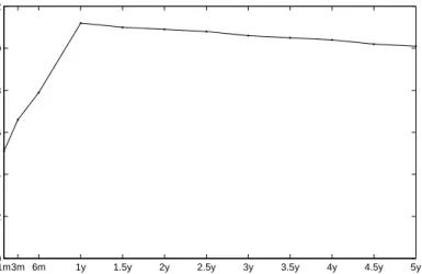
Figure4depicts the critical values calculated for the simulated AR(1) processes with θ∗ = (−0.1197,0.7754,0.5634)>. The parameters correspond to our real data set, i.e. they are estimates of an AR(1) model fitted to the logarithm of realized volatility of the S&P500 index data.

The choice of critical values depends on the parameterr. Belomestny and Spokoiny

simu-1m3m 6m 1y 1.5y 2y 2.5y 3y 3.5y 4y 4.5y 5y 0 2 4 6 8 10 12 Length of interval Critical values

Figure 4: The set of critical values. They are based on r = 1/2 and on θ∗ = (−0.1197,0.7754,0.5634)>, which are calculated for the log realized volatility of the S&P500 index futures under the hypothesis of constant parameters in (5). The set of interval lengths is given on the X-axis.

lation, we here follow their recommendation. Note that the critical values also rely on the parameter θ∗ in the simulation. In our study, we discuss two ways for

se-lecting θ∗: in the first θ∗ is estimated over the full sample period, whereas in the

secondθ∗ is estimated at each time point using a rolling window with a fixed length.

In general, a large rolling window size means that we put more attention to a time homogeneous situation. Such a choice leads to a rather conservative procedure with possibly low accuracy of estimation. On the contrary, a rolling window including fewer observations is more sensitive to structural shifts. The size of rolling window can be selected in a data driven way by minimizing some objective function, e.g., by minimizing the forecasting error. In Section 5 we report the prediction performance using both a constant set of critical values over all the observations and the time dependent sets with rolling windows including 1-month, 6-month, 1-year and 2.5-year observations. As expected, using the time dependent critical values increases the accuracy of prediction.

3.3

Simulation experiments

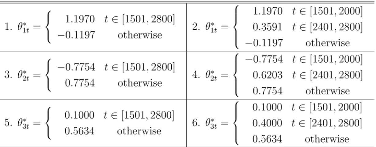
This section reports the performance of the adaptive estimation in a number of sim-ulation experiments. The focus is the reaction of the new technique to a shift of parameters. The parameters estimated for the full S&P 500 realized volatility data serves again as a guidance. Several scenarios are studied here (see Table2), by which one parameter varies over some time periods while the other two remain constant. Different size of shifts (big or small) followed by homogeneous intervals with different lengths (long and short) are examined. For example, case 1 involves a big shift inθ1t,

the intercept of the LAR(1) process, over a long homogeneous time span [1501,2800].

For each case, we generated 500 LAR(1) processes with 3260 observations. The first 1260 observations, corresponding to I13 = 5 years, are used as training set. The

Table 2: Scenarios of the simulation study

1. θ∗_1t=    1.1970 t∈[1501,2800] −0.1197 otherwise 2. θ ∗ 1t=        1.1970 t ∈[1501,2000] 0.3591 t ∈[2401,2800] −0.1197 otherwise 3. θ∗_2t=    −0.7754 t∈[1501,2800] 0.7754 otherwise 4. θ ∗ 2t=        −0.7754 t ∈[1501,2000] 0.6203 t ∈[2401,2800] 0.7754 otherwise 5. θ∗_3t=    0.1000 t ∈[1501,2800] 0.5634 otherwise 6. θ ∗ 3t=        0.1000 t∈[1501,2000] 0.4000 t∈[2401,2800] 0.5634 otherwise

Note: in each of the 6 scenarios only one parameter is changed either once or twice. The remaining ones are fixed to the values estimated from the full S&P500 realized volatility data, i.e. (−0.1197,0.7754,0.5634)>.

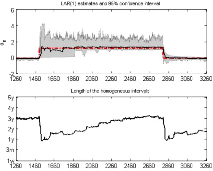
average value of the estimated parameters (solid line) and the pointwise 95% confi-dence intervals (shaded areas) are displayed in Figures 5 to7. The true values of θ∗ (dashed line) are depicted for judgement. It shows that in many cases the method reacts quickly to a big shift but slowly to a small shift. For example as the intercept

Figure 5: Simulation results forθ1t: The red dashed line represents the process of the

true time-varying parameter and the bold solid line is the average values of the esti-mated parameter over 500 simulations. The shaded area corresponds to the pointwise 95% confidence intervals. The average values of the selected homogeneous intervals for each time point are presented below each case of simulations.

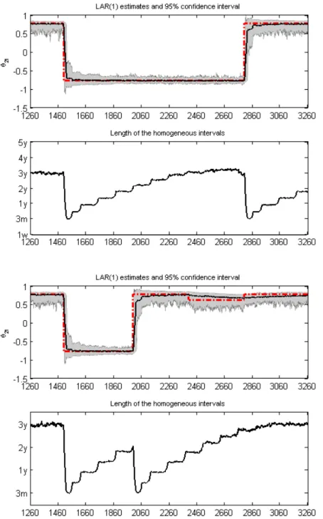
Figure 6: Simulation results forθ2t: The red dashed line represents the process of the

true time-varying parameter and the bold solid line is the average values of the esti-mated parameter over 500 simulations. The shaded area corresponds to the pointwise 95% confidence intervals. The average values of the selected homogeneous intervals for each time point are presented below each case of simulations.

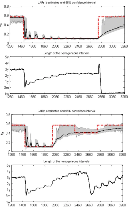
Figure 7: Simulation results forθ3t: The red dashed line represents the process of the

true time-varying parameter and the bold solid line is the average values of the esti-mated parameter over 500 simulations. The shaded area corresponds to the pointwise 95% confidence intervals. The average values of the selected homogeneous intervals for each time point are presented below each case of simulations.

θ1t jumps at t = 1500, it needs 20 steps to catch up 70% of the big shift. For the

small shift at t= 2400, the procedure needs roughly 254 steps, see Figure 5. Similar results are obtained for the shifts inθ2t. However, positive shifts inθ3t, corresponding

to an increase in the signal-to-noise ratio, are only slowly detected, see Figure7. The average values of the selected homogeneous intervals over the simulations for each time point are presented below each case, see Figures5to Figure7. As expected, the homogeneous intervals are long when the parameters remain constant and become short sharply after a shift. It is also observed that the length of homogenous intervals seems to have no considerable influence on the adaptive estimation.

4

Long memory models

As we aim at a comparison to the long memory view of volatility, we briefly review here the most popular realized volatility models emanating from this view.

In contrast to the fractionally integrated GARCH models, in which volatility is a function of the daily squared return innovations that exhibits a hyperbolically de-caying autocorrelation, the realized volatility literature applies fractionally integrated processes directly to the (more precise) realized volatility measure. Andersen et al. (2003), for example advocated the use of an ARFIMA(p, q) for modeling (logarithmic)

realized volatility. The ARFIMA(p, q) model is given by

φ(L)(1−L)d(logRVt−µ) =ψ(L)ut, (11)

with φ(L) = 1−φ1L−. . .−φpLp,ψ(L) = 1 +ψ1L+. . .+ψqLq, L denoting the lag

operator, and d∈(0,0.5) is the fractional difference parameter. Given the empirical distributional properties of logarithmic realized volatility, ut is usually assumed to

be a Gaussian white noise process, which facilitates the exact maximum-likelihood estimation of the model.

The HAR model aims at reproducing the observed volatility phenomenon. How-ever, in contrast to the ARFIMA model, the HAR model is formally not a long memory model. Instead, the correlation structure is approximated by the sum of a few multi-period volatility components. The use of such components is motivated by the existence of heterogenous agents having different investment horizons (see Corsi, 2008; M¨uller, Dacorogna, Dav, Olsen, Pictet and von Weizs¨acker, 1997). In particular, the HAR model put forward by Corsi (2008) builds on a daily, weekly and monthly component, which are defined by:

RVt+1−k:t = 1 k k X j=1 RVt−j. (12)

with k = 1,5,21, respectively. The HAR model is then given by

logRVt = α0+αdlogRVt−1+αwlogRVt−5:t−1+αmlogRVt−21:t−1+ut(13)

with ut typically being also Gaussian white noise. Maximum-likelihood estimation

is straightforward. Interestingly, the HAR and ARFIMA models have been found to obtain a similar forecasting performance with both models outperforming the tra-ditional volatility models based on daily returns (for the latter see e.g. Andersen, Bollerslev and Diebold, 2007; Koopman, Jungbacker and Hol, 2005).

5

Empirical analysis

We now turn to the empirical investigation of the dual views on the dynamics of volatility. We focus our analysis on realized volatility of the S&P500 index futures

from January 2, 1985 to February 4, 2005 (see Section 2). Like in the simulation exercise we use the first 5 years of our sample as a training set. For the local autore-gressive procedure this means that January 2, 1990 is the first time point for which we estimate the LAR(1) model and that we allow the longest interval of homogene-ity (K = 13) to be 5 years with the remaining set of subintervals given as in the

simulation part, i.e. 1 week (k = 1), 1 month (k = 2), . . ., 4.5 years (k = 12).

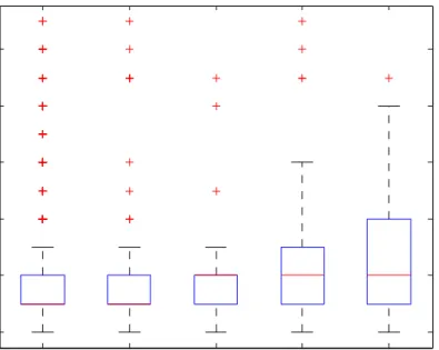
We estimate the LAR(1) model based on different sets of critical values. In partic-ular, we first consider critical values obtained from a Monte Carlo simulation based on the parameter values of an AR(1) model being estimated over the full sample period. We refer to this as the global LAR(1) model. The other sets of critical values are obtained adaptively using a 1 month, 6 months, 1 year and 2.5 years sample period. Figure 8 shows the distribution of the lengths of the selected homogenous intervals over the evaluation period (January 2, 1990 to February 4, 2005) based on the global and the adaptive critical values, respectively. Obviously, the global LAR(1) model ex-hibits a slightly higher variation in the length of the selected intervals. Nevertheless, the average interval length is for nearly all LAR(1) models about 6 months, which indicates only a weak sensitivity of the interval selection procedure to the sample size used in the computation of the critical values. Interestingly, with the exception of the adaptive 1 month and 6 months LAR(1) models for which the median interval length is at k = 3, we find that the median is k = 4, which corresponds to 6 months

of homogeneity.

We investigate the dual views by comparing the forecasting performance of the localized realized volatility procedure to ARFIMA and HAR models. To this end, we recursively compute one-step-ahead (logarithmic) realized volatility forecasts from all three model types over the evaluation period. We compute the ARFIMA and HAR forecasts based on a rolling window scheme, i.e. each forecast is based on an estimation

1m 6m 1y 2.5y global 1m 6m 1.5y 2.5y 3.5y 4.5y

Length of selected homogeneous interval

Rolling window used to adapt critical values

Figure 8: Boxplot of the homogenous intervals selected by the LAR(1) procedure with 1 month, 6 months, 1 year, 2.5 years adaptive critical values and the global LAR(1) procedure.

of the model over a constant number of observations. As it is sometimes argued, that both long memory and structural breaks are driving volatility, we attempt to account for this possibility by considering also smaller window sizes. Overall, we use 11 rolling window sizes ranging from 3 months to 5 years, which is broadly consistent with our choice of subintervals in the LAR(1) procedure. We additionally consider forecasts from constant AR(1) models based on the same rolling windows, as this allows for a direct evaluation of the relevance of the localization in our LAR(1) procedure. Recall, that the individual forecasts from the LAR(1) model are based on varying estimation periods, i.e. on the lengths of the homogenous time intervals that are selected at the forecast origins.

Table 3shows the root mean square forecast errors (RMSFE) and the mean abso-lute forecast error (MAE) of the various models. Note, that the ARFIMA forecasts

Table 3: Forecast evaluation criteria

Sample period RMSFE MAE

LAR(1) LAR(1)

local adaptive 1m 0.4858 - - 0.3667 -

-local adaptive 6m 0.4811 - - 0.3654 -

-local adaptive 1y 0.4876 - - 0.3704 -

-local adaptive 2.5y 0.4916 - - 0.3748 -

-local global 0.5014 - - 0.3824 -

-AR(1) ARFIMA HAR AR(1) ARFIMA HAR

3m 0.5149 0.5328 0.5381 0.3900 0.3978 0.4025 6m 0.5288 0.5225 0.5240 0.3987 0.3902 0.3862 1y 0.5398 0.5178 0.5185 0.4057 0.3860 0.3857 1.5y 0.5462 0.5143 0.5172 0.4103 0.3836 0.3843 2y 0.5509 0.5133 0.5158 0.4136 0.3826 0.3836 2.5y 0.5555 0.5132 0.5153 0.4157 0.3816 0.3839 3y 0.5574 0.5123 0.5155 0.4177 0.3814 0.3843 3.5y 0.5607 0.5132 0.5164 0.4202 0.3820 0.3859 4y 0.5649 0.5129 0.5171 0.4238 0.3817 0.3851 4.5y 0.5686 0.5130 0.5173 0.4273 0.3821 0.3854 5y 0.5712 0.5129 0.5176 0.4300 0.3819 0.3858

The table reports the forecast evaluation criteria for 1-day-ahead forecast of the logarithmic realized variance of the S&P500 index futures based on the LAR(1), the constant AR(1), the ARFIMA and the HAR models. The first column refers either to the sample period used in the computation of the critical values in the LAR(1) procedure or to the rolling window sizes. Bold numbers indicate the minimum of the forecast evaluation criteria within each model class.

are based on an ARFIMA(2,d,0) specification, which was selected according to the

Akaike as well as the Bayesian information criteria using the full sample period. Estimation and forecasting is carried out using the Ox ARFIMA 1.04 package, see Doornik and Ooms (2004), Doornik and Ooms (2006). Interestingly, our LAR(1) procedure provides the most accurate forecasts. This holds already for the forecasts based on the LAR(1) model with globally computed critical values. The performance can be further improved using adaptive critical values. More precisely, a reduction of

the sample period underlying the computation of the critical values introduces more flexibility into the procedure, which seems to result in an (albeit somewhat small) increase in forecast accuracy.

The direct comparison of the LAR(1) forecasts with those based on the constant AR(1) models also reveals, that the adaptive local selection of the homogenous in-tervals is indeed important. Obviously, the adaptive procedure, which determines at each time point the adequate length of the time interval over which the AR(1) model is appropriate, is superior. Noteworthy, for increasing window sizes the predictability of the constant AR(1) model worsens. This might be expected as for larger sam-ple sizes, e.g. more than 2 years, the autocorrelation function of realized volatility exhibits more persistence and, thus, an AR(1) model tends to be misspecified.

For the same reason it is not surprising that the predictive performance of the long memory models increases when we consider larger rolling windows. Note also, that in accordance to the empirical results reported in the realized volatility litera-ture so far, the HAR and ARFIMA models exhibit similar forecast accuracy with a slight tendency of the ARFIMA model to outperform the HAR model. Both models, however, are outperformed by the localized realized volatility method.

We further evaluate the predictive performance of the different realized volatility models on the grounds of the so–called Mincer–Zarnowitz regressions, i.e. by re-gressing the observed logarithmic realized volatility on the corresponding forecasts of model i:

logRVt=α+βlogdRV_t,i+ν_t. (14)

This allows us to test for the unbiasedness of the different forecasts. Table 4 reports the regression results along with the p-value of the F-test on unbiased forecasts, i.e.

Table 4: Mincer-Zarnowitz regression results for log. realized volatility Model α β p-value R2 global LAR −0.0130 (0.0125) 1.0128 (0.0142) 0.1007 0.6959 adaptive LAR, 1y 0.0025 (0.0123) 1.001 (0.0127) 0.9780 0.7117 1y AR(1) −0.0010 (0.0144) 1.0117 (0.0158) 0.6002 0.4669 5y AR(1) 0.0221 (0.0162) 1.0367 (0.0213) 0.2216 0.6052 1y ARFIMA 0.0008 (0.0119) 1.001 (0.0132) 0.9962 0.6747 5y ARFIMA 0.0009 (0.0115) 1.0154 (0.0129) 0.4907 0.6811 1y HAR −0.0076 (0.0128) 0.9907 (0.0128) 0.7509 0.6742 5y HAR 0.0145 (0.0119) 1.0237 (0.0133) 0.2036 0.6756

Reported are the estimation results of the Mincer-Zarnowitz regres-sions with heteroscedasticity and autocorrelation robust Newey-West standard errors given in parentheses. The third column reports the

p-value of an F-test forH0: α= 0 andβ= 1.

forecasts based on a moderately small sample (1 year) and a large sample (5 years). Correspondingly, we only consider the LAR(1) models based on the 1 year adaptively and on the globally computed critical values.

The results indicate that none of the forecasts is significantly biased at the 5% sig-nificance level. Noteworthy, the adaptive computation of the critical values seems to result in less systematic forecast errors. Similarly, the long memory and the constant AR(1) models exhibit smallerp-values for larger window sizes. The regression

coeffi-cients reported in Table4indicate a superior forecasting performance of the adaptive LAR(1) models. We investigate this result further and test for the significance of the observed differences in the forecast accuracies. In particular, we conduct a pairwise

test on the equality of the mean square forecast errors (MSFE) of the LAR(1) proce-dure and the other models (see Diebold and Mariano, 1995). To this end, we regress the difference between the squared forecast errors of the LAR(1) model and those of the competing model i, i.e. e2

t,LAR −e2t,i, on a constant µ. The null hypothesis of

equal MSFEs is equivalent to H0 : µ = 0. Table 5 presents the test results.

Obvi-ously, the null hypothesis is always rejected in favor of a significant better forecasting performance of the adaptive LAR(1) model, as indicated by the significant negative estimate of µ. For the global LAR(1) model, however, we fail to reject the null.

6

Conclusion

This paper investigates a dual view on the long range dependence of realized volatility. While the current literature primarily advocates the use of long memory models to explain this phenomenon, we argue that volatility can alternatively be described by short memory models with structural breaks. To this end we propose the localized approach to realized volatility modeling where we consider the case of a dynamic short memory model. In particular, at each point in time we determine an interval of homogeneity over which the volatility is approximated by an AR(1) process. Our approach is based on local adaptive techniques developed in Belomestny and Spokoiny (2007), which make it flexible and allows for arbitrarily time-varying coefficients. This contrasts to smooth transition or regime switching models. Our procedure relies on parameters, that have to be predetermined but allow more flexibility. In particular, we show, that an adaptive view on intervals of homogeneity (and a decrease in the respective underlying sample size) is increasing the procedure’s flexibility, yielding higher accuracy in estimation and a better forecasting performance. Furthermore, the choice of the underlying parameters can also be based upon criteria reflecting the

Table 5: Diebold Mariano test results

compared models µ

(global LAR)-(1y AR(1)) −0.0400

(0.0096)

(global LAR)-(5y AR(1)) −0.0141

(0.0109)

(global LAR)-(1y ARFIMA) −0.0168

(0.0109)

(global LAR)-(5y ARFIMA) −0.0118

(0.0109)

(global LAR)-(1y HAR) −0.0175

(0.0104)

(global LAR)-(5y HAR) −0.0165

(0.0104)

(adaptive LAR, 1y)-(1y AR(1)) −0.0535

(0.0097)

(adaptive LAR, 1y)-(5y AR(1)) −0.0546

(0.0111)

(adaptive LAR, 1y)-(1y ARFIMA) −0.0304

(0.0108)

(adaptive LAR, 1y)-(5y ARFIMA) −0.0253

(0.0109)

(adaptive LAR, 1y)-(1y HAR) −0.0310

(0.0103)

(adaptive LAR, 1y)-(5y HAR) −0.0258

(0.0103)

Reported are test results for the Diebold Mariano test on equal fore-cast performance, i.e. H0 : µ= 0 in the regression e2t,LAR−e2t,i =

µ+vtwithet,idenoting the forecast error of modeli.

Heteroscedastic-ity and autocorrelation robust Newey-West standard errors are given in parentheses.

user’s objective, such as in sample fit or forecasting criteria. Although we have re-frained from doing so in our empirical application, we find that our adaptive localized realized volatility procedure provides accurate volatility forecasts and significantly outperforms the standard long memory realized volatility models. It seems that our alternative view on volatility is practical and realistic. Our forecast evaluation further suggests, that the adaptive localization is an important feature of our procedure, i.e. the locally adaptive selection of the homogenous intervals is superior to the specifi-cation of a short memory model that is assumed to be constant over a globally fixed period, such as e.g. an AR(1) model based on fixed rolling window sizes.

References

Andersen, T., Bollerslev, T., Diebold, F. and Ebens, H. (2001a). The distribution of realized stock return volatility, Journal of Financial Economics61: 43–76. Andersen, T. G. and Bollerslev, T. (1998). Answering the skeptics: Yes, standard

volatility models do provide accurate forecasts, International Economic Review

39: 885–905.

Andersen, T. G., Bollerslev, T. and Diebold, F. X. (2007). Roughing it up: Includ-ing jump components in the measurement, modelInclud-ing and forecastInclud-ing of return volatility,Review of Economics and Statistics 89: 701–720.

Andersen, T. G., Bollerslev, T., Diebold, F. X. and Labys, P. (2001b). The distri-bution of realized exchange rate volatility, Journal of the American Statistical

Association 96: 42–55.

Andersen, T. G., Bollerslev, T., Diebold, F. X. and Labys, P. (2003). Modeling and forecasting realized volatility, Econometrica 71: 579–625.

Baillie, R. T., Bollerslev, T. and Mikkelsen, H. O. (1996). Fractionally integrated gen-eralized autoregressive conditional heteroskedasticity, Journal of Econometrics

74: 3–30.

Bandi, F. M. and Russell, J. R. (2005). Microstructure noise, realized volatility, and optimal sampling,Review of Economic Studies 75: 339–369.

Barndorff-Nielsen, O. E. and Shephard, N. (2002a). Econometric analysis of realized volatility and its use in estimating stochastic volatility models, Journal of the

Royal Statistical Society B64: 253–280.

Barndorff-Nielsen, O. E. and Shephard, N. (2002b). Estimating quadratic variation using realized variance, Journal of Applied Econometrics17: 457–477.

Barndorff-Nielsen, O. E., Hansen, P. R., Lunde, A. and Shephard, N. (2008). De-signing realised kernels to measure the ex-post variation of equity prices in the presence of noise, Econometrica 76: 1481–1536.

Belomestny, D. and Spokoiny, V. (2007). Spatial aggregation of local likelihood esti-mates with applications to classification,The Annals of Statistics35: 2287–2311. Chen, Y. and Spokoiny, V. (2009). Modeling and estimation for nonstationary time

series with applications to robust risk management,submitted. ˇ

C´ıˇzek, P., H¨ardle, W. and Spokoiny, V. (2009). Statistical inference for time-inhomogeneous volatility models, submitted.

Corsi, F. (2008). A simple long memory model of realized volatility, Journal of

Financial Econometrics. forthcoming.

Diebold, F. and Mariano, R. (1995). Comparing predictive accuracy, Journal of

Diebold, F. X. and Inoue, A. (2001). Long memory and regime switching,Journal of

Econometrics 105: 131–159.

Doornik, J. A. and Ooms, M. (2004). Inference and forecasting for arfima models, with an application to us and uk inflation, Studies in Nonlinear Dynamics and

Econometrics 8: Article 14.

Doornik, J. A. and Ooms, M. (2006). A package for estimating, fore-casting and simulating arfima models: Arfima package 1.04 for ox,

http://www.doornik.com/download.html.

Granger, C. W. and Joyeux, R. (1980). An introduction to long memory time series models and fractional differencing, Journal of Time Series Analysis 1: 5–39. Granger, C. W. J. (1980). Long memory relationships and the aggregation of dynamic

models, Journal of Econometrics 14: 227–238.

Granger, C. W. J. and Hyung, N. (2004). Occasional structural breaks and long memory with an application to the s&p 500 absolute stock returns, Journal of

Empirical Finance 11: 399–421.

Hansen, P. R. and Lunde, A. (2006). Realized variance and market microstructure noise, Journal of Business and Economic Statistics24: 127–161.

H¨ardle, W., M¨uller, M., Sperlich, S. and Werwatz, A. (2004). Nonparametric and

Semiparametric Models, Springer Verlag.

Hosking, J. R. M. (1981). Fractional differencing, Biometrika 68: 165–176.

Koopman, S. J., Jungbacker, B. and Hol, E. (2005). Forecasting daily variability of the S&P 100 stock index using historical, realised and implied volatility mea-surements,Journal of Empirical Finance 12: 445–475.

Mikosch, T. and St˘aric˘a, C. (2004a). Changes of structure in financial time series and the GARCH model,REVSTAT Statistical Journal 2: 41–73.

Mikosch, T. and St˘aric˘a, C. (2004b). Non-stationarities in financial time series, the long range dependence and the IGARCH effects, Review of Economics and

Statistics 86: 378–390.

M¨uller, U. A., Dacorogna, M. M., Dav, R. D., Olsen, R. B., Pictet, O. V. and von Weizs¨acker, J. E. (1997). Volatilities of different time resolutions - analyzing the dynamics of market components, Journal of Empirical Finance 4: 213–239. Polzehl, J. and Spokoiny, V. (2006). Propagation-separation approach for local

like-lihood estimation,Probability Theory and Related Fields 135: 335–362.

Pong, S., Shackleton, M. B., Taylor, S. J. and Xu, X. (2004). Forecasting currency volatility: A comparison of implied volatilities and AR(FI)MA models, Journal

of Banking & Finance 28: 2541–2563.

Zhang, L., Mykland, P. A. and A¨ıt-Sahalia, Y. (2005). A tale of two time scales: Determining integrated volatility with noisy high-frequency data, Journal of the

American Statistical Association 100: 1394–1411.

Zhou, B. (1996). High-frequency data and volatility in foreign-exchange rates,Journal

SFB 649 Discussion Paper Series 2009

For a complete list of Discussion Papers published by the SFB 649, please visit http://sfb649.wiwi.hu-berlin.de.

001 "Implied Market Price of Weather Risk" by Wolfgang Härdle and Brenda López Cabrera, January 2009.

002 "On the Systemic Nature of Weather Risk" by Guenther Filler, Martin Odening, Ostap Okhrin and Wei Xu, January 2009.

003 "Localized Realized Volatility Modelling" by Ying Chen, Wolfgang Karl Härdle and Uta Pigorsch, January 2009.

SFB 649, Spandauer Straße 1, D-10178 Berlin http://sfb649.wiwi.hu-berlin.de