NONPARAMETRIC PRICING KERNEL MODELS
by Linman Sun
A dissertation submitted to the faculty of the University of North Carolina at Charlotte
in partial fulfillment of the requirements for the degree of Doctor of Philosophy in
Applied Mathematics Charlotte 2011 Approved by: Dr. Zongwu Cai Dr. Weihua Zhou Dr. Jiancheng Jiang Dr. Lisa S.Walker
c °2011 Linman Sun
iii ABSTRACT
Linman Sun. Nonparametric Pricing Kernel Models. (Under the direction of DR. ZONGWU CAI)
The capital asset pricing model (CAPM) and the arbitrage asset pricing theory (APT) have been the cornerstone in theoretical and empirical finance for the recent few decades. The classical CAPM usually assumes a simple and stable linear relationship between an asset’s systematic risk and its expected return. However, this simple relationship assumption has been challenged and rejected by several recent studies based on empirical evidences of time variation in betas and expected returns.
It is well documented that large pricing errors could be due to the linear ap-proach used in a nonlinear model and treating a non-linear relationship as a linear could lead to serious prediction problems in estimation. To overcome these problems, in the first part of this dissertation I would like to investigate a general nonpara-metric asset pricing model to avoid functional form misspecification of betas, risk premia, and the stochastic discount factor by considering estimating unknown func-tional involved in the nonparametric pricing kernel. To estimate the nonparametric functionals, I propose a new nonparametric estimation procedure, termed as non-parametric generalized estimation equations (NPGEE), which combines the local linear fitting and the generalized estimation equations. I establish the asymptotic properties of the resulting estimator. Also, as a rule of thumb, I propose a data-driven method to select the bandwidth and provide a consistent estimate of the asymptotic variance.
The nonparametric method may provide a useful insight for further parametric fitting, while parametric models for time-varying betas can be most efficient if the underlying betas are specified. However, a misspecification may cause serious bias
and model constraints may distort the betas in local area. Hence, to test whether the pricing kernel model has some specific parametric form becomes essentially impor-tant. In the second part of this dissertation, I propose a consistent nonparametric testing procedure to test whether the model is correctly specified and I establish the asymptotic properties of the test statistic using a U-statistic technique.
Finite sample results are investigated using Monte Carlo simulation studies in order to show the usefulness of the estimation method and the test statistics. The empirical applications using CRSP monthly returns are also implemented to illustrate our proposed models and methods.
v ACKNOWLEDGEMENTS
First of all, I would like to express my deep appreciation to my advisor Dr. Zongwu Cai. His excellent guidance, caring and patience played an important role throughout my Ph.D. study. Besides providing me with an effective guidance on my research, his enthusiasm to work also inspired me to push myself for better. This dissertation would not be possible without his guidance and encouragement.
Appreciation also extends to Dr. Jiancheng Jiang, Dr. Weihua Zhou, and Dr. Lisa S. Walker for serving as very valuable members in my advisory committee.
Finally, my special gratitude goes to my p parents Zhenying Sun and Kunyu Yang for their endless love, encouragement, and support throughout my life. To them I dedicate this dissertation.
TABLE OF CONTENTS
LIST OF FIGURES viii
LIST OF TABLES ix
CHAPTER 1: INTRODUCTION 1
1.1 Background and Motivation 1
1.2 Asset Pricing Models 3
1.2.1 CAP Model 4
1.2.2 Valuation Theory 6
1.2.3 Stochastic Discount Factor 7
1.2.4 Conditional Asset Pricing Models 9
1.2.5 Flexible SDF Models 14
1.3 Overview 16
CHAPTER 2: NONPARAMETRIC ASSET PRICING MODELS 18
2.1 The Model 18
2.2 Nonparametric Estimation Procedure 20
2.3 Distribution Theory 23
2.3.1 Assumption 23
2.3.2 Large Sample Theory 24
2.4 Model Extension 27 2.4.1 Distribution Theorem 29 2.5 Empirical Examples 32 2.5.1 Simulated Examples 32 2.5.2 A Real Example 37 2.6 Proof of Theorems 41
vii CHAPTER 3: TEST OF MISSPECIFICATION OF PRICING KERNEL 59
3.1 Parametric Models 60
3.2 Estimation and Statistical Inference 62
3.3 Distribution Theory 66
3.3.1 Assumptions 66
3.3.2 Large Sample Theory 67
3.3.3 Comparing Nonparametric with Parametric Pricing Kernel 70
3.4 Empirical Examples 71 3.4.1 Simulated Examples 71 3.4.2 A Real Example 75 3.5 Proof of Theorems 78 CHAPTER 4: CONCLUSION 97 REFERENCES 98
LIST OF FIGURES
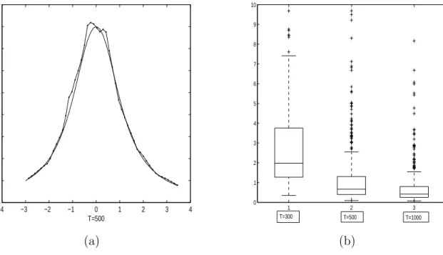
FIGURE 2.1 (a) The true curve of m(z) and its nonparametric estimate for sample size T = 500. (b) The boxplots of MADE500 for three sample sizes.
34
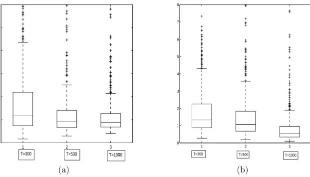
FIGURE 2.2 (a) The true curve of m(z) and its nonparametric estimate for sample size T = 500. (b) The boxplots of MADE500 for three sample sizes.
34
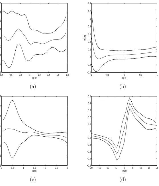
FIGURE 2.3 The boxplots of MADE500 for three sample sizes T = 300,
T = 500, T = 1000. (a) under mean-covariance efficiency; (b) without mean-covariance efficiency.
36
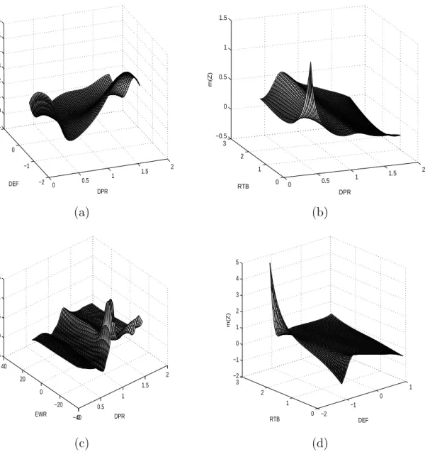
FIGURE 2.4 The one dimensional nonparametric estimate of m(·). (a) Zt is DPR; (b) Zt is DEF; (c)Zt is RTB; (d) Zt is EWR.
39
FIGURE 2.5 The two dimensional nonparametric estimate of m(·). (a) Zt =(DPR, DEF); (b)Zt=(DPR, RTB); (c)Zt =(DPR, EWR);
(d) Zt=(DEF, RTB).
40
ix LIST OF TABLES
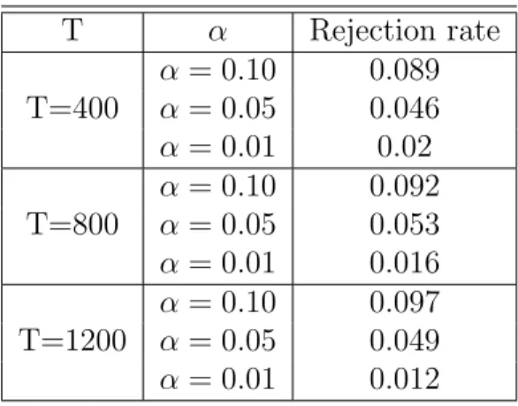
TABLE 3.1 Simulation results with three sample sizes T = 400, 800, 1200 for three significance levels α= 0.10, 0.05, and 0.01.
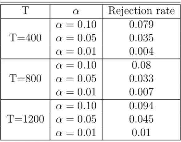
72 TABLE 3.2 Simulation results with three sample sizes T = 400, 800,
1200 for three significance levels α= 0.10, 0.05, and 0.01.
76
TABLE 3.3 Testing of the linearity 76
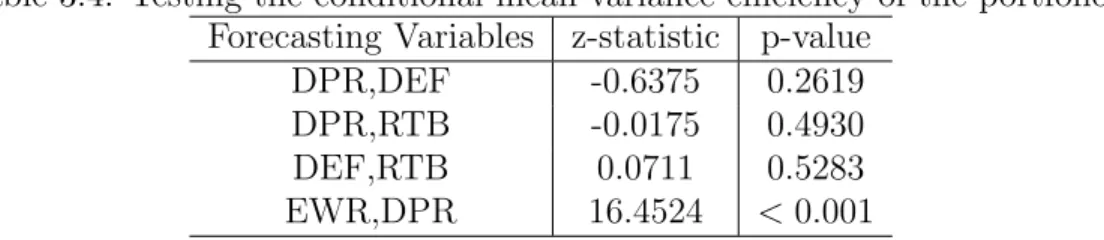
TABLE 3.4 Testing the conditional mean-variance efficiency of the port-folio.
1.1 Background and Motivation
The capital asset pricing (CAP) model and the arbitrage asset pricing theory (APT) have been the cornerstone in theoretical and empirical finance for the recent few decades. The classical CAPM usually assumes a simple and stable linear rela-tionship between an asset’s systematic risk and its expected return; see the books by Campbell, Lo and MacKinlay (1997) and Cochrane (2001) for details. However, this simple relationship assumption has been challenged and rejected by several recent studies based on empirical evidences of time variation in betas and expected returns (as well as return volatilities). As with other models, one considers the conditional CAP or nonlinear APT models with time-varying betas to characterize the time variation in betas and risk premia.
The recent work, to name just a few, includes Bansal, Hsieh and Viswanathan (1993), Bansal and Viswanathan (1993), Cochrane (1996), Jaganathan and Wang (1996, 2002), Reyes (1999), Ferson and Harvey (1991, 1993, 1998, 1999), Cho and Engle (2000), Wang (2002, 2003), Akdeniz, Altay-Salih and Caner (2003), Ang and Liu (2004), Fraser, Hamelink, Hoesli and MacGregor (2004), and the references therein. In particular, Fama and French (1992, 1993, 1995) used some instrumen-tal (fundameninstrumen-tal) variables like book-to-market equity ratio and market equity, as proxies for some unidentified risk factors to explain the time variation in returns, whereas Ferson (1989), Harvey (1989), Ferson and Harvey (1991, 1993, 1998, 1999), Ferson and Korajczyk (1995), and Jaganathan and Wang (1996) concluded that beta and market risk premium vary over time. Therefore, a static CAPM should
2 incorporate time variation in beta in the model.
Although there is a vast amount of empirical evidences on time variation in betas and risk premia, there is no theoretical guidance on how betas and risk premia vary with time or variables that represent conditioning information.
Many recent studies focus on modelling the variation in betas using continuous approximation and under the theoretical framework of the conditional CAPM; see, for example, Cochrane (1996), Jaganathan and Wang (1996, 2002), Wang (2002, 2003) and Ang and Liu (2004) and the references therein. Recently, Ghysels (1998) discussed the problem in detail and stressed the impact of misspecification of beta risk dynamics on inference and estimation. Also, he argued that betas change through time very slowly and linear factor models like the conditional CAPM may have a tendency to overstate the time variation. Furthermore, he showed that among several well-known time-varying beta models, a serious misspecification produces time variation in beta that is highly volatile and leads to large pricing errors. Finally, he concluded that it is better to use a static CAPM in pricing when one does not have a proper model to capture time variation in betas correctly.
It is well documented that large pricing errors may be due to the linear approach used in a nonlinear model and treating a nonlinear relationship as a linear can lead to serious prediction problems in estimation.
To overcome these problems, some nonlinear models have been considered in the recent literature. For example, Bansal, Hsieh and Viswanathan (1993) and Bansal and Viswanathan (1993) were the first to advocate the idea of a flexible stochastic discount factor (SDF) model in empirical asset pricing and they focused on nonlinear arbitrage pricing theory models by assuming that the SDF is a nonlinear function of a few of state variables. Also, Akdeniz, Altay-Salih and Caner (2003) tested for the existence of significant evidence of nonlinearity in the time series relationship of industry returns with market returns using the heteroskedasticity
consistent Lagrange multiplier test of Hansen (1996) under the framework of the threshold model and they found that there exists statistically significant nonlinearity in this relationship with respect to real interest rates. Furthermore, under the mean-covariance efficiency framework, Wang (2002, 2003) explored a nonparametric form of the SDF model and conducted a simple test based on the nonparametric pricing errors.
Gourieroux and Monfort (2007) considered a class of nonlinear parametric and semiparametric SDF models for derivative pricing by assuming that the stochastic discount factors are exponential-affine functions of underlying state variable. In particular, they discussed the conditionally Gaussian framework and introduced semiparametric pricing methods for models with path dependent drift and volatility. A nonparametric modeling is appealing in these situations. One of the advan-tages for nonparametric modeling is that no or little restrictive prior information on betas and pricing kernel is needed. Moreover, it may provide useful insight for further parametric fitting. Parametric models for time-varying betas and nonlinear pricing kernel can be most efficient if the underlying models are correctly speci-fied. However, a misspecification may cause serious bias and model constraints may distort the betas in local area.
In the following section, I give a brief introduction for famous asset pricing models.
1.2 Asset Pricing Models
Over the past decades, many studies have been conducted to examine the perfor-mance of SDF approach for econometric evaluation of asset-pricing models and CAP models in expected returns. As Jagannathan and Wang (2002) demonstrated, a clas-sical beta method or CAPM can be expressed as a SDF form. Also, as Cochrane (2001) pointed out, a SDF method is sufficiently general that it can be used for
4 analysis of linear as well as nonlinear asset-pricing models, including pricing models for derivative securities. Now I give a brief review about the CAP model and SDF form.
1.2.1 CAP Model
The basic theorem of capital asset pricing model (CAPM) and portfolio selection problem were proposed by Markovitz (1959). Investors would optimally hold a mean-variance efficient portfolio which is a portfolio with the highest expected return for a given level of variance. It was shown by Sharper (1964) and Lintner (1965a, 1965b) that without market frictions, if all investors have homogeneous expectations and optimally hold mean-variance efficient portfolio, then the market portfolio also becomes a mean-variance efficient portfolio.
The Sharpe-Lintner version of the CAPM can be expressed as the following statistical model:
E(Ri) = Rf +βim(E(Rm)−Rf); βim =
Cov(Ri, Rm)
V ar(Rm)
, 1≤i≤N,
whereRi is theith asset return andRmis the market portfolio return. Also, one can
express CAPM model in terms of excess returns ri =Ri−Rf and rm =Rm−Rf,
whereRf is the return on the risk-free asset,
E(ri) =
E(rm)
V ar(rm)
Cov(ri, rm). (1.1)
Efficient-set mathematics plays an important role in the analysis of pricing models. Portfolio p is the minimum-variance portfolio of all portfolios with means re-turn µp if its portfolio weight vector is the solution to the following constrained
optimization:
min
ω ω
subject to ω0µ=µ
p and ω0ι= 1, whereµ and Ω is the mean and covariance matrix
of the N risky assets and ω is the vector of portfolio weights summing to unity. For any risky portfolio Rp, one can calculate its Sharpe ratio defined as the
mean excess return divided by the standard deviation of return
srp =
µp−Rf
σp
.
Testing the mean-variance efficiency of a given portfolio can also be tested as whether Sharpe ratio of that portfolio is the maximum of the set of Sharpe ratios of all possible portfolios.
Empirical test of Sharpe-Litner CAPM usually focuses on the following impli-cations: (1) The intercept is zero and the regression intercepts may be viewed as the pricing errors; (2)βcaptures the cross-sectional variation of expected excess returns; and (3) The market risk premium E(rm) is positive. The key testable implication
of the CAPM is the first one which means the market portfolio of risky assets is a mean-variance efficient portfolio. One can run N time-series regressions:
Rit =αi+βimRmt+eit, i= 1,· · · , N, 1,· · · , T,
whereRit is theith risky asset andRmt is the market portfolio. By usingt-test, one
can check whether the pricing errorαi is zero individually, and also one can use the
following Wald-type χ2 test discussed by Cochrane (2001) to test the pricing errors
αi are jointly aero,
T · 1 + (µˆm ˆ σm )2 ¸−1 ˆ α0Σˆ−1αˆ∼χ2 N,
where ˆΣ is the residual covariance matrix, and ˆµm and σm are the mean and the
finite-6 sampleF−test for the hypothesis that the pricing errorsαi are jointly zero:
T −N−1 N · 1 + (µˆm ˆ σm )2 ¸−1 ˆ α0Σˆ−1αˆ ∼FN,T−N−1.
Consider excess returns model of Sharpe and Lintner
E(ri) =βimλ, and E(rm) =βimλ,
where λ is the factor risk premium with only factor without intercept in the cross-sectional regression. Then, one could test whether all pricing errors are zero with the test statistic:
ˆ
α0V ar(ˆα)−1αˆ ∼χ2 N−K.
In the early years, CAPM was largely positive reporting the evidence of mean-variance efficiency of the market portfolio. However, in anomalies literature, less favorable evidence for the CAPM started to appear. Contrary to the prediction of the CAPM, the firm characteristics such as size, earning yield effect, leverage, ratio of a firm’s book value of equity to its market value and ratio of earning to price are very important to predicting the asset return.
1.2.2 Valuation Theory
It is common in the literature to use a stochastic process to measure the prob-ability of risky events which might occur over time. Meanwhile, financial security payoffs are functions of these events. Valuation theory or asset pricing theory de-scribes how uncertainty evolves over time and try to figure out today’s value of future, uncertain cash flows; see Duffie (1996). There are two general approaches to the valuation problem, no-arbitrage approach and equilibrium approach being complementary. SDF itself is a very nice equilibrium pricing approach.
1.2.3 Stochastic Discount Factor
In modern finance and economics, the stochastic discount factor model is rapidly emerging as the most popular way to price assets. Most existing asset pricing meth-ods can be shown to be specific versions of SDF. For example, CAPM and the general equilibrium consumption-based inter-temporal capital asset pricing model (CCAPM) of Rubinsteain (1976) and Lucas (1978). Pricing kernel can be viewed as a mathematical term which represents an operator. The purpose of stochastic dis-count factor is to include adjustments for financial risk. Notice that the connection between SDF and pricing kernel is very strong and that two concepts are often used interchangeably.
SDF is a very nice equilibrium pricing approach. In financial economics, risk is measured by covariances. CAPM is the most obvious example, while SDF is much more general than CAPM. SDF essentially defines what risk is. Formulating term-structure models in terms of the SDF proves particularly useful when one wants to model interest-rate dynamics in the actual world.
The SDF asset pricing model is based on the following simple idea
Pt=Et T−t
X
s=1
[mt,t+sδt+s],
wherePtis the price of the asset in period t,δt+sis the pay-off of the asset in period
t+s,mt+s is the discount factor for period t+s (0≤mt+s ≤1). By the valuation
theorem, Pt is essentially the current value of the period t+s incomeδt+s which is
in general a random variable. The discount factor is a stochastic variable and is also called the pricing kernel. By no-arbitrage condition, one can derive the recursive representationmt,t+2 =mt,t+1mt+1,t+2. To be more generally, one has
8 Moreover, by iterated exsections,
Pt=Et[mt+1(Pt+1+δt+1)], mt+1 ≡mt,t+1
In term of the asset’s gross returnRt+1 = Pt+1P+δt t+1, one has
E[mt+1Rt+1|Ωt] = 1. (1.2)
Suppose there are several assets, i= 1,2,· · · , I, by subtracting the risk-free return Rf,t, one can get
E[mt+1ri,t+1|Ωt] = 0, (1.3)
where Ωtdenotes the information set at timet,mt+1is the SDF or the marginal rate
of substitution (MRS) or the pricing kernel, andri,t =Ri,t−Rf,t is the excess return
on thei-th asset or portfolio. This very simplified version of the SDF framework is universal and admits a basic pricing representation such as Sharper-Lintner CAPM. AsEt(mt+1)Et(ri,t+1) = −Covt(mt+1, ri,t+1), it is easy to see from the above equation
that assets with returns whose covariance is positive with the SDF will pay a negative risk premium.
There are lots of nice properties for SDF. For example, one can do capital budgeting and pricing using SDF. If a project pays a random amountδt+1 and costs
Pt, the investment return thus is (1 +rt+1=δt+1/Pt). By no-arbitrage assumption.
Et[mt+1(rt+1−rt)] = 0⇒Et(rt+1) = rt−Covt(mt+1, rt+1)/Et(mt+1).
Etδt+1/Pt. The project is therefore priced as the expected discounted present value
Pt = Et(δt+1)
1 +rt−Covt(rt+1, mt+1)/Et(mt+1)
.
In real world, since risk-aversion investors hope to be compensated for taking on risk, people use nonnegative risk premium to measure this. Risk premium essentially is extra return over the risk-free rate equals to the price of risk multiplied by the quantity of risk. If market portfolio is taken as the benchmark risky portfolio, one has E(Rj −rf) E(Rm−rf) = Cov(m, rj) Cov(m, Rm) ≡βj →E(Rj−rf) = βjE(Rm−rf).
If pricing kernel m(rm) has a linear form as m(rm) = a + brm through the
β-representation, one can derive CAPM
βj =Cov(Rm, Rj)/V ar(Rm); ERj =rf +βjE(Rm−rf),
whereβj measures the quantity of risk in asset j and the excess return E(Rm−rf)
is the market price of risk.
1.2.4 Conditional Asset Pricing Models
In empirical finance, different models impose different constraints on the SDF. Particularly, the SDF is usually assumed to be a linear function of factors in various applications. Furthermore, when the SDF is fully parameterized such as linear form, the general method of moments (GMM) of Hansen (1982) can be used to estimate parameters and test the model; see Campbell, Lo and MacKinlay (1997) and Cochrane (2001) for details.
Because of different purposes in applications, different forms of (1.3) have been imposed in the finance literature. For example, Bansal, Hsieh and Viswanathan (1993) and Bansal and Viswanathan (1993) were the pioneers to propose nonlinear
10 APT models in empirical asset pricing by assuming that the SDF or MRS is a nonlinear function of a few of state variables. Under some assumptions, Bansal, Hsieh and Viswanathan (1993) re-expressed (1.3) as
E " s Y r=1 G(pb t+r)Xi(t, t+s)|Ωt # =π(Xi(t, t+s)); (1.4)
see (8) in Bansal, Hsieh and Viswanathan (1993), wherepb
t+1 is the low-dimensional
ex post payoffs or prices at t+ 1 that do not contain non-factor risk, G(·) is an unknown function, and Xi(t, t+s) is the payoff of the ith asset at time t+s that
has priceπ(Xi(t, t+s)) at timet(the maturity of thei-th payoff issperiods ahead).
Here, the low-dimensional functionG(pb
t+r) is the relevant pricing kernel implied by
the nonlinear APT. In contrast to most APT models, as pointed out by Bansal and Viswanathan (1993), this pricing kernel can price dynamic trading strategies.
Indeed, equation (1.4) can be derived recursively by using
E£G(Pb
t+1)Xi(t, t+ 1)|Ωt
¤
=π(Xi(t, t+ 1))
along with the law of iterated expectations; see (7) in Bansal, Hsieh and Viswanathan (1993). Moreover, equation (1.4) leads to a nonlinear arbitrage pricing kernel with nonnegativity restriction on the pricing kernel. To estimate the nonlinear model, Bansal, Hsieh and Visvanathan (1993) did not impose the no-arbitrage condition, however, they proposed the orthogonality conditions by the payoffs in the nonlinear APT as follows E "Ã s Y r=1 G(pbt+r)Xi(t, t+s)−1 ! Zt # = 0, (1.5)
whereZt is an instrument that belongs to the information set Ωt; see (7) in Bansal
and Viswanathan (1993) or (14) in Bansal, Hsieh and Viswanathan (1993). While Bansal, Hsieh and Viswanathan (1993) suggested using the polynomial expansion
to approximate it and then applied the GMM of Hansen (1982) for estimating and testing, Bansal and Viswanathan (1993) used neural networks to approximate the unknown pricing kernel. In addition to estimating the nonlinear model, Bansal, Hsieh and Viswanathan (1993) estimated the following conditional linear model which is not nested in the nonlinear model,
E "Ã s Y r=1 ηT t+rpbt+r+1 ! Xi(t, t+s)Zt−Zt # = 0, (1.6)
and they suggested estimating the conditional weights{ηkt} in the above equation
using a nonparametric method. As suggested by Bansal, Hsieh and Viswanathan (1993), the conditional weights, ηkt, are nonparametrically estimated by ηkt =
ηk(Z1t) = λTkZ1t = L
P
l=1
λklZ1tl, where Z1t might be exactly the same conditioning
variables that are used as instruments; here, L is the number of instruments used in estimation. As the number of conditioning variables increases to infinity, we use all the relevant conditional information and this estimate of the conditional weight converges to the true conditional weight. Thus, this approach provides asymptoti-cally consistent estimates without imposing the usual restrictive parametrization on the conditional mean process and the conditional covariance process of the (factor) payoffs.
As pointed out by Wang (2003), although the aforementioned approach is intu-itive and general, one of shortcomings is that it is difficult to obtain the distribution theory and the effective assessment of finite sample performance. Instead of con-sidering the nonparametric pricing kernel, Harvey (1991) focused on the nonlinear parametric model for conditional CAPM and used a set of moment conditions suit-able for GMM estimation of parameters involved. More precisely, Harvey (1991) used conditional asset pricing restrictions that conditionally expected return on an asset is proportional to its covariance with the market portfolio, see Sharpe (1964)
12 and Lintner (1965),
E[rj,t+1|Ωt] = E[rm,t+1|Ωt]
Var(rm,t+1)
Cov(rj,t+1, rm,t+1|Ωt), (1.7)
where rj,t is the return on jth equity from time t to t + 1 in excess of a risk-free
return andrm,t+1 is the excess return on the market portfolio. Equation (1.7) is the
so-called mean-variance efficient condition. Also, Hervey (1991) specified the model for the first conditional moments by assuming that
E[rj,t+1|Zt] =δj>Zt, j = 1, · · · , N, and m, (1.8)
whereN is the number of assets, and Hervey (1991) showed that by plugging equa-tion (1.8) to (1.7) and rewriting (1.7), one can obtain a set of moment condiequa-tions suitable for GMM estimation of δ> = (δ
1, · · · , δN) andδm as follows: E rt+1−δZt rm,t+1−δ>mZt u2 m,t+1δZt−um,t+1ut+1δTmZt ⊗Zt = 0, (1.9)
where uj,t+1 = rj,t+1 −δ>j Zt, ut+1 = (u1,t+1, · · · , uN,t+1)>, and ⊗ is the Kronecker
product of two matrices. Furthermore, Ferson and Harvey (1993) suggested another similar specification for the conditional CAPM, assuming time-varying betas as βit=βic>Zt, then the moment conditions become
E rt+1−δZt rm,t+1−δ>mZt δZt−βcZtZt>δm ⊗Zt = 0. (1.10)
CAPM to explain the cross-sectional variation in average returns on a large collection of stock portfolios,
E[Ri,t+1|Ωt] = γ0,t+γ1,tβi,t, (1.11)
whereβi,t is the conditional beta of asset i, defined as
βi,t = Cov(Ri,t+1, Rm,t+1|Ωt)/Var(Rm,t+1|Ωt), (1.12)
where Ri,t is the gross (one plus the rate of) return on asset i in period t, Rm,t is
the gross return on the aggregate wealth portfolio of all assets in the economy in periodt, γ0,t is the conditional expected return on a “zero-beta” portfolio, and γ1,t
is the conditional market risk premium; see equations (2) and (3) in Jagannathan and Wang (1996). As pointed out by Hansen and Richard (1987) and Jagannathan and Wang (1996, 2002), the conditional CAPM given in (1.11) can be rewritten in terms of the conditional stochastic discount factor representation,
E[Ri,t+1mt+1|Ωt] = 1;
see (26) in Jagannathan and Wang (1996), where mt+1 is generally referred to as
SDF, defined as mt+1 =κ0,t+κ1,tRm,t+1 with κ0,t = 1 γ0,t + · γ1,t γ0,tVar(Rm,t+1|Ωt) ¸ E(Rm,t+1|Ωt), and κ1,t =− γ1,t γ0,tVar(rm,t+1|Ωt) .
Clearly, bothκ0,t and κ1,t are a nonlinear function of state (conditioning) variables.
Furthermore, Ghysels (1998) tried to detect whether the beta risk is inherently misspecified and he found that pricing errors with constant traditional beta models
14 are smaller than those with conditional CAPM. Therefore, Ghysels (1998) argued that based on evaluation of conditional asset pricing models, misidentification of functional forms is of first-order importance. To deal with this problem, Wang (2003) studied the nonparametric conditional CAPM and gave an explicit expression for the nonparametric form of conditional CAPM for the excess return. First, Wang (2003) started from the following mean-variance efficient model
E(ri,t+1|Ωt) =E(rp,t+1|Ωt)
Cov(ri,t+1, rp,t+1|Ωt)
Var(rp,t+1|Ωt)
(1.13)
⇐⇒E(ri,t+1|Ωt)−E(rp,t+1|Ωt)
E(ri,t+1rp,t+1|Ωt)
E(r2
p,t+1|Ωt)
=E(mt+1ri,t+1|Ωt), (1.14)
wheremt+1 = 1−b(Zt)rp,t+1,Ztis anL×1 vector of conditioning variables from Ωt,
b(z) = E(rp,t+1|Zt = z)/E(r2p,t+1|Zt = z) is an unknown function, and rp,t+1 is the
return on the market portfolio in excess of the riskless rate. Equation (1.13) is the CAPM beta-pricing equation which leads to so called “cross-moment” representation in equation (1.14). Since the functional form of b(·) is unknown, Wang (2003) suggested estimatingb(·) by using the Nadaraya-Watson method to two regression functions E(rp,t+1|Zt = z) and E(r2p,t+1|Zt = z), respectively. Also, he conducted
a simple nonparametric test about the pricing error. Furthermore, Wang (2003) extended this setting to multifactor models by allowing b(·) to change over time; that is,b(Zt) =b(t).
1.2.5 Flexible SDF Models
Recently, some more flexible SDF models have been studied by several authors. For example, Gourieroux and Monfort (2007) considered the problem of derivative pricing when the stochastic discount factors can be written under an exponential-affine form
where coefficients αt and βt are a function of history of rt+1 = (r1,t+1, ...rN,t+1)>,
which is a vector of geometric returns of the N risky assets. Clearly, the SDF specified in (1.15) is a nonlinear function of conditioning variables. Also, they suggested that the conditional historical distribution of the return is defined by means of its Laplace transform as
E[exp(u>r
t+1)|rt] = exp(ψt(u;θ))
for someψt(u;θ), which is indeed the conditional historical log-Laplace
transforma-tion (moment generating functransforma-tion). See Table 1 in Gourieroux and Monfort (2007) for the explicit expression of ψt(u;θ) for some specific examples. Thus, one can get
N + 1 restrictions on the SDF and historical distribution as follows E(mt+1|rt) = 1 E[mt+1pj,t+1pj,t |rt] = E[mt+1exp(rj,t+1)|rt] = 1, j = 1, . . . , N,
wherepj,t is the price of assetj andrj,t = log(pj,t/pj,t−1) is the log return of asset j,
⇐⇒ E[exp(α> t rt+1+βt)|rt] = 1 E[exp(α> t rt+1+e>jrt+1+βt)|rt] = 1, j = 1, . . . , N,
where ej = (0,· · · ,0,1,0,· · · ,0)>, with 1 as component of order j. Then, the
system of N + 1 equations generally admits a unique solution:
⇐⇒ βt=−ψt(αt;θ) ψt(αt+ej;θ)−ψt(αt;θ) = 0, j = 1, . . . , N.
For details, see Section 3.2 in Gourieroux and Monfort (2007). Furthermore, Gourier-oux and Monfort (2007) provided some examples of stochastic discount factors which
16 are exponential-affine functions of underlying state variables. One of those examples is consumption based CAPM at equilibrium,
pt=Et " pt+1 qt qt+1 δ dU dc(Ct+1) dU dc(Ct) # ,
where U(·) is the utility function, δ is the infratemporal psychological discount rate, pt is the vector of prices of financial assets, qt is the price of the consumption
good, and Ct is the quantity consumed at data t. Clearly, different choice of the
utility function produces a different SDF. For example, for a power utility function U(c) =cγ+1/(γ+ 1), the SDF based on CAPM has the following form
mt+1 = qt qt+1 δ µ Ct+1 Ct ¶γ
= exp [log(δ)−log(qt+1/qt) +γlog(Ct+1/Ct)],
which is actually an exponential-affine function of parametersγ, and log(δ). For the constant absolute risk aversion (CARA) utility functionU(c) =−exp(−Ac)/A, the SDF is
mt+1 = exp [log(δ)−log(qt+1/qt)−A(Ct+1−Ct)],
which is an exponential-affine form. Thus, the foregoing examples imply that the choice of a power or CARA utility function is equivalent to the selection of an appropriate (parameter free) transformation of the consumption as state variable. For more examples, see Gourieroux and Monfort (2007).
1.3 Overview
In the first part of this dissertation, Chapter 2, I first describe a general non-parametric asset pricing model to avoid functional form misspecification of betas, risk premia, and the stochastic discount factor. I propose a new nonparametric estimation procedure to estimate unknown functional involved in the pricing ker-nel and derive the asymptotic properties of the proposed nonparametric estimator.
Furthermore, a simple bandwidth selector is suggested and a consistent estimate of the asymptotic variance is provided. Results based on the Monte Carlo simulation study and a real example are reported in Section 2.5 to illustrate the finite sample performance.
The nonparametric method may provide a useful insight for further paramet-ric fitting. Parametparamet-ric models for time-varying betas can be most efficient if the underlying betas are specified. Hence, to test whether the SDF model has a linear structure and whether some parametric form is correct is essentially important. In the second part of this dissertation, Chapter 3 I propose a consistent nonparametric testing procedure to test whether the model is correctly specified under a U-statistic framework. I adopt general GMM (Hansen 1982) method to estimate the assumed functional form inside SDF. Under fairly general stationarity, continuity, and the mo-ment condition that the expectations of the pricing errors delivered by SDF equal to zero, the estimate inside SDF is consistent. An efficient and feasible estimation procedure is suggested and its asymptotic behavior is studied. Furthermore, to test a misspecification of functional forms, in Section 3.2, a nonparametric consistent test is proposed to test the pricing error using a U-statistic technique. Also, I es-tablish the asymptotic properties of the test statistic. Finally, in Section 3.4, finite sample properties of the proposed estimators and testing procedures are investigated under both null and alternative hypothesis by the Monte Carlo simulations and the empirical examples.
CHAPTER 2: NONPARAMETRIC ASSET PRICING MODELS
In this chapter, first, I consider a general nonlinear pricing kernel model and propose a new nonparametric estimation procedure by combining local polynomial estimation technique and generalized estimation equations, termed asnonparametric
generalized estimation equations (NPGEE). Secondly, I establish the asymptotic
consistency and normality of the proposed nonparametric estimator. Moreover, I propose a rule of thumb method based on data-driven fashion to select a bandwidth and provide a consistent estimate for the asymptotic variance. Finally, finite sample properties of the proposed estimators are investigated by Monte Carlo simulation study and an empirical study.
2.1 The Model
To combine the models studied by Bansal, Hsieh and Viswanathan (1993), Bansal and Viswanathan (1993), Ghysels (1998), Jagannathan and Wang (1996, 2002), Wang (2002, 2003), and some other models in the finance literature under a very general framework, I assume that the nonlinear pricing kernel has the form as mt+1 = 1 − m(Zt)rp,t+1, where m(·) is unspecified. My approach focuses on
estimating the following nonparametric APT model
E[{1−m(Zt)rp,t+1} ri,t+1|Ωt] = 0, (2.1)
where m(·) is an unknown function of Zt, Zt is an L× 1 vector of conditioning
variables from Ωt, ri,t+1 is the return on the asset of portfolio in excess of the risk
regarded as a conditional moment (orthogonal) condition, and it, unlike Wang (2002, 2003) and others, is unnecessary to require the mean-variance efficiency. Hence, our interest is to identify and to estimate the nonlinear function m(z). Clearly, an alternative expression for (2.1) when m(·) is a scalar function
m(Zt) =
E(ri,t+1|Zt)
E(rp,t+1ri,t+1|Zt)
, (2.2)
and under the mean-variance efficiency,m(Zt) reduces to
b(Zt)≡E(rp,t+1|Zt)/E(r2p,t+1|Zt)
which was discussed by Wang (2002, 2003) in detail; see (1.14). Therefore,m(Zt) =
b(Zt) is equivalent to the variance efficiency. In other words, testing the
mean-variance efficiency is equivalent to testing the hypothesis H0 :m(·) =b(·).
Remark 1: (Extension to multiple market portfolios and multifactor models). It is easy to extend the model in (2.1) to cover multiple market portfolios. In such a case, the rp,t+1 should be a vector. Then, the model (2.1) becomes
E[{1−m(Zt)>rp,t+1} ri,t+1|Ωt] = 0. (2.3)
Moreover our model can be used in the case that a parametric structure is proposed for excess returns on the benchmark portfolio in terms of important factors. For example, in the famous Fama and French (1993)’s three-factor model,rp,t+1 can
20 be expressed as rp,t+1 = MKTt+1+θ1SMBt+1+θ2HM Lt+1 = 1 θ1 θ2 > MKTt+1 SM Bt+1 HMLt+1 ≡θ >r mf,t+1.
Then, the model becomes
E[{1−m∗(Z
t)>rmf,t+1} ri,t+1|Ωt] = 0, (2.4)
wherem∗(Z
t) =m(Zt)∗θ(t). In our model θ is then allowed to vary over time and
can be fully nonparametric.
The modeling procedure and its econometric theory developed in the next two sections for a single market portfolio in the model (2.1) continue to hold for the models in (2.3) and (2.4), and the details are omitted due to the similarity. Notice that unfortunately, the simple expression for the nonparametric pricing kernel in (2.2) does not hold for these cases.
2.2 Nonparametric Estimation Procedure
To ease notation, our focus in this section is only on the model (2.1) with a single market portfolio. Let It be a q×1 (q ≥ L) vector of conditioning variables
from Ωt, including Zt, satisfying the following orthogonal condition
E[{1−m(Zt)rp,t+1} ri,t+1|It] = 0, (2.5)
which can be regarded as an approximation of (2.1). It follows from the orthogonality condition in (2.5) that, for any vector function Q(It) ≡ Qt with a dimension dq
specified later, we have
E[Qt{1−m(Zt)rp,t+1} ri,t+1|It] = 0, (2.6)
and its sample version is 1 T T X t=1 Qt{1−m(Zt)rp,t+1} ri,t+1 = 0. (2.7)
Therefore, this provides an estimation approach similar to the generalized method of moment of Hansen (1982) for parametric models and the estimation equations in Cai (2003) for nonparametric models. I propose a new nonparametric estimation procedure to combine the orthogonality conditions given in (2.5) with the local linear fitting scheme of Fan and Gijbels (1996) to estimate the unknown function m(·). This nonparametric estimation approach is termed as the nonparametric generalized estimation equations (NPGEE).
It is well known in the literature (see, e.g., Fan and Gijbels, 1996) that local linear fitting has several nice properties, over the classical Nadaraya-Watson (local constant) method, such as high statistical efficiency in an asymptotic minimax sense, design-adaptation, and automatic edge correction. I estimatem(·) using local linear fitting from observations {(ri,t+1, rp,t+1, Zt)}Tt=1. I assume throughout that m(·)
is twice continuously differentiable. Then, for a given point z0 and for {Zt} in a
neighborhood of z0, by the Taylor expansion, m(Zt) is approximated by a linear
function a+b>(Z
t−z0) with a =m(z0) and b = m0(z0) (the derivative of m(z)),
so that model (2.2) is approximated by the working orthogonality condition
E[Qt{1−(a+b>(Zt−z0))rp,t+1} ri,t+1|Zt]≈0. (2.8)
22 can be approximated by the following locally weighted orthogonality conditions
T
X
t=1
Qt[1−(a+b>(Zt−z0))rp.t+1] ri,t+1Kh(Zt−z0) = 0, (2.9)
where Kh(·) = h−LK(·/h), K(·) is a kernel function in RL, and h = hT > 0 is a
bandwidth, which controls the amount of smoothing used in the estimation. (2.9) can be viewed as a generalization of the nonparametric estimation equations in Cai (2003) and the locally weighted version of (9.2.29) in Hamilton (1994, p.243) or (14.2.20) in Hamilton (1994, p.419) for parametric IV models. To ensure that the equations in (2.9) have a unique solution, the dimension of Q(·) must satisfy that dq ≥L+ 1 since the number of parameters in (2.9) is L+ 1. Therefore, solving the
above equations leads to the NPGEE estimate ofm(z0), denoted by ˆm(z0), and the
NPGEE estimate of m0(z
0), denoted by ˆm0(z0); that is,
m(zˆ 0) ˆ m0(z 0) = ˆa ˆb = (S> TST)−1ST>LT, (2.10) where withQ∗ t = 1 Zt−z0 , ST = 1 T T X t=1 QtQ∗t>rp,t+1Kh(Zt−z0) ri,t+1 and LT = 1 T T X t=1 QtKh(Zt−z0)ri,t+1.
When dq = L+ 1 and ST is nonsingular,
m(zˆ 0) ˆ m0(z 0) becomes S−1 T LT. Clearly,
(2.10) provides a formula for computational implementation, which can be carried out by any standard statistical package.
in Cai (2003) and following a similar idea in Cai and Li (2008), I chooseQt as
Qt=Q∗t; (2.11)
see Remark 5 later for more discussion. Then, m(zˆ 0) ˆ m0(z 0) becomesST−1LT. Finally,
notice that the method proposed in Cai (2003) can be regarded as a special case of the aforementioned NPGEE estimation procedure.
2.3 Distribution Theory
In this subsection, I discuss the large sample theory for the proposed estimator based on the nonparametric generalized estimation equations. Let et = ei,t+1 =
mt+1ri,t+1 = [1−m(Zt)rp,t+1]ri,t+1, which is called the pricing error in the finance
literature.
2.3.1 Assumption Assumption A:
A1. {Zt, ri,t+1, rp,t+1, et} is a strictly stationary α-mixing process with the mixing
coefficient satisfyingα(t) =O(t−τ), whereτ = (2+δ)(1+δ)/δ, for someδ >0.
Also, assume that E(rp,t+1)<∞, E(ri,t+1)<∞, and E(ri,t+12 r2p,t+1)<∞.
A2. (i) Assume that for each t and s, and supz1,z2|E(etes|Zs =z1, Zt =z2)|<∞.
(ii) Define M(z) = E(rp,t+1ri,t+1|Zt =z) and σ20(z) =E(e2t|Zt=z). Assume
that m(·) andM(·) are twice differentiable, andσ2
0(·) is continuous.
Fur-thermore, assume that σ2
0(z) and M(z) are positive for all z.
(iii) σ2
0(z) satisfy Lipschitz conditions. There exists some δ >0, there exists
some δ >0 such that E{|et|2+δ|Zt=z} is continuous at z0.
(iv) Assume that for all τ,fτ(·,·) exists and satisfies the Lipschitz condition,
24 assume that the marginal density function f(z) of Zt is continuous.
A3. The kernel K(·) is symmetric, bounded and compactly supported.
A4. h→0 and T hL→ ∞ as T → ∞.
A5. T hL[1+2/(1+δ)] → ∞.
Remark 2: (Discussion of conditions). A similar discussion of the foregoing as-sumptions has been given by Cai (2003) and Cai and Li (2008). Assumption A1 requires that observations are stationary, which is a standard assumption in the literature. α-mixing condition is one of the weakest mixing conditions for weakly dependent stochastic processes. Many stationary time series or Markov chains, in-cluding many financial time series fulfilling certain (mild) conditions are α-mixing with exponentially decaying coefficients; see Cai (2002), Carrasco and Chen (2002) and Chen and Tang (2005) for additional examples. Assumption A1 also gives some standard moment conditions. Assumption A2 includes some smoothness conditions on functionals involved. The requirement in A3 that K(·) be compactly supported is imposed for the sake of brevity of proofs and can be removed at the cost of lengthier arguments. In particular, the Gaussian kernel is allowed. Assumption A4 is a standard condition for a nonparametric kernel smoothing. Finally, notice that A5 is not restrictive; e.g., if one considers the optimal bandwidth such that hopt = O(T−1/(L+4)) (see Remark 4 later), then A5 is satisfied when δ > L/2−1.
Therefore, the conditions imposed here are quite mild and standard. 2.3.2 Large Sample Theory
Before I derive the asymptotic distribution of NPGEE estimate, I list some no-tations. To this effect, define µ2(K) =
R u u>K(u)du and ν 0(K) = R K2(u)du. Set H = diag{1, h2I
L}, where IL is an L × L identity matrix. Finally, define
asymp-totic normality of the NPGEE estimator is established in Theorem 2.1 with detailed proof given in Section 2.6.
Theorem 2.1. Under Assumptions A(1) - A(5), for any grid point z0, then,
√ T hL H m(zˆ 0) ˆ m0(z 0) − m(z0) m0(z 0) −B(z0) → N(0, ∆m(z0)), (2.12)
where the asymptotic bias term is B(z0) = h2/2
tr(µ2(K)m 00(z 0)) 0 and the
asymptotic variance is ∆m(z) = f(z)−1S−1(z)S∗(z)S−1(z), Particularly,
√ T hL · ˆ m(z0)−m(z0)− h2 2 tr(µ2(K)m 00(z 0)) ¸ → N(0, σ2 m(z0)), (2.13) where σ2 m(z0) = ν0(K)σ02(z0)f−1(z0)M−2(z0).
Remark 3: (Consistent estimate of asymptotic variance). The first consequence of Theorem 2.1 is to provide an easy way to obtain a consistent estimator for the asymptotic variance σ2
m(z). After estimating the nonparametric pricing kernel, one
can obtain the estimated pricing error as ˆet= [1−m(Zˆ t)rp,t+1]ri,t+1. Then, any
non-parametric kernel smoothing method, say the local linear technique, can be applied to obtaining a consistent estimate for σ2
0(z), f(z), and M(z), and one can apply
some existing optimal bandwidth selectors, like plugging in, cross-validation, gener-alized cross-validation, nonparametric the Akaike information criterion, and others. Therefore, a consistent estimate for σ2
m(z) is ˆσ2m(z) = ν0(K) ˆσ02(z) ˆf−1(z) ˆM−2(z).
Thus, a 95% pointwise confidence interval with bias ignored can be constructed as
ˆ
m(z)±1.96× √σˆm(z)
T hL, (2.14)
pre-26 sented in Section 2.5.
Remark 4: (A rule of thumb for bandwidth selection). It is well known that the bandwidth plays an essential role in the trade-off between reducing bias and vari-ance. To the best of our knowledge, almost nothing has been done about selecting the bandwidth in the context of nonparametric estimation equations method. In many applications, one would like to have a quick idea on how large the amount of smoothing should be. A rule of thumb is very appealing for such a case. Such a rule is meant to be somewhat crude, but possesses simplicity and requires little programming effort that other methods can not compete with. Toward this end, one can see easily from Theorem 2.1 that the weighted integrated asymptotic mean squared error (AMSE) is given by
AMSE = Z £ Var + (Bias)2¤2f(z 0)dz0 = C1 T hL + h4 4C2, whereC1 = R σ2 m(z0)f(z0)dz0 =E[σ2m(Zt)] andC2 = R [tr(µ2(K)m00(z0))]f(z0)dz0 =
E[tr(µ2(K)m00(Zt))]. By minimizing AMSE with respect to h, one obtains the
op-timal theoretical bandwidth
hopt= µ L C1 C2 ¶1/(L+4) T−1/(L+4) ≡C 3T−1/(L+4). (2.15)
With the above choice ofhopt, it is easily seen that the optimal AMSE has the order of
O(T−4/(L+4). Clearly, the formulation in (2.15) provides an easy way to find a
data-driven fashion bandwidth selection method, say a plugging in method. Toward this end, one needs to estimateC3 consistently, which can be done as follows. First, take
a pilot bandwidthh0 which is much smaller thanT−1/(L+4), say hσ = 0.1×T−1/(L+4)
or smaller. Using this pilot bandwidth, one can estimateσ2
m(z0), so that one obtains
ˆ
simple way to do so. That is to fit a multivariate polynomial of certain order Lm
(say Lm = log(T) or larger) globally to m(z), leading to a parametric fit. Other
global parametric approaches, including series and spline methods, can be used too. Then, the generalized method of moment (GMM) of Hansen (1982) can be used for estimating the parameters. The choice of a global fit results in a derivative function
ˆ
m00(z) which is a multivariate polynomial of order L
m−2. Thus, ˆC2 is obtained by
average. Hence, one has ˆC3 and ˆhopt = ˆC3T−1/(L+4).
Remark 5: (Choice of instruments). After establishing the asymptotic property of the estimator, I now turn to the choice of Q(Zt). At this moment, I assume that
Q(Zt) = Q0(Zt) Q0(Zt)(Zt−z0)
, where Q0(Zt) is an unknown scale function. By
following the same proofs used in the proof of Theorem 2.1, one can show that the asymptotic normality in (2.1) holds true for this situation with the asymptotic variance
4m,0(z0) =f−1(z0)S1−1(z0)S1∗(z0)S1−1(z0),
whereS1(z) = Q0(z)S(z) and S1∗(z) =Q20(z)S∗(z). It is clearly that the asymptotic
variance 4m,0(z) = 4m(z), which is not related to the choice of Q0(·). Hence, I
assumeQ(·) has the form given in (2.11). 2.4 Model Extension
Theoretically, for a valid SDF, equation (2.1) is supposed to hold all the assets in the market. In reality, asset pricing models are at best approximations. This implies no stochastic discount factor proxies can price portfolios perfectly in general. Therefore, it is important to conduct a measure of pricing errors produced by SDFs so that we are able to compare and evaluate SDFs. For this purpose, Hansen and Jagannathan (1997) introduced the Hansen-Jagannathan distance method (HJ-distance) which is a measure that is widely used for diagnosis and estimation of asset
28 pricing models. This method gained tremendous popularity in the empirical asset pricing literature by many researchers. The measure is in the quadratic form of the pricing errors weighted by the inverse of the second moment matrix of returns
HJ = q
E[et]>E(rt+1> rt+1)−1E[et], (2.16)
whereet is the pricing error.
To have some intuition idea, one may provide a geometric interpretation of HJ-distance in terms of the minimum-variance frontiers of the test assets. Actually, the HJ-distance is a special form of generalized method of moments (GMM) of Hansen (1982). Thus, the estimation procedure can be conducted in the framework of GMM. Nagel and Singleton (2008) attempted to provide an improved understanding of the HJ-distance by focusing on the conditional version of HJ distance. It has a similar econometric interpretation comparing to the unconditional one. However, it measures the pricing error on the condition of current information set
HJc=
q
E[et|Ωt]>E(rt+1> rt+1|Ωt)−1E[et|Ωt]. (2.17)
The conditional HJ-distance has more advantage than the unconditional one. In the case that the two different SDFs may generate the same unconditional HJ-distance statistically, the conditional measure makes it possible to discriminate them.
In this chapter, I attempt to provide an improved understanding of the HJ-distance by focusing on the case of conditional pricing models and combining local linear technique. The conditional HJ-distance will serve as an extension of the model. Still, I assume m(·) is twice continuously differentiable. By the Taylor expansion, one has the same locally weighted orthogonality condition as (2.9).
Define AT(β(z)) = 1 T T X t=1 Qt{1−[m(z) +∇m(z)>(Zt−z)]rp,t+1}ri,t+1Kh(Zt−z), (2.18) εt=Qt(1−m(Zt)rp,t+1)ri,t+1Kh(Zt−z), (2.19) and β(z) = m(z) ∇m(z) = a(z) b(z) .
For local estimation purpose, we may need some additional assumption for the model.
2.4.1 Distribution Theorem
During the initial estimation, we might choose different Λ0 as the weighting
matrix. ΛT is a consistent estimate of certain finite positive definite matrix Λ0.
Different choice of weighting matrix ΛT would result in different asymptotic property
in the estimation ofβ(z). Assumption B:
B1. For all β(z) ∈ θ(z), E[kεt(β(z))k2|Zt = z], Λ0 is the weighting matrix. Let
ΛT be a finite positive definite matrix for all T, as is Λ0 = plimT→∞ΛT.
E[QtQ>trp,t+1ri,t+1f(z)|Zt=z] and Var(QtQ>trp,t+1ri,t+1f(z)|Zt =z) are finite
and continuous at z.
B2. E[εt(β(z))] is finite and twice differentiable in the vector β(z) for all β(z) in
some compact set θ(z).
Firstly, in Theorem (2.2), we would like to show the asymptotic distribution ofβ(z) under different weighting matrix ΛT.
30 If we estimate β(z) by minimizing the square conditional HJ-distance, the esti-mation can be conducted in the framework of local nonparametric GMM.
The proposed local estimator is
ˆ
β(z) =arginfβ(z)∈Θ(z)AT(β(z))>ΛTAT(β(z)), (2.20)
By taking derivative with respect to β(z) and solving for β(z), one obtain
ˆ
β(z) = (ST>ΛTST)−1ST>ΛTLT. (2.21)
Under some assumptions, the distribution of the sample HJ-distance estimator is presented in the following theorem.
Theorem 2.2. Under Assumptions A(1) - A(5), B(1) - B(2), ΛT is consistent
matrix ofΛ0(z) for any grid point z, we have,
√ T hL h H( ˆβ(z)−β(z))−B1(z) i → N(0, ∆∆m(z)), (2.22)
where the asymptotic bias term is
B1(z) = (S>(z)Λ0S(z))−1S>(z)Λ0M(z)B(z)
and the asymptotic variance is
∆∆m(z) = [S(z)>Λ0(z)S(z)]−1S(z)>Λ0(z)S(z)∗Λ0(z)S(z)[S(z)>Λ0(z)S(z)]−1.
For practical purpose, in the standard two step GMM procedure. We would like to choose the weighting matrix ΛT to be the inverse of the sample variance of
εt, where Λ0 = (Var(εt))−1, ΛT p
→Λ0.
In the first step to get an consistent estimate of Var(εt), one needs an initial
esti-mate ofβ(z). An initial estimate ofβ(z) is obtained by minimizingAT(β(z))>AT(β(z))
with identity weighting matrix. By taking derivative with respect toβ(z) and solv-ing for β(z), one obtain
ˆ
β0(z) = (S>
TST)−1ST>LT, (2.23)
which coincides with (2.10). ˆβ0(z) is then used to produce a weighting matrix as
ˆ
ΛT = [(T hL)AT( ˆβ0(z))A>T( ˆβ0(z))]−1.
Hence, the final estimate is given by ˆ
β1(z) = (S>
TΛˆTST)−1ST>ΛˆT LT. (2.24)
The following theorem gives the asymptotic property of ˆβ1(z). It is interesting that,
if the weighting matrix ΛT is chosen to be consistent estimate of Var−1(εt), the
asymptomatic distribution is the same as Theorem 2.1; see (2.12).
Theorem 2.3. Under Assumptions A(1) - A(5), B(1) - B(2), for any grid point z,
we have, √ T hL h H( ˆβ1(z)−β(z))−B 2(z) i → N(0, ∆m(z)),
where the asymptotic bias is B2(z) = [S>(z)(S∗)−1S(z)]−1S>(z)(S∗)−1M(z)B(z) =
B(z)and the asymptotic variance is ∆m(z) = f(z)−1[S(z)(S∗(z))−1S(z)]−1,
Partic-ularly, √ T hL · ˆ m(z)−m(z)− h 2 2 tr(µ2(K)m 00(z 0)) ¸ → N(0, σ2 m(z0)), where σ2 m(z0) = ν0(K)σ02(z0)f−1(z0)M−2(z0).
32 Remark 6: (Discussion of iteration estimation). This estimation process can be iterated until ˆβj(z)≈βˆj+1(z), though the estimate based on a single iterationβ1(z)
has the same asymptotic distribution as that based on an arbitrarily large number of iterations. Iterating offers the practical advantage that the final estimates are invariant with respect to the scale of the data and to the initial weighting matrix. 2.5 Empirical Examples
In this section, I use three simulated examples and two real examples to illus-trate the proposed model and its nonparametric estimation procedure. Among the simulated examples, the first two examples are for one-dimensional case and the last one is for two-dimensional setting. Notice that the Gaussian kernel is used.
2.5.1 Simulated Examples
Example 1: For simplicity of implementation, I first choose only one covariate Zt
following an autoregressive (AR) model as
Zt= 0.2Zt−1+²t,1, (2.25)
where ²t,1 is standard normally distributed. To illustrate the proposed methods,
I consider simulated examples under mean-variance efficient condition as in Wang (2002) for the portfolio. The conditional mean of rp,t+1 takes the form rp,t+1 =
g(Zt)+0.05²t,2, whereg(Zt) = 0.1+0.1Zt2 and²t,2 is standard normally distributed.
In order to generatem(Zt) to satisfy mean-variance efficiency in (1.14), I choose
m(Zt) =E(rp,t+1|Zt)/E(r2p,t+1|Zt) =g(Zt)/[(0.05)2+g(Zt)2]. (2.26)
Thenri,t+1 is determined by (2.1) as ri,t+1 =et/[1−m(Zt)rp,t+1], where
andvt is also standard normal. Next I choose three sample sizes: T = 300, 500, and
1000. The performance of the proposed nonparametric estimators is evaluated by the mean absolute deviation error (MADE), defined as
Em = 1 n0 n0 X k=1 |m(zˆ k)−m(zk)|,
where {zk}nk=10 are grid points. For each sample size, I compute the mean absolute
deviation errors and the experiment is repeated 500 times.
The 500Em values are computed and plotted in the form of box-plots in Figure
2.1(b), from which, one can see clearly that the median of the MADE 500 values is decreasing when the sample size gets larger. This implies that the estimation becomes stable when sample size becomes larger. This supports the asymptotic theory that the proposed estimator is consistent. Furthermore, I choose a typical sample to show how close the nonparametric estimate ˆm(z) is to its true curve. The typical sample is selected in such a way that its MADE value is equal to the median in the 500 MADE values. The true curve (solid line) of m(z) defined in (2.26) is plotted in Figure 2.1(a) together with its nonparametric estimated curve (dotted line) for sample sizeT = 500 based on the typical sample. One can observe that the nonparametric estimate for m(·) is very close to its true curve, and ˆm(·) performs fairly well.
Example 2: I now consider a new model without imposing the mean-variance effi-cient condition. Here I assume that only the general orthogonal condition (2.1) is satisfied. Zt is generated in as in (2.25), ri,t+1 = et/{1−m(Zt)rp,t+1}, where et is
the same as in Example 1 (see (2.27)) andm(Zt) is given by
m(Zt) =
0.1 exp(Zt) +Zt
0.01 exp(2Zt) + 0.1 exp(Zt)Zt+ 0.0025Zt2
34 −4 −3 −2 −1 0 1 2 3 4 0 1 2 3 4 5 6 7 8 9 T=500 1 2 3 0 1 2 3 4 5 6 7 8 9 10 T=300 T=500 T=1000 (a) (b)
Figure 2.1: (a) The true curve of m(z) and its nonparametric estimate for sample size T = 500. (b) The boxplots ofMADE500 for three sample sizes.
−1 0 1 2 3 4 5 6 0 2 4 6 8 10 12 14 16 18 1 2 3 0 1 2 3 4 5 6 7 8 9 10 T=300 T=500 T=1000 (a) (b)
Figure 2.2: (a) The true curve of m(z) and its nonparametric estimate for sample size T = 500. (b) The boxplots ofMADE500 for three sample sizes.
and rp,t+1 = 0.1 exp(Zt) + 0.05Zt²t,3, where ²t,3 is standard normally distributed.
Clearly, equation (2.1) or (2.2) is satisfied butm(Zt)6=E(rp,t+1|Zt)/E(rp,t+12 |Zt), so
that the mean-variance efficient condition (1.14) is not satisfied. Similar to Example 1, I compute the 500 MADE values and the nonparametric estimate for a typical sample. Figure 2.2(a) shows the true curve of m·) and its nonparametric estimate based on the typical sample whenT = 500 and boxplots for 500 MADE values are reported in Figure 2.2(b) for three sample sizes T = 300, 500 and 1000. Obviously, the same conclusion similar to that in Example 1 can be made.
Example 3: In the foregoing examples, I only consider the case where Zt is a
scalar. To gain a further insight, I consider the multivariate situation. The scenario is similar to the one dimensional case. I first generate the model under mean-variance efficient condition. That is, Zt is generated from the following two AR models:
Z1t= 2 + 0.5Z1t−1+ηt,1, Z2t= 2 + 0.3Z2t−1+ηt,2, and ηt,2 = 0.1ηt,1+ 0.1ut,
(2.28) where ηt,1 and ut are standard normally distributed. Clearly, Z1t and Z2t is
corre-lated. Similar to Example 1, rp,t+1 =g(Zt) + 0.05²t,2, where g(Zt) = 1 + 0.1Z1t2 +
0.1Z2
2t and ²t,2 is the same as in Example 1.
By equation (1.14),
m(Zt) =E(rp,t+1|Zt)/E(rp,t+12 |Zt) =g(Zt)/[0.0025 +g(Zt)2].
Then, ri,t+1 is determined by ri,t+1 =et/[1−m(Zt)rp,t+1], where et is the same as
in Example 1 (see (2.27)).
I still choose three sample sizes: T = 300, 500, and 1000. For each sample size, I replicate the design 500 times, and the boxplots of the MADE 500 are presented
36 1 2 3 0 0.05 0.1 0.15 0.2 0.25 T=300 T=500 T=1000 1 2 3 0 1 2 3 4 5 6 7 8 T=300 T=500 T=1000 (a) (b)
Figure 2.3: The boxplots of MADE500 for three sample sizes T = 300, T = 500,
T = 1000. (a) under mean-covariance efficiency; (b) without mean-covariance effi-ciency.
in Figure 2.3(a). The two dimensional mean absolute deviation error is defined as Em = 1 n2 0 n0 X k1=1,k2=1 |m(zˆ 1k1, z2k2)−m(z1k1, z2k2)|
where {(z1k1, z2k2)} are grid points. I choose the kernel function to be the product kernel asK(u, v) =K(u)K(v), whereK(·) is the standard normal density function. From Figure 2.3(a), it is evident that when sample size increases, the performance of nonparametric estimator becomes better.
Finally, I consider an example with two covariates without imposing the mean-covariance efficiency. The model is generated as follows. ri,t+1 is generated by the
orthogonal condition (2.1) asri,t+1 =et/[1−m(Z1t, Z2t)rp,t+1], whereet is the same
as in Example 1 (see (2.27)), rp,t+1 = 0.1 exp(Z1t) +²t,4, and
m(Z1t, Z2t) = 0.1 exp(Z1t) +Z2t
0.01 exp(2Z1t) + 0.1 exp(Z1t)Z2t+ 0.0025
.
Here,²t,4 ∼N(0,1) and (Z1t, Z2t) is generated based on (2.28). I again choose three
sample sizes: T = 300, 500, and 1000 and replicate the experiment 500 times for each sample size. The boxplots of MADE 500 are reported in Figure 2.3(b). It can be seen obviously from Figure 2.3(b) that the same conclusion similar to the foregoing case.
2.5.2 A Real Example
Example 4: I now apply the proposed nonparametric method to estimate m(·) for a real example. The data are monthly excess returns from January 31, 1966 to December 29, 2006, which are downloaded from CRSP. For the benchmark portfolio, I use NYSE value-weighted (including dividend) as rp,t+1 and the value-weighted
NYSE size decile 1 (SZ1) is used as assetri,t+1. The covariates are chosen to be the