Influence of local wind speed and direction on wind power dynamics
Application to offshore very short-term forecasting
C. Gallego
a'*, P. Pinson
b, H. Madsen
b, A. Costa
3, A. Cuerva
c a Wind Energy Unit, CIEMAT, Avd. Complutense 22, 28040 Madrid, SpainbDTU Informatics, Technical University of Denmark, Richard Petersens Plods 305, 2800 Kgs. Lyngby, Denmark CIDR/UPM, E.TS.IAeronáuticos, Universidad Politécnica de Madrid, Pza. Cardenal Cisneros 3, 28040 Madrid, Spain
A B S T R A C T
Wind power time series usually show complex dynamics mainly due to non-linearities related to the wind physics and the power transformation process in wind farms. This article provides an approach to the incorporation of observed local variables (wind speed and direction) to model some of these effects by means of statistical models. To this end, a benchmarking between two different families of varying-coefficient models (regime-switching and conditional parametric models) is carried out. The case of the offshore wind farm of Horns Rev in Denmark has been considered. The analysis is focused on one-step ahead forecasting and a time series resolution of 10 min. It has been found that the local wind direction contributes to model some features of the prevailing winds, such as the impact of the wind direction on the wind variability, whereas the non-linearities related to the power transformation process can be introduced by considering the local wind speed. In both cases, conditional parametric models showed a better performance than the one achieved by the regime-switching strategy. The results attained rein-force the idea that each explanatory variable allows the modelling of different underlying effects in the dynamics of wind power time series.
1. Introduction
The explosive growth of installed wind power over the last 10 years combined with the progressive liberalization of electrical markets have given rise to some new challenges related to wind energy [1]. Special attention has turned towards wind power fore-casting, concerning the activity of two agents: wind power produc-ers need to provide accurate information about their energy production in order to take part in the electrical market and the Transmission System Operators (TSO's) need to keep the stability of the electrical system also facing fluctuations on the generation side. In fact, when a certain penetration of wind generation is at-tained, uncertainties about the evolution of the wind may force the TSO to switch-off a certain number of wind farms, even when the resource is available. These facts represent a clear limitation for wind power penetration, specially considering the ambitious development plans of the offshore industry for the next years [2]. However, accurate forecasts for horizons varying from few minutes to several days could help to mitigate the impact of the inherent uncertainty of the wind. As a result, the last decade has witnessed a rapid growth in the field of short-term wind power forecasting, for both statistical and physical approaches [3-7].
In this article we focus on the very-short term case, typically being based on a prediction horizon of some minutes to few hours. For such prediction horizons, it is generally accepted that statistical time series based models are more accurate than physical models, the latter ones being more appropriate for horizons beyond several hours [3,5,8]. The objective of statistical time series based models is to learn and replicate the dynamics shown by the temporal evo-lution of certain variables (such as the power output time series) under the hypothesis that these dynamics reflect different underly-ing effects of the wind power conversion process. Some of these ef-fects would be atmospheric processes occurring at different scales [9], the electrical conversion carried out by the wind turbine, the wake effect generated by nearby wind turbines, etc. [10,11].
The present work aims to disentangle some of the effects men-tioned above by means of a set of available local measurements and an appropriate statistical model. Linear statistical models are characterized by their simplicity and reliability. Even though both wind speed and wind power time series show highly non-linear dynamics, several methodologies have been proposed based on a linear approach (see [12-18] among others). On the other hand, non-linear approaches are usually based on non parametric models such as Artificial Neural Networks [19], which does not permit a clear interpretation of the underlying processes being modelled. We focus on a non-linear approach based on varying-coefficient models [20] by generalising linear Autoregressive models (AR).
The basic structure of an AR model considers the forecasted value as a linear combination of past values by employing fixed weights (see Eq. (6)). The main idea is to replace these constant parameters by functions that take into account local observations such as wind speed and direction. This allows the modelling of dependencies in the time series dynamics based on other explanatory variables in a simple way.
Regime-switching autoregressive models are a particular case of varying-coefficient models that consider AR coefficients as con-stant piece-wise functions. In this case, the considered time series is supposed to evolve shifting between clearly differentiated dynamics (called regimes). These kind of models give rise to a new problem because regimes have to be identified and delimited in some sense [21]. If the shift between regimes is modelled as a function of lagged values of a time series, the process is called ob-servable. This is the case of Threshold Autoregressive Open Loop (TARSO) models [22-24]. A different approach is considered by Markov Switching Autoregressive models (MSAR), where the cur-rent regime is a non-observable process following a first order Markov chain [25-30].
On the other hand, Conditional Parametric Autoregressive mod-els (CPARX) consider the AR coefficients as smooth functions of some explanatory variables [31-33]. There exist several ap-proaches to estimate these coefficient-functions (see [34] and ref-erences therein). For example, the locally weighted linear regression introduced by Cleveland and Devlin [35] was applied in the design of the Danish Wind Power Prediction Tool WPPT4 [36]. In that case, the AR coefficients were modelled as a function of the forecasted wind speed and direction provided by physical Numerical Weather Prediction (NWP) model.
To the authors' knowledge, there is relatively little research concerning regime-switching models and conditional parametric models that take into account on-line available data such as local wind speed and direction. Thus, in this article we propose a bench-mark between the two mentioned families of models (regime-switching and conditional parametric models) in order to clarify how this information can be added so as to model specific features of the wind power time series dynamics. Three reference models are also considered: Persistence, linear AR and MSAR models. Table 1 summarizes different regime-switching and conditional para-metric models reviewed in the literature, as well as those consid-ered in this study.
The paper is structured as follows: In Section 2 a theoretical description of the models considered in this article is presented. In Section 3 the database of the case study is described, the off-shore wind farm of Horns Rev. The application of the models are
Table 1
Summary of models applied in some studies related to short-term wind and wind power forecasting. In bold, models considered in the present study. R-S: Regime-Switching, C-P: conditional parametric, Obs: Observable process.
Constant coefficients
Persistence1-23, AR2- 3-4, ARMA1-5-6
Varying coefficients
R-S (Obs) STAR1, SETAR1, TARSO7
R-S (Non-Obs) MSAR1-28
C-P CPARX39
1 Pinson et al. [29]. 2 Pinson and Madsen [30].
3 Pinson [48]. 4 Brown et al. [12]. 5 De Giorgi et al. [16]. 6 ErdemandShi[17]. 7 Tastu et al. [23]. 8 Ailliot [27]. 9 Nielsen et al. [36].
detailed in Section 4, organized in four subsections: (i) Description of the reference models, (ii) Modelisation of the local wind direc-tion influence, (iii) Modelisadirec-tion of the local wind speed influence and (iv) Combining the effects of both local wind speed and direc-tion. Results are presented and discussed in Section 5. Finally, the main findings of the article are summarized in Section 6. 2. Theoretical description of the models
From now, {yt}, t = 1 N represents a discrete time series with
N observations of averaged wind power production. {xt},xt e R, t = 1,... ,N is a discrete time series with N
observa-tions of a certain exogenous variable. Additionally, yT and XT
de-note vectors gathering the first T values of the corresponding time series, e.g. yT = (y1 ;... ,yT). {yt} is supposed to follow a sto-chastic process like:
yt=f{yt-k,xt-k,e) + Et (i)
/provides the deterministic component of yt as a function of a cer-tain set of parameters 0 and the available observations yc_k and
Xt_k,k being the prediction horizon. {et} is a white noise process, that represents the noise of the stochastic process. The purpose of each model considered is to determine a certain function / , this function being a proposal for the unknown deterministic compo-nent of the process. Nevertheless, there are some considerations that establish a common framework for the development of every model considered here. First, only the case of one-step ahead is con-sidered, thus, k = 1. Moreover, the white noise is assumed to follow a centred Gaussian distribution with standard deviation a, i.e., st ~ A/"(0, a2). Hence, a certain model forecasts the value yt, denoted withy, as follows:
y
t= E(y
t\y
t-i,x
t-i,e) =/Q>
t_i, x
t_
ue) (2)
where £(a|f>) represents the expectation of the statistical variable agiven b.
In order to estimate the set of parameters of a statistical model,
0, the minimisation problem given by Eq. (3) has to be considered
along with a score function. In this work we use the quadratic error function of Eq. (4) evaluated over a set of historical data (training-set) with Ntrain samples.
0 = argminef (0) (3)
£(0)=Y.(y
t-y
t)
2 (4)t=p+i
In the following subsections, the linear reference models are de-scribed first (Persistence and linear AR), then a non-linear reference model (the MSAR model, a regime-switching model without exoge-nous variables) and finally, TARSO and CPARX models, which com-prise a set of varying-coefficient models that take into account the local wind direction and the local wind speed as explanatory variables.
2.1. Linear reference models: Persistence and autoregressive
Persistence is the most common reference forecasting method for prediction horizons up to 4-6 h, due to the characteristic time of changes in the atmosphere [37]. A clear advantage of this model is that neither a parameter estimation nor exogenous variables are needed. Persistence states that the forecasted value at time t is the last available value:
yt=yt-i (5)
An AR(p) is an order-p linear model that considers yt as a weighted sum of the previous p observed values:
yt = Oo-
E ^ -
(6)In this case, given a certain order p, the set of parameters 0 gathers the p +1 AR coefficients. This set will be noted as ©Amp)
0, AR(p) {00,01 »} (7)
Since varying-coefficient models proposed in this article are ob-tained by generalising a linear AR model, comparison between them reveals the improvement obtained just related to the consideration of changing regimes or smooth dependencies.
2.2. Non-linear reference model: Markov-switching autoregressive models
The first generalisation of linear AR models considered are the MSAR models. These models assume that a time series evolves switching between different autoregressive dynamics (called re-gimes). The shift between regimes is considered as a non observa-ble process, which means that it cannot be determined by lagged values of the time series. Pinson et al. [29] demonstrated that MSAR models provided better results than other regime-switching models for two case studies of off-shore wind power forecasting, mainly because these models manage to capture more complex dynamics in regime-switching than when considering the regime as an observable process. Hence, MSAR models represent a suitable option to evaluate the improvement related to regime-switching hypothesis in the absence of exogenous variables. For this reason, MSAR models are here considered as the third reference model.
Let us consider that a time series evolves according to a certain number, r, of different regimes. The current regime at time t is gi-ven by the discrete state variable sb t = 1 N, s e {1 r}. The
shift between regimes is governed by a first order Markov chain, hence the probability p(st\St-i,yt-i) = p(st|st_i). These probabili-ties are collected in the so-called transition matrix P, where
Pij = p(st = i\st-\ =i). Since the process is considered unobservable,
{sj is hidden and has to be inferred from available data through the Hamilton filter introduced in Hamilton et al. [38]. Each regime
j , j = 1 r, is supposed to follow an AR(p) process with
coeffi-cients 0%p)
°t
e(i) and standard deviation a^\ The setof parameters of the MSAR model, ©MSAR, gathers the transition matrix, the AR coefficients and the standard deviation for each regime:
0JV ÍP ©a) , 0 AR(p)> 7(1)
,<7
( r )}
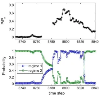
(8) As an example, Fig. 1 illustrates the filtered probabilities of the cur-rent regime along with the power output time series for a short window time. It can be seen how the filtered probabilities balance depending on the level of fluctuations. During periods with miss-ing-data, the transition matrix determines a smooth exponential convergence to the so-called ergodic probabilities (the probabilities of being in a certain regime at an arbitrary date).MSAR models can be formulated in two different ways [39]: the Intercept-Form (MSAR-IF, Eq. (9)) and the Mean Adjusted Form (MSAR-MAF, Eq. (10)). JtJF — °0
E<
l(St) yt-i e(*)3 ^ - ^ E ^ - *-.-/4
s
c(*)
(9) (10) 8740 8760 8780 8800 8820 8840 8740 8760 8780 8800 time step 8820 8840Fig. 1. Filtered probabilities of the current regime provided by the MSAR model during periods with missing data. PjPN represents the output power (P) normalized with the rated power of the wind farm (PN).
2.3. TARSO models
Open loop threshold autoregressive models are a kind of re-gime-switching model where the current regime st is assessed by
a predefined function of the available observations of exogenous variables, st =st(Aft_i). Hence the process is called observable. Usu-ally, only a certain lag of xt is considered, st = g{xt_iag). In that case,
regimes are settled by a certain number of thresholds, /0, l\, l2 lr,
that divide the space spanned by {xt} in r subsets, called S,-,
j = 1 r from now. Then, xt_tag e S¡ <s> /,•_-[ < xt_tag < l¡.
In this article only the previous lag of the exogenous variable is considered in assessing regimes. An AR process is assumed in each regime. For the sake of simplicity, all the AR processes will have the same order p. The model is given by:
y
t= 0
oSt)+ E
ef
t )^ - . ' +
£¡
.w
( i i )st= <
xt-i e Si
xt-i e S2 xt-i e Sr
With the mentioned hypothesis, the implementation of a TARSO model gives rise to three questions: (i) what is the number, r, of re-gimes considered, (ii) what is the optimal value for the set of thresholds 1 = {/0 lr} and (iii) what AR order p to choose.
Modelling a wind power time series with the described TARSO model implies that the wind farm output has clearly differentiated dynamics depending on the value of some observed variable. For example, in the case of the wind direction (wd), a different behav-iour of the wind power time series would be expected depending on the local wind direction observed at the moment of making the forecasting, wdt^. If wdt_! crosses one of the thresholds given by 1, then there is an abrupt change on the AR process that provides the forecast yt.
2.4. CPARX models
When no regimes are considered, both forms are equivalent by con-sidering 4>i = 8i, Vi>0 and fiQ = 0O/(1 - SXie0- Nevertheless, MSAR-IF and MSAR-MAF model different underlying dynamics [39].
Conditional parametric models are characterized by a smooth dependence of their coefficients with a certain variable. In particular, the CPARX models generalize an AR model by letting
the coefficients depend on available observations of exogenous variables, 0¡ = 8¡(Xt-i). As in the preceding case, only the previous
lag of the exogenous variable will be considered. The model is gi-ven by:
yt = 0o(xt-i) + J2 e>(xt-i) -yt-i + £t (12) A central point is how to define the coefficient-functions 6,{xt--i).
They can be estimated with non-parametric techniques from histor-ical data or by means of a parametric function [40,41]. In this work, the latter case will be considered.
Modelling a wind power time series with a CPARX model im-plies that the wind farm output dynamic is expected to change smoothly depending on the value of some observed variable xt_i.
For example, in the case of the wind speed, (ws), the observed local value wst_i fixes at each time step the AR process (through the
coefficient-functions ©¡(ws,^)) that provides the forecast yt. 3. Description of the data
The data considered originates from the offshore wind farm lo-cated at Horns Rev, off the west coast of Denmark. This wind farm has a rated power of 160 MW. Measurements of wind power output, wind speed and direction are available for each wind turbine, with a 1-s sample rate. 10-min resolution time series are derived by aver-aging raw data. At least 75% of the data within an interval has to be considered as valid in order to consider the averaged value also valid. The averaging process assures that the fast fluctuations related to the turbulent nature of the wind have been filtered. The period considered ranges from 16th February 2005 to 31st January 2006, consisting of 50,400 data points with 8790 missing data. The data-base has been divided into the following 3 sets:
• Training-set, from 16th February to 31st May 2005: the param-eters of the models are estimated considering this data set by solving the minimisation problem given by Eq. (3).
• Validation-set, from 1st June to 31st August 2005: the forecasts provided by the trained models are evaluated during this sec-ond period. By doing this, it is possible to assess the generaliza-tion capabilities of each model, which means that a certain model trained over a first period keeps its prediction perfor-mances over a different time period.
• Test-set, from 1st September 2005 to 31st January 2006: a benchmark analysis between validated models is carried out based on their forecasting performance in this period.
It should be notice that the division of the data-set does not per-mit models to capture seasonalities during the training process, which covers almost 4 months. This seasonalities are expected to be present in wind power time series considering the seasonal var-iability of wind at Horns Rev observed in Vincent et al. [42]. How-ever, it does not necessarily imply that the optimal models would dramatically change from 1 month to another. In any case, the optimisation of the models taking into account seasonal variations would require several years of data (not available for this work) and the implementation of models with time-varying parameters being adaptively estimated. In this regard, the implementation of adaptive MSAR models was addressed in [30].
4. Application of the models
In this section, the implementation of the models considered in Section 2 in the case of data described in Section 3 is presented. The section is divided in four subsection on different alternatives about the explanatory variables considered. Each model is trained
with different structures (concerning for example the AR order and the definition of regimes). The optimal parametrisation of each model was chosen regarding the generalisation capabilities across the validation-set. The performance of the models is evaluated in terms of the Normalized Root Mean Square Error (NRMSE) and the percentage of Improvement Over Persistence (IoP), defined as follows: NRMSE = J - • "N IoP{%) = 100
E
N t=p+l NRMSEQ -<yt-yty N-p •NRMSE NRMSE, (13) (14) where PN is the rated power of the wind farm and NRMSE0 is theNRMSE obtained with Persistence . Both criteria are suggested in
Madsenet al. [37], which includes a broad overview of ways to eval-uate wind power prediction methods.
4.1. Reference models
This subsection deals with the implementation of the reference models described in Subsection 2.1 (Persistence and linear AR) and Subsection 2.2 (MSAR models). As previously mentioned, Persis-tence does not have free parameters to be estimated. Thus, the per-formance of this model is evaluated in a straightforward way. This is not the case for the linear AR models, since the appropriate AR order p and the set of parameters 0AM¿>) need to be estimated. For a given value of p, &AR(P) is estimated by means of the
Yule-Walker equations (available in several works, e.g. [43]) over the training period. Then, the evaluation of the trained models over the validation-set allowed the optimal value of p = 3 to be identified.
Next, both MSAR-IF and MSAR-MAF architectures are employed to model the wind power time series of Horns Rev. In order to esti-mate 0MSAR, the Expectation-Maximization algorithm introduced in Dempster et al. [44] and further described in Hamilton [45] is ap-plied (for further details, see [38,46]). In the case of the MSAR-IF form, three regimes were identified with the following set of parameters: Regime st- l St-2 St-3 P = "0.77 0.11 0.27 0O 0.01 0.04 0.00 0.02 0.21" 0.73 0.16 0.03 0.70 0i 1.24 1.21 1.45 02 - 0 . 4 7 - 0 . 2 4 - 0 . 5 0 03 0.19 0.00 0.04 a 0.0573 0.0004 0.0075
On the other hand, the MSAR-MAF model identified the two follow-ing regimes: Regime st- l St-2 P = 0.91 0.07 Ho 0.52 0.53 0.09 0.93
<h
1.25 1.38 4>2 - 0 . 4 6 - 0 . 4 5 4>3 0.18 0.08 a 0.0565 0.0121In both cases, the regimes were identified by sorting different levels of fluctuations, i.e., different values for o"(l), the standard deviation of the noise.
4.2. Modelling the influence of the local wind direction
In this subsection, the inclusion of the local wind direction into both TARSO and CPARX models is detailed. In order to get some clues about the dependence of wind power on wind direction, a preliminary analysis has been carried out. This would eventually suggest restrictions to the design of appropriate varying-coefficient models, e.g. the number of regimes and the shape of the parameter functions. Then, both the TARSO(wd) model and the CPARX(wd) model are implemented.
4.2.1. Preliminary analysis
The central idea is to train a linear AR model over a subset of the training data. The subset is given by the membership of the previ-ous wind direction lag to a certain sector over the wind rose. The set of AR coefficients, 0AR, and the NRMSE obtained characterize
the dynamic of the wind power output related to this particular sector. Then, by sliding smoothly the orientation of the sector and repeating the process, one observes the impact of wind direc-tion on wind power dynamics.
Let us consider a main direction a0 and a sector width h. The
AR(p) model for this sector is given by:
{ Vt: wdt_i e a0 ± h/2
The estimation of this model provides specific values for &AR(P) and
NRMSE, related to a0. Fig. 2 illustrates the dependence of a0 on
&AR(P) and the NRMSE, when considering the case for p = 2 and
h = 90°. The following conclusions were derived from the previous analysis, where the considered values forp ranged from 1 to 5: (i) AR coefficients showed a certain dependence on a0 for any value
of p. This dependence is smooth sinus-shaped, (ii) The highest
NRMSE (thus, the lowest predictability) is related to 270-310°
direc-tions, (iii) The relationship between the NRMSE and a0 shows a
sim-ilar tendency in both the training-set and the validation-set. Hence, the influence of the wind direction learnt from historical data seems to be representative enough to model future behaviour.
4.2.2. TARSO models based on a wind direction criterion: TARSO(wd)
The previous analysis highlights different predictability levels, depending on the wind direction. Furthermore, there seems to be a high predictability orientation (E-SE), a low one (W-NW) and intermediate transitions. This fact suggests a low number of re-gimes to be considered a priori.
The TARSO model was introduced in Eq. (11). In this particular case, regime thresholds 1 will be related to wind direction sectors as follows: let us consider a main direction a0 and a certain width
1.5 a:
<
-0.5 90 180 270 360 0 90 180 270 360%n
sector h. For the sake of simplicity, the same h will be considered for every sector. The wind rose can be split in r = 360°/h sectors (the considered widths in the preliminary analysis assures that the number of sectors is a natural number between 2 and 8) by defining the following thresholds:
Í 0 = í r
2 / - 1
h, j = 1 , . . . , r
This procedure provides the definition of 1 and r, given values of a0
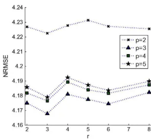
and h. Once the sectors have been defined, AR coefficients can be estimated for each regime once more by means of the Yule-Walker equations. Fig. 3 shows the NRMSE obtained in the validation-set as a function of p and r, when considering the optimal orientation a0
obtained. It can be noted that the model with the best generaliza-tion capability was obtained for the case of p = 3. In the same way, it does not seem to be worth increasing the number of regimes further than 3. In relation to the orientation sectors, Fig. 4 illustrates the best ones for the six AR(3) models. It can be seen that the sec-tors are placed in such a way that the above mentioned low predict-ability orientation (W-NW) tends to form an independent regime, independently of the number of regimes considered.
The TARSO(wd) model that showed the best performance in the validation-set was: yt = ( 0.00 + 1.36 yt_!
J 0.01 +1.40 y
t_!
( 0.00 +1.19 y ^ j - 0 . 5 1 -yt_2+ 0.14 .yt_3, - 0.54 -yt_2+ 0.13 -yt_3, - 0.43 -yt_2+ 0.23 .yt_3, st = l St = 2 st = 3 The regimes were given by:Í 1 , w dM e [-41°, 79°) st = i 2, wdt-i € [79°, 199°)
( 3 , wdt-i € [199°,319°)
4.2.3. CPARX models based on a wind direction criterion: CPARX(wd)
The description of CPARX models in Subsection 2.4 highlights that the crucial point is how to define the coefficients as a function of a certain exogenous variable. Considering the previous prelimin-ary analysis, a sinus-shaped dependence is proposed:
LU a: 4.24 4.23 4.22 4.21 4.2 4.19 4.18 4.17 4.16 x x ,.x x " ' X ' ' ' • ••»•• p = 2 • • A . . p = 3 •••D" p=4 ' • • ' • p = 5
.•.., .
éf ' • • . . * • •»..."•....
-y
A„„ »••"
A< " ' * / ' *
'"'•A"'Fig. 2. Dependence of the AR coefficients (left) and NRMSE in %PN (right) with local wind direction. Case for AR order p = 2.
Fig. 3. NRMSE (in %PN) of TARSO(wd) over the validation-set, as a function of the
number of regimes, r, and the AR order, p. Results for p = 1, layout of the picture due to a higher NRMSE.
Fig. 4. Optimal orientation of the sectors depending on the number of regimes considered in a TARSO(wd) model, case for AR order p = 3.
y
t= 0o(wd
t_i) + J2
ed
wdt-i) -y
t-i
¡=i
0,-(wdt_i) = a¡ + bi • cos(wdt_i - <¿>0), i = 0 , . . . ,p
(15) (16) a, being the mean level of the ¡th AR coefficient and b¡ being the amplitude of the dependence of 0,- on the wind direction. Then, for a given value of p, the set of parameters is formed by:
0c {a0,...,av,b0,...,bv,<j)0} (17)
&CPARX is estimated in accordance with Eq. (3). As in the previous
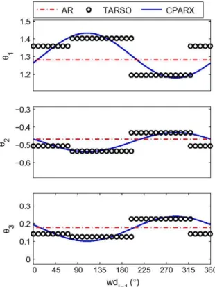
case, the best performance in the validation-set was achieved for the case of p = 3. Fig. 5 collects the AR coefficients for the AR model, the TARSO(wd) model and the CPARX(wd) model.
4.3. Modelling the influence of the local wind speed
Following a similar methodology, this subsection focuses on how the local wind speed can be used to define regimes or smooth dependences in the wind power time series dynamics. A prelimin-ary analysis between the predicted variable and the wind speed is firstly performed. Then, the TARSO(ws) model and the CPARX(ws) model are obtained.
4.3.1. Preliminary analysis
Let us consider the interval of wind speeds / = [ws0 - h\
2,ws0 + f¡/2). An AR(p) model is trained taking into account only those data that satisfy at time t the condition wst^ e I. For a certain
h, the AR coefficients and the NRMSE obtained are related to the
wind speed ws0. Then, the interval / slides over the spanned space
of the wind speed in order to reveal how the time series dynamic and the predictability vary with ws0. The following conclusions
were obtained, where the considered values for p ranged from 1 to 5: (i) The AR coefficients show a certain dependence on the wind speed. This dependence is close to be linear in a substantial part of the wind speed range, as is shown in the Fig. 6 (case p = 2, h = 4 m/ s). (ii) The NRMSE tends to be higher for high wind speeds, showing a maximum at a wind speed of around 10-12 m/s. However, a de-crease in the NRMSE is observed for wind speeds beyond the nom-inal wind speed (at which the output power is constant up to the
1.5 1.4 CD~ 1.3 1 2 A R
y**o
o
oooc TARSO feGQOOOO U r A K X OOOOO 135 180 225 270 315 360 w dM (°)Fig. 5. Dependence of the AR coefficients with local wind direction for AR, TARSO(wd) and CPARX(wd) models (00 is omitted, since it is very close to zero for every model).
cut-off wind speed), (iii) A similar tendency of the relationship be-tween NRMSE and wind speed has been found for both the train-ing-set and the validation-set (see Fig. 6). This fact suggests that the data sets are representative enough to consider this informa-tion valid for future time periods.
4.3.2. TARSO models based on a wind speed criterion: TARSO(ws)
The prior analysis reveals that a regime-switching model can be implemented in order to catch different predictability levels, though a low regimes number is suggested from Fig. 6. In this case, the optimisation process considers the threshold values, 1, as parameters to be estimated. Then, for a certain number of regimes, r, and the AR order p, the set of parameters to estimate is given by:
0T, <0 AR'»' , 0 AR,r
,1)
(18) 2 1.5 1 0.5 0 -0.5 LUa.
! \ : • train validation,
5 10 ws (m/s) 15 5 10 ws (m/s) 15Fig. 6. Dependence of the AR coefficients and NRMSE (in %PN) with local wind speed. Case for AR order p = 2.
6'TARSO is estimated by means of a numerical algorithm based on the
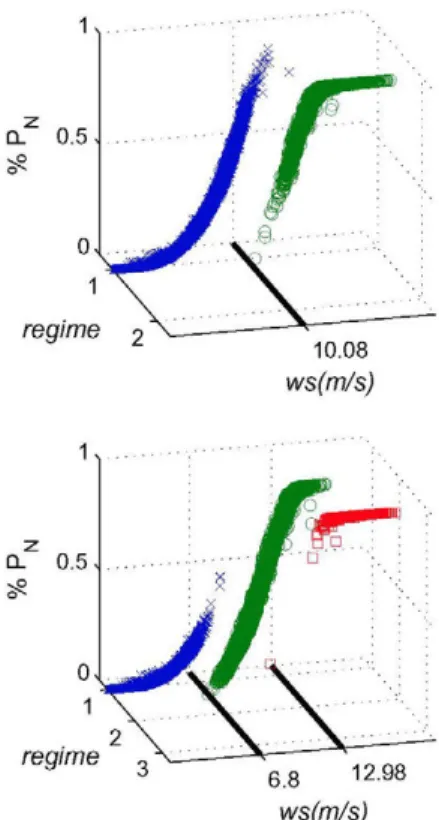
criterion given by Eq. (3). Two and three regimes have been pro-posed with AR orders going from 1 to 5. In all the cases, the AR(3) showed the best performance in the validation-set (see Fig. 7). Fur-thermore, the two-regimes model was slightly better than the three-regimes one. Fig. 8 illustrates the power curve depicted under the optimised regimes. In both cases, the thresholds obtained seems to be related to the shape of the power curve. First, considering two regimes lead to a threshold of around 10 m/s near the inflexion point. This value splits up the power curve in two regions: (i) the first one is characterized by a convex relationship between the wind speed and the output power. In an ideal case, this relationship is a cubic polynomial given by P = \pCpAv3', where p is the density of
air, Cp is the power coefficient, A is the area swept by the rotor
blades and v is the wind speed, (ii) The second part is characterized by a concave relationship, since the output power has to be limited by the rated power of the wind turbine. On the other hand, consid-ering three regimes leads to a division clearly based on the slope of the power curve: two regimes for the two flat regions (for low and high wind speeds) and a third one for the steep part.
The TARSO(ws) model with best generalisation capabilities was:
yt =
' 0.00 + 1.33 -yt_t - 0.50 -yt_2 + 0.18 -yt_3, st = 1
k - 0 . 0 2 + 1.22 • yt_-¡ - 0.39 • yt_2 + 0 . 1 8 - yt_3, st = 2
The regimes w e r e given by: 1, w sM < 10.08 2, wst^ > 10.08 st a. 0.5. regime 2 0.5. 10.08 ws(m/s) regime 6.8 12.98 ws(m/s)
Fig. 8. Optimal splitting of the power curve for TARSO(ws) models.
4.3.3. CPARX models based on a wind speed criterion: CPARX(ws)
In this case, a linear dependence between AR coefficients and the last available data of wind speed wst^ is proposed (Eqs. (19)
and (20)). This is partially supported by the preliminary analysis: even though this hypothesis does not seem to be accurate for low and high wind speeds, Fig. 6 reveals that it is the case for a sub-stantial part of the wind speed range.
yt = 0o(w st-i) + j]0¡(wst_i) -yt_i ¡=i
0¡ (wst_i) = a¡ + bi • (wst-i), i = 0 , . .
(19) (20)
a¡ being t h e ¡th AR coefficient a t null w i n d speed a n d £>, being t h e
slope of t h e d e p e n d e n c e of 0, on t h e w i n d speed. The set of p a r a m -eters is n o w given b y 0CPARX = {c¡o <%>, b0 bp} a n d e s t i m a t e d in
accordance w i t h Eq. (3). The minimisation process has b e e n carried out for several AR orders, p = 1, 2 5, giving p = 3 t h e optimal
value in t e r m s of generalisation capabilities. Fig. 9 collects t h e AR coefficients obtained as a function of t h e w i n d speed for t h e AR model, t h e TARSO(ws) model a n d t h e CPARX(ws) model.
4.4. Combining both effects: CPARX(wd,ws)
Results concerning the incorporation of local wind direction and local wind speed in varying-coefficient models will be discussed in Section 5. However, at this point, it is worth noting that CPARX models showed a better performance than TARSO models when modelling the effect of the considered explanatory variable (see Fig. 11). Additionally, each exogenous variable seems to provide information about different effects. In base of this hypothesis, the following CPARX model considering both wind speed and wind direction is proposed: yt = 0o(w dt - i , w s ^ ) + J20i(wdt_!,wdt_!) -yt_¡ (21) 4.36 LU w a: 4.34 4.32 4.3 4.28 4.26 4.24 4.22 4.2 £
V,
'•••'• -•A- 2 regimes " • • " 3 regimes D ...A 2 3 4 5 PFig. 7. NRMSE (in %PN) of TARSO(ws) over the validation-set, as a function of the number of regimes, r, and the AR order, p.
di(wdt_i,wst_i) = ai + bi •cos(wdt_1 - <¡>0) + c¡ • (wst_i),i
= 0 , . . . , p (22) The set of p a r a m e t e r s t o b e e s t i m a t e d is &CPARX = {C¡O <%>,
£>o bp, c0 cp, 4>oi- In this case, t h e best model obtained w a s
for a n AR order of p = 4. The coefficient-functions ^ ¡ ( w d t ^ . w s t ^ ) are n o w surfaces t h a t replicates t h e same trends found in t h e pre-vious sections. As a n example, t h e case oí 8^ is illustrated in Fig. 10. 5. Results
This section gathers the results obtained over the test-set, when the optimal parametrisation of each model obtained in Section 4 is considered.
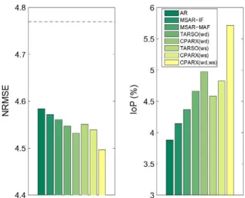
Globally, the improvements over Persistence ranged from al-most 4% to more than 5.5% (see Fig. 11). This represents a good per-formance, since Persistence is traditionally difficult to improve on
AR ° TARSO CPARX
5 10
wst1 (m/s)
Fig. 9. Dependence of the AR coefficients for AR, TARSO(ws) and CPARX(ws) models.
(6>o is omitted, since it is very close to zero for every model).
2-, 1.75- 1.5-J- 1.251 - 0.75-0
\
v __----" < 1 0 ^ WS •¡(m/s) 360 20 0Fig. 10. 6i as a function of local wind direction and local wind speed for the
CPARX(wd,ws) model.
for a prediction horizon of 10 min. With regard to the reference models and in accordance with the previous studies [29,30], improvements in very-short term point-forecasting can be at-tained when considering several regimes under the absence of other explanatory variables. In particular, MSAR models were able to capture shifts between non-observed meteorological states, delivering information about wind power fluctuations and provid-ing a better performance than Persistence and linear AR models.
The models taking into account exogenous variables overcome the reference models. Regarding the influence of the local wind direction, a similar relationship between this variable and the AR parameters was identified by the TARSO(wd) and the CPARX(wd) models, as shown in Fig. 5. In particular, given that Persistence can be considered as a particular case of AR model with 0^ = 1
4.8 r 4.7 5.5 LU a: Q_o 4.5 3.5 ] A R 1MSAR-IF 1MSAR-MAF I TARSO(wd) I CPARX(wd) I TARSO(ws) | CPARX(ws) ]CPARX(wd,ws;
Fig. 11. NRMSE (in %PN) and IoP for the test-set. Dashed line of the figure on the left refers to the NRMSE of persistence.
and 0¡ = O, V i > l , both TARSO(wd) and CPARX(wd) models were likely to become globally closer to Persistence for wind directions related to the W-NW sector, characterized by a low predictability (the only exception being <93, which experiences a small increment for the mentioned wind directions). Additionally, a smooth depen-dence of the wind power dynamics on the local wind direction was found to be preferable to considering different regimes (though special attention was paid to track the optimal number of sectors and their orientation) given the IoP of 4.98% and 4.66% respectively. Similar conclusions were obtained when the local wind speed was considered as an exogenous variable: both models TARSO(ws) and CPARX(ws) became globally closer to Persistence (with the only exception of 03, which remains almost constant) for high wind speeds (Fig. 9) characterized by a lower predictability, and a smooth dependence of the coefficient-functions on the wind speed provided a better result than the regime-switching strategy (an IoP of 4.82% compared to 4.58%).
In general, the models that took into account the wind direction attained slightly better results that those including the wind speed. This was also found when considering the results depicted monthly (Tables 2 and 3), the only exception being the month of January. However, in both a globally and a monthly basis, the best performance was clearly attained by the CPARX(wd.ws). This mod-el attained a global IoP of 5.72%, which represents almost the addi-tion of the single improvements obtained by the CPARX(wd) and the CPARX(ws) models with respect to the AR model. This finding is particularly significant as it supports the notion that each explanatory variable gives information about effects of a different nature.
Table 2
NRMSE depicted monthly. The two lowest values in each column are given in bold fonts. The overall results are gathered in Fig. 11.
Persistence AR MSAR-IF MSAR-MAF TARSO( wd) CPARX( wd) TARSO( ws) CPARX( ws) CPARX( wd,ws) September 4.66 4.44 4.43 4.41 4.42 4.41 4.44 4.42 4.41 October 4.16 3.96 3.95 3.96 3.92 3.92 3.93 3.94 3.91 November 6.25 6.03 5.97 5.95 5.94 5.91 5.94 5.92 5.82 December 4.76 4.42 4.47 4.41 4.37 4.37 4.39 4.37 4.35 January 4.07 3.98 3.97 4.00 3.99 3.97 3.97 3.94 3.93
Table 3
IoP depicted monthly. The two highest values in each column are given in bold fonts. The overall results are gathered in Fig. 11.
September October November December January
AR MSAR-IF MSAR-MAF TARSO( wd) CPARX( wd) TARSO( ws) CPARX( ws) CPARX(wd,ws) 4.73 4.74 5.30 5.07 5.34 4.72 5.07 5.37 4.89 5.04 4.81 5.72 5.71 5.65 5.39 5.96 3.54 4.43 4.80 4.87 5.41 4.89 5.16 6.78 7.19 6.10 7.46 8.17 8.34 7.89 8.14 8.68 2.33 2.50 1.80 2.07 2.54 2.57 3.30 3.54 5.1. Further discussion
It was found that the incorporation of the wind direction as an explanatory variable leads to an appreciable improvement of the prediction performance. It could be due to the fact that the pro-posed models managed to capture some influence of the local wind direction on the wind power time series dynamics. Vincent et al. [42] related the influence of the wind direction on the wind vari-ability at Horns Rev to synoptic scale forcings combined with the location of the wind farm with respect to the shore. In particular, a high wind variability was observed for Westerly winds. Accord-ing to Akhmatov et al. [47], the implementation of the models of Subsection 4.2 evidences that these effects are propagated to the wind power time series. As mentioned above, it is interesting to note that a smooth dependence of the wind power dynamics on the local wind direction was preferable to a regime switching strat-egy. This could be explained by taking the following consider-ations: the present study is focused on an offshore wind farm, characterized by a flat topography with a uniform-clustered distri-bution of the wind turbines over a squared area. Hence, for this wind farm configuration no obstacle is introducing directional aerodynamic disturbances and, additionally, wind turbine wakes are likely to have a weaker impact on the dependence between the wind power and the local wind direction compared to the case of a single row wind farm configuration. Even though some works [10,11] suggest a considerable influence of the wakes for very nar-row sectors around the wind turbines line direction, this seems to be too specific to be relevant from a statistical point of view (at least with the models considered in this work). Our results suggest that the influence of the local wind direction on the wind power dynamics was likely to be related to synoptic conditions rather than microscale effects. However, microscale effect could become predominant in other study cases. Modelling the influence of the local wind direction in wind farms located in complex terrain, where topographic obstacles and non-homogeneity of the terrain introduce strong directional dependences on the power produc-tion, could require other AR coefficient-functions, instead of the sinus-shaped ones proposed here. Furthermore, wind farms with a non-squared distribution of wind turbines, for instance row-configured wind farms, could even require a regime switching strategy, since the wind turbine wakes would affect dramatically the performance of the wind farm for certain wind directions. In any case, further research on complex terrain and different config-uration of wind farms would be required for confirmation.
On the other hand, when the local wind speed was considered as an exogenous variable, the optimisation of the models were likely to be related to the characteristics of the non-linear power transformation process. Considering that the power curve repre-sents a non-linear transformation from wind speed to wind power, the slope of this curve provokes an amplification/reduction effect of the wind speed fluctuations. It has a direct impact on the output power dynamics, causing a dependence between the wind speed and the predictability of the output wind power. Hence, the
improvement obtained could be due to the fact that the wind speed was employed as a signal about this non-linear effect. The regime-switching strategy provided thresholds of wind speed that divide the power curve into particular parts (convex-concave for the case of 2 regimes and low-high-low amplification level for the case of 3 regimes, see Fig. 8). For the case of the conditional parametric model, a linear relationship between the AR coefficients and the wind speed seemed to be appropriate for a greater part of the wind speed range. However, the saturation effect of the output power related to extreme wind speeds (close to zero or above the nominal wind speed) has not been addressed. Future work could deal with this topic by considering the Generalized Logit transfor-mation described in Pinson and Madsen [48] or the so-called 'break-point models', a special subclass of varying-coefficient mod-els that combine both CPARX and TARSO modmod-els (see the closing discussion in Hastie and Tibshirani [49]).
6. Conclusions
We have presented a study focused on modelling the influence of local wind speed and direction on the dynamics of a wind power time series. With this purpose, a benchmark between several vary-ing-coefficient models for 10 min-ahead forecasting was carried out. The models are built by generalising the conventional linear AR structure, following two approaches: regime switching models and conditional parametric models. By comparing the accuracy of the models, findings about the most suitable statistical approach were also obtained.
It was found that local measurements of both wind speed and direction provide useful information for a better comprehension of the wind power time series dynamics, at least when consider-ing the case of the very-short term forecastconsider-ing. In particular, the results suggest that different effects can be modelled depending on the considered explanatory variable: the local wind direction contributes to model some features of the prevailing winds, such as the impact of the wind direction on the wind variability, whereas the non-linearities related to the power transformation process can be introduced by considering the local wind speed. Additionally, for our particular case study, it was found that the conditional parametric models outperforms a regime-switching strategy.
It is interesting to note that the influence of both local wind speed and direction were modelled under the assumption of ob-servable processes, and that only the last observation was taken into account. This study highlights two main lines for further re-search: the first one is to consider non-observable processes based on local observations, by incorporating exogenous vari-ables whether in the transition matrix or in the definition of the AR coefficients of MSAR models. The second one is to include previous lags of the local observations in order to get a model sensitive to the evolution of the considered exogenous variable. By doing this, it would be possible to explore new effects that condition the dynamics of the output wind power time series (e.g. abrupt changes in local wind direction related to certain meteorological conditions).
Finally, the models here presented could be upgraded by letting the coefficients vary smoothly with time so as to capture seasonal variabilities of wind power dynamics due to climatological effects and the decrease of the wind turbine performance.
Acknowledgements
Acknowledgements are first due to CIEMAT who is founding the research of the first author through its Ph.D Scholarship Program. The work presented has also been partly supported by the Danish
ForskEL programme through the Project "Radar@Sea" (ForskEL 2009-1-0226) and the project "Mesoscale atmospheric variability and the variation of wind and production for offshore wind farms", sponsored by the Danish Public Service Obligation (PSO) fund (PSO 7141), which are hereby acknowledged. We are thankful to Vatten-fall Denmark for originally providing the wind and power measurements for the Horns Rev wind farm, and to Pierre-Julien Trombe for the data processing and quality checking.
Purvins A, Zubaryeva A, Llórente M, Tzimas E, Mercier A Challenges and options for a large wind power uptake by the European electricity system. Appl Energy 2011;88(5):1461-9.
Snyder B, Kaiser MJ. A comparison of offshore wind power development in europe and the US: Patterns and drivers of development. Appl Energy 2009;86(10):1845-56.
Giebel G. The state of the art in short-term prediction of wind power - a literature overview. Tech. Rep.; ANEMOS EU project; 2003.
Landberg L, Giebel G, Nielsen H, Nielsen T, Madsen H. Shortterm prediction -an overview. Wind Energy 2003;6(3):273-80.
Costa A, Crespo A, Navarro J, Lizcano G, Madsen H, Feitosa E. A review on the young history of the wind power short-term prediction. Renew Sustain Energy Rev2008;12(6):1725-44.
Pinson P, Nielsen H, Madsen H, Kariniotakis G. Skill forecasting from ensemble predictions of wind power. Appl Energy 2009;86(7-8):1326-34.
Bouzgou H, Benoudjit N. Multiple architecture system for wind speed prediction. Appl Energy 2011;88(7):2463-71.
Costa A. Mathematical/statistical and physical/meteorological models for short-term prediction of wind farms output. Ph.D. thesis. Escuela TTcnica Superior de Ingenieros Industriales (Universidad PolitTcnica de Madrid); 2005. Orlanski I. A rational subdivision of scales for atmospheric processes. Bull Am Meteorol Soc 1975;56:527-30.
Jensen L, Morch C, Sorensen PB, Svendsen KH. Wake measurements from the Horns Rev off-shore wind farm. European Wind Energy Conference, London; 2004.
MTchali M, Barthelmie R, Frandsen S, Jensen L, RTthorT PE. Wake effects at Horns Rev and their influence on energy production. European Wind Energy Conference, Greece; 2006.
Brown B, Katz R, Murphy A. Time series models to simulate and forecast wind speed and wind power. J Clim Appl Meteorol 1984;23(8):1184-95. Huang Z, Chalabi ZS. Use of time-series analysis to model and forecast wind speed. J Wind Eng Ind Aerodynam 1995;56(2-3):311-22.
Kennedy S, Rogers P. A probabilistic model for simulating long-term wind-power output. Wind Eng 2003;27(3):167-81.
Torres J, Garcia A, De Blas M, De Francisco A. Forecast of hourly average wind speed with ARMA models in Navarre (Spain). Solar Energy 2005;79(l):65-77. De Giorgi MG, Ficarella A, Tarantino M. Error analysis of short term wind power prediction models. Appl Energy 2011;88(4):1298-311.
Erdem E, Shi J. ARMA based approaches for forecasting the tuple of wind speed and direction. Appl Energy 2011;88(4):1405-14.
Liu H, Erdem E, Shi J. Comprehensive evaluation of ARMA-GARCH (-M) approaches for modeling the mean and volatility of wind speed. Appl Energy 2011;88(3):724-32.
Li G, Shi J. On comparing three artificial neural networks for wind speed forecasting. Appl Energy 2010;87(7):2313-20.
Cleveland WS, Grosse E, Shyu WM. Statistical models in S; chap. Local regression models. Boca Raton, FL, USA: CRC Press, Inc.; 1991. p. 309-76. ISBN:0412052911.
Tong H. Threshold models in non-linear time series analysis. Springer-Verlag; 1983.
Gneiting T, Larson K, Westrick K, Genton MG, Aldrich E. Calibrated probabilistic forecasting at the stateline wind energy center: the regime-switching space-time method. J Am Stat Assoc 2006;101(475):968-79. Tastu J, Pinson P, Kotwa E, Madsen H, Nielsen HA. Spatio-temporal modelling of short-term wind power prediction errors. Wind Energy 2011;14(l):43-60. Hering AS, Genton MG. Powering up with space-time wind forecasting. J Am Stat Assoc 2010;105(489):92-104.
Castino F, Festa R, Ratto C. Stochastic modelling of wind velocities time series. J Wind Eng Ind Aerodynam 1998;74-76:141-51. 2nd European and African Conference on Wind Engineering, Genoa, Italy, Jun 22-26,1997.
Hughes JP, Guttorp P, Charles SP. A non-homogeneous Hidden Markov model for precipitation occurrence. J Roy Stat Soc Series C 1999;48(l):15-30. Ailliot P. ModFles autorTgressifs a changements de rTgimes markoviens. Applications aux sTries temporelles de vent. Ph.D. thesis. University of Rennes; 2004.
Kosater P, Mosler K. Can Markov regime-switching models improve power-price forecasts? Evidence from German daily power power-prices. Appl Energy 2006;83(9):943-58.
Pinson P, Christensen LEA, Madsen H, Sorensen PE, Donovan MH, Jensen LE. Regime-switching modelling of the fluctuations of offshore wind generation. J Wind Eng Ind Aerodynam 2008;96(12):2327-47.
Pinson P, Madsen H. Adaptive modeling and forecasting of wind power fluctuations with Markov-switching autoregressive models. J Forecasting; in press. doi:10.1002/for.H94.
Chen R, Tsay RS. Functional-coefficient autoregressive models. J Am Stat Assoc 1993;88(421):298-308.
Nielsen HA, Nielsen TS, Joensen AK, Madsen H, Hoist J. Tracking time-varying-coefficient functions. IntJ Adaptive Control Signal Process 2000;14(8):813-28. Sánchez I. Short-term prediction of wind energy production. Int J Forecasting 2006;22(l):43-56.
Fan J, Zhang W. Statistical methods with varying-coefficient models. Stat Interface 2008;1:179-95.
Cleveland WS, Devlin SJ. Locally-weighted regression: an approach to regression analysis by local fitting. J Am Stat Assoc 1988;83:596-610. Nielsen T, Madsen H, Nielsen H. Prediction of wind power using time-varying coefficient-functions. In: Proceedings of the 15th IFAC world congress on automatic control, Barcelona, Spain; 2002.
Madsen H, Pinson P, Kariniotakis G, Nielsen HA, Nielsen ST. Standardizing the performance evaluation of short-term wind power prediction models. Wind Eng 2005;29(6):475-89.
Hamilton JD. A new approach to the economic analysis of nonstationary time series and the business cycle. Econometrica 1989;57(2):357-84.
KrolzigHM. Markov-switching vector autoregressions. Springer; 1997. Nielsen HA, Nielsen TS, Madsen H. ARX-models with parameter variations estimated by local fitting. In: Sawaragi Y, Sagara S, editors. 11th IFAC symposium on system identification, vol. 2; 1997. p. 475-80.
Madsen H, Hoist J. Modelling non-linear and non-stationary time series. Technical University of Denmark, DTU Informatics; 2000.
Vincent CL, Pinson P, Giebel G. Wind fluctuations over the North Sea. Int J Climatol; in press. doi:10.1002/joc.2175.
Peña D. Estadística. Modelos y mTtodos, vol. 2. 2nd ed. Alianza Editorial; 1987. Dempster AP, Laird NM, Rubin DB. Maximum likelihood from incomplete data via the EM algorithm. J Roy Stat Soc Series B 1977;39(l):l-38.
Hamilton JD. Analysis of time series subject to changes in regime. J Econom 1990;45(l-2):39-70.
Patterson DM. Nonlinear time series analysis of economic and financial data. Kluwer Academic; 1999. p. 33-43. [chapter A markov switching cookbook].
Akhmatov V. Influence of wind direction on intense power fluctuations in large offshore windfarms in the North Sea. Wind Eng 2007;31(l):59-64. Pinson P. On probabilistic forecasting of wind power time-series. Tech. Rep.; Technical University of Denmark, DTU Informatics; 2010.
Hastie T, Tibshirani R. Varying-coefficient models. J Roy Stat Soc, Ser B (Methodol) 1993;55(4):757-96.