Towards Unifying Grounded and Distributional Semantics Using the Words-as-Classifiers Model of Lexical Semantics

DISTRIBUTIONAL SEMANTICS USING THE

WORDS-AS-CLASSIFIERS MODEL OF LEXICAL

SEMANTICS

by Stacy Black

A thesis

submitted in partial fulfillment of the requirements for the degree of Master of Science in Computer Science

Boise State University

DEFENSE COMMITTEE AND FINAL READING APPROVALS

of the thesis submitted by

Stacy Black

Thesis Title: Towards Unifying Grounded and Distributional Semantics using the Words-as-Classifiers Model of Lexical Semantics

Date of FinalOral Examination: 24th April 2020

The following individuals read and discussed the thesis submitted by student Stacy Black,and theyevaluatedthepresentationand responsetoquestionsduringthe final oralexamination.Theyfoundthatthestudentpassedthefinaloralexamination.

Casey Kennington, Ph.D. Chair, Supervisory Committee Francesca Spezzano, Ph.D. Member, Supervisory Committee

Sole Pera, Ph.D. Member, Supervisory Committee

The final reading approval of the thesis was granted by Casey Kennington, Ph.D., Chair of the Supervisory Committee. The thesis was approved by the Graduate College.

I wish express my sincere appreciation for my advisor, Dr. Casey Kennington, for his support and guidance throughout the culmination of this thesis. I would also like to thank Daniele Moro for his valuable insight and assistance with several of aspects of this work.

Finally, I would like to thank my family, and especially my sister, for all their love and encouragement throughout my study.

Automated systems that make use of language, such as personal assistants, need some means of representing words such that 1) the representation is computable and 2) captures form and meaning. Recent advancements in the field of natural language processing have resulted in useful approaches to representing computable word mean-ings. In this thesis, I consider two such approaches: distributional embeddings and grounded models. Distributional embeddings are represented as high-dimensional vectors; words with similar meanings tend to cluster together in embedding space. Embeddings are easily learned using large amounts of text data. However, embeddings suffer from a lack of “real world” knowledge; for example, the knowledge of identifying colors or objects as they appear. In contrast to embeddings, grounded models learn a mapping between language and the physical world, such as visual information in pictures. Grounded models, however, tend to focus only on the mapping between language and the physical world and lack the knowledge that could be gained from considering abstract information found in text.

In this thesis, I evaluate wac2vec, a model that brings together grounded and distributional semantics to work towards leveraging the relative strengths of both, and use empirical analysis to explore whether wac2vec adds semantic information to traditional embeddings. Starting with the words-as-classifiers (WAC) model of grounded semantics, I use a large repository of images and the keywords that were used to retrieve those images. From the grounded model, I extract classifier

beddings from distributional word representations. I show that combining grounded embeddings with traditional embeddings results in improved performance in a visual task, demonstrating the viability of using the wac2vec model to enrich traditional embeddings, and showing that wac2vec provides important semantic information that these embeddings do not have on their own.

ABSTRACT . . . vi

LIST OF TABLES . . . xi

LIST OF FIGURES . . . xiii

LIST OF ABBREVIATIONS . . . xv

1 Introduction . . . 1

1.1 Meaning is Grounded and Distributed . . . 1

1.2 Thesis Statement . . . 3

2 Background and Related Work . . . 5

2.1 Background . . . 5

2.1.1 Concrete and Abstract Words . . . 5

2.1.2 Distributional Semantics . . . 6 2.1.3 Grounded Semantics . . . 9 2.2 Related Work . . . 11 2.2.1 Comparison of Approaches . . . 14 3 Methods . . . 16 3.1 Data . . . 16

3.1.1 Vocabulary and Datasets . . . 16

3.2 WAC . . . 22

3.3 Embedding WAC . . . 24

3.4 Training wac2vec . . . 26

4 Evaluation . . . 31

4.1 Visual Dialogue . . . 32

4.1.1 Task & Procedure . . . 33

4.1.2 Metrics . . . 34

4.1.3 Results . . . 35

4.2 Phrase Chunking . . . 36

4.2.1 Task & Procedure . . . 36

4.2.2 Metrics . . . 37

4.2.3 Results . . . 37

4.3 Named Entity Recognition . . . 38

4.3.1 Task & Procedure . . . 39

4.3.2 Metrics . . . 39

4.3.3 Results . . . 39

4.4 Word Similarity . . . 40

4.4.1 Task & Procedure . . . 41

4.4.2 Metrics . . . 41

4.4.3 Results . . . 42

4.5 Discussion of Results . . . 42

5 Conclusions . . . 45

5.1 What have we done so far? . . . 45

REFERENCES . . . 47

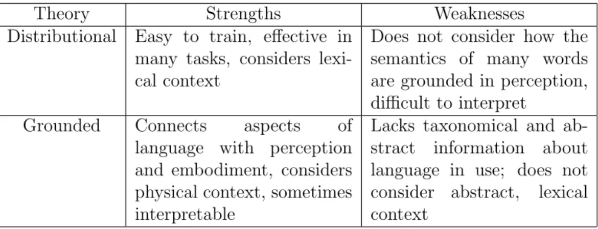
2.1 Strengths and weaknesses of distributional and grounded semantic theories. . . 6

4.1 Results from the visual dialogue task. The top half of the results are for the v0.9 dataset, and the bottom half are for the v1.0 dataset. From left to right, metrics are: mean rank; recall at 1, 5, and 10; and mean reciprocal rank. Best results are bolded. For best results that combine wac2vec and an embedding, we calculated the statistical significance using a paired t-test, with an alpha of 0.05. Our null hypothesis was that wac2vec does not improve the performance of the distributional embedding. With p-values of<0.01 for each result we tested, we found that these best-performing results were statistically significant. . . 34 4.2 Results from the chunking task. The two metrics here are F1 score

and accuracy. Starred BERT indicates BERT provided by the Flair library. Best results are bolded. . . 38 4.3 Results from the named entity recognition task. The two metrics here

are F1 score and accuracy. Starred BERT indicates BERT provided by the Flair library. Best results are bolded. . . 40

correspond to the SimLex-999 dataset, and the bottom half shows results on the WordSim-353 dataset. The metric used in this task is the Spearman correlation. Best results are bolded. . . 42

2.1 An image and accompanying referring expressions from the RefCOCO

dataset. . . 9

3.1 Correlation between word concreteness and the age that those words were learned. As can be seen, words learned at younger ages are highly concrete, and words learned at older ages are more abstract. The graph does start to trend upwards at the highest ages, especially for ages 18 and 19, though it is worth noting that for these ages, there were only 5 and 2 words, respectively, in the AoA dataset. . . 18

3.2 In this graph, words were placed into concreteness bins that increment by 0.5 (for example, (2.5, 3.0], which is a range inclusive of values of 2.5 and exclusive of values of 3.0). There is a roughly even distribution of levels of concreteness in the AoA dataset, except for the (1.0, 1.5] concreteness range, which has few words. . . 19

3.3 Google image search results for the word “red.” . . . 21

3.4 Google image search results for the word “democracy.” . . . 22

3.5 Google image search results for the word “apple.” . . . 23

collection of images described by the word red are passed as inputs in order to train a binary classifier (such as logistic regression). After training, the classifier is able to return a prediction of whether a given image belongs to the semantic class “red.” . . . 24 3.7 Clusters of classifier hidden layer coefficients, as shown in Moro et al.

[33]. The vocabulary is the top 100 words from the MSCOCO dataset. . 26 3.8 Structure of the wac2vec red classifier, which has been trained on 100

images depicting the word red. The classifier takes in an input of 1000 features, has two hidden layers of 5 nodes each, and a binary sigmoid that outputs the prediction of whether a given image belongs to the semantic class “red.” The bottom layer has 5005 coefficients (5000 weights + 5 bias terms), the upper layer has 30 coefficients (25 weights + 5 bias terms), and the final binary sigmoid has 6 coefficients (5 weights + 1 bias term). . . 27 3.9 Graph of the resulting dimensionality after reducing the wac2vec

vec-tors to difference variances. . . 28

NLP – Natural language processing

AoA– Age of Acquisition

WAC – Words-as-classifiers

CNN – Convolutional neural network

CHAPTER 1

INTRODUCTION

1.1

Meaning is Grounded and Distributed

Representing some kind of semantic approximation of language is essential in any automated task that uses natural language, including machine translation, speech transcription, and web search, among others. Though it is relatively automatic for humans to acquire the meanings of words, acquiring and representing semantic meaning in computational machines remains an unsolved challenge. Current ap-proaches to semantics do not have a holistic method of learning and representing semantics that takes into account all aspects of a word’s semantic meaning. There are several competing, yet potentially complementary approaches to semantics: formal semantics, distributional semantics, and grounded semantics. This thesis focuses on approaching a unification of the latter two: distributional, which has seen success in recent years, and grounded, which we argue provides crucial information that distributional semantics lacks. Including formal semantics is beyond the scope of this work.

In distributional semantics, the meaning of a linguistic term is based on the way that it is distributed amongst other terms. In other words, a word that occurs in a similar context as another word is likely to have similar semantic meaning. One com-mon approach to distributional semantics is to represent a word as a high-dimensional

vector, termed embeddings, such as Word2vec [32]. In contrast, grounded semantics attempts to model how the meaning of a word is based on perception of the world (e.g. visual or audio). For example, people know what red means because they have seen objects that are called red; they did not learn its semantic meaning by reading about it in a dictionary.

Both theories have their advantages: for example, distributional embeddings can be easily trained on text, and grounded models are useful in tasks that depend on perception, such as robots and self-driving cars; these advantages are discussed in more depth later in this thesis. Both also make assumptions that leave them without important aspects of meaning: grounded semantic models often assume independence of words with each other, ignoring lexical context, and distributional semantics assumes all words are distributional, and ignores the fact that the meanings of many words have some kind of anchor in the real world. Any natural language processing task that has words that are physically grounded is potentially unable to draw upon crucial information (and, as a result, potentially performs more poorly) when approached from a purely distributional angle.

To arrive at a unified model, we leverage the words-as-classifiers (WAC) model [17]. WAC is a grounded model of semantics that has been used in many grounded tasks, such as reference resolution in dialogue with robots, but I explain below how WAC can yield word-level embeddings that we then join with existing embeddings that are trained on text.

The goal of this thesis is to conduct an empirical exploration of these word-level WAC embeddings. Specifically, the goal is to explore whether or not using WAC as a grounded embedding enriches text-only embeddings. In order to accomplish this goal, we test the WAC embeddings, which we termwac2vec, on a series of NLP tasks:

visual dialogue, chosen for its use of grounded language (a task for which adding WAC should improve performance), along with phrase chunking, named entity recognition, and word similarity, common NLP tasks that provide further insight into what a model learns, such as an understanding of syntax (something text-only embeddings should do well at), and whether or not embeddings tend to cluster semantically. Our evaluations suggest that WAC contributes semantic, but not syntactic, information, indicating that it would be useful in grounded tasks, and that it would need to be paired with a distributional embedding, not used alone, to be used most effectively. Furthermore, this model can be used as both a grounded classifier and an embedding, an important step towards a unified model that can represent both grounded and distributional meaning.

For the rest of this thesis, I first present my thesis statement, and then discuss related work that has been done on distributional semantics and grounded semantics, and the unification of the two. In following chapters I describe the data used in this work, and then our model and evaluation for answering the thesis statement. Finally, I end with conclusions and future work.

1.2

Thesis Statement

Two prominent semantic theories, distributional and grounded, describe two different ways that the semantics of language can be learned and represented; each theory has strengths and weaknesses, and each is able to represent semantic meaning that the other does not. Our question in this thesis is, “Does including embeddings that were learned using visual information enrich text-only embeddings?” We hypothesize that, leveraging the WAC model, coefficients from a neural network classifier trained

to function as a grounded representation of semantic meaning at the word level can be used together with traditional distributional embeddings, adding semantic meaning not captured by the distributional approach, and that this will result in improved performance on severalnatural language processing (NLP) tasks chosen to empirically explore where WAC contributes semantic information.

CHAPTER 2

BACKGROUND AND RELATED WORK

2.1

Background

In our work, we consider how two approaches to semantics, grounded and distribu-tional, can be unified. In this section, we present background work on these two semantic theories, in addition to discussion on concrete and abstract words, which are relevant to these two theories, as well as to this work. A summary of the strengths and weaknesses of grounded and distributional theories can be found in Table 2.1.

2.1.1 Concrete and Abstract Words

It is important to first discuss concrete and abstract words. While we do not train our model on the concreteness or abstractness of words directly, they are tied to how we build our dataset, and align with the two semantic theories–grounded and distributional, respectively.

Concrete words are, as defined in [21], “words that refer to picturable objects and actions.” In other words, they refer to physical things that can be detected with our senses, and people are easily able to form mental images of them [16]. “Red” and “cat” are two words that are highly concrete.

Abstract words, in contrast, do not refer to physical things, but rather emotional and mental states, ideas, etc. [16]. Abstract words are not as easily conceptualized

Theory Strengths Weaknesses Distributional Easy to train, effective in

many tasks, considers lexi-cal context

Does not consider how the semantics of many words are grounded in perception, difficult to interpret

Grounded Connects aspects of language with perception and embodiment, considers physical context, sometimes interpretable

Lacks taxonomical and ab-stract information about language in use; does not consider abstract, lexical context

visually as concrete words are; they cannot be detected using physical senses, but rather must be described using other words. Several examples of abstractwords are “democracy” and “calculus.”

Wenowdiscussdistributionalsemantics(whichbestcapturesthesemanticsof abstractwords),thefirstofthetwosemantictheoriesusedinthisthesis.

2.1.2 Distributional Semantics

“Youshallknowawordbythecompanyitkeeps”[13]isanotionthatformsthebasis for Firth’s distributional hypothesis, which provides the foundation for how distributionalapproaches,includingembeddings(discussedlater),are modeled.Early work on distributional semantics models words and their company using word co-occurrence matrices (i.e., the number of times word X appears in word Y’s context based on predefined windows of how far two words are from each other in text) as explainedbyTurneyandPantel[45].

More recent work has revolutionized how language can be represented on ma-chines through the use of embeddings. Embeddings are high-dimensional vectors that approximate semantic information of words and phrases. Well-known models

include Word2vec [32], GloVe [34], fastText [6], ELMo [35], Flair [3], and BERT [11]. Embeddings are advantageous in that they are easy to train on readily-available text data and can be used in a number of applications, including encoding textual data input to neural networks and other machine learning models. Furthermore, they are able to capture taxonomical information.

Word2vec was an early embedding introduced by Mikolov et al. in 2013 [32] and showed that prediction-based models that use the coefficients of the hidden layer(s) can be taken as the vector representation (i.e., embedding) of a word; an idea from which we take inspiration in our approach, described below. In Word2vec, the model is trained either by trying to predict a word given its context, or vice versa. fastText is an extension of Word2vec where each word is composed of character n-grams, and the vector for a word is the average of the vectors of its n-gram parts [6]. This allows fastText to produce embeddings for words it has never seen before. In GloVe, instead of being a byproduct of the model, embeddings are specifically optimized by using matrix factorization in a log-bilinear regression model, which, unlike Word2vec, contains global lexical information [34].

Flair embeddings are taken from the internal states of a language model that has been trained at the character level. Flair works by passing an entire sentence into the language model, from which the internal states are retrieved [3]. As such, Flair embeddings work at the sentence level, and the embedding for a word will change depending on its context. Much more recent and powerful is BERT, a multi-layer bidirectional transformer that has advanced the state of the art for many NLP-related tasks [11]. The model is pretrained using the BooksCorpus [47] and English Wikipedia, and then finetuned further for individual tasks. Like Flair, BERT operates at the sentence level and is able to capture differing contexts for a word’s sense–for

example, in the case of “She lost her cell phone” and “The virus attacks the cell membrane.”

Despite advances in embeddings, there remain a number of challenges. As dis-cussed by Herbelot [14], text corpora can fail to include important semantic infor-mation; for example, “Cats have two eyes” is an unlikely statement to be written in text, because it is already obvious to anyone who knows what a cat is (one might argue that this information is grounded, rather than distributional). The lack of this textual information means that embedding models are unable to learn this particular semantic aspect of the word cat. L¨ucking et al. [29] point out a number of weaknesses to distributional semantics, including the inability to learn several types of linguistic expressions (e.g., indexicals, proper names, and wh-words). Several other challenges are that embedding vectors are difficult to interpret, and that distributional models tend to require large amounts of training data in order to learn effective representations.

Important for my work in this thesis is the false assumption that embeddings make: semantic knowledge is derived only from lexical context; that is, other words in text [24, 14, 5]. Though embeddings represent a better approximation of semantic information for words than previous approaches of just using that word’s string or relative frequency in a text, any embedding cannot be used in tasks where perception is required, such as identifying colors or shapes. An embedding model may know, for example, that the wordred clusters–or is close in multi-dimensional space–with other color words, but it cannot say whether or not an apple being presented to a camera is red.

In order to “open the eyes” of semantic learning, we now turn to grounded semantics.

2.1.3 Grounded Semantics

Grounded semantics connects language with perception and embodiment (and best captures the semantics of concrete words), something that embeddings have tradi-tionally ignored. For example, in the domain of language in robotics, Chai et al. [8] describe an approach to grounding language with robotic action, and Thomason et al. ground language with robotic perception [44]. Chen et al. apply grounding in a proposed navigation and spatial reasoning task [9], in which an agent must follow navigation instructions amidst a visual navigation environment.

Figure 2.1: An image and accompanying referring expressions from the RefCOCO dataset.

An example of where words are tied to physical context is in datasets like Ref-COCO [46], pictured in Figure 2.1. Here the words of the two referring expressions (“giraffe on left” and “first giraffe on left”) clearly depend on what is physically depicted in the photograph.

Other work by Kennington & Schlangen presented a words-as-classifiers (WAC) model that grounds words to visual aspects of objects [17]. In this approach, indi-vidual words are trained as classifiers that can predict a level of “fitness” between a word and objects that are described by that word. That is to say, given an object, the classifier for a given word is able to predict if the object is an example of that word. The WAC model is even able to learn grounded word meanings with just a few training examples.

As is the case with embeddings, there are a number of challenges in the area of grounded semantics. For one, most research is focused on visual perception, yet semantic meaning of many words is not just grounded visually; words likesoft or ran-cid ground respectively into tactile and olfactory (i.e., smell) perception. Grounded semantic models are also limited in their ability to represent abstract concepts, such as democracy, which does not have any kind of obvious visual depiction. And unlike embeddings, these models often do not have taxonomical information.

Grounded semantic models make an assumption opposite to that of the assump-tion that embeddings make: whereas embeddings only considerlexicalcontext, grounded models only considerphysical context–words are often trained without any connection to other words around them.

The goal of the work presented in my thesis is, therefore, to bring the strengths of distributional (i.e., embeddings) and grounded semantics together in such a way so as to leverage the strengths of both, by utilizing the lexical context from distributional semantic models and the physical context of grounded semantic models.

2.2

Related Work

A number of papers have recognized the need to combine both grounded and distri-butional information to create a more holistic representation of semantic meaning; as stated by Bruni et al. [7], bringing together the linguistic with visual “tap[s] on different aspects of meaning.” Following is a discussion of these various approaches to solving this problem.

Elia Bruni, Gemma Boleda, Marco Baroni, and Nam-Khanh Tran conducted an early study to research how to use visual information to create better models of word meaning [7]. Citing Louwerse [26], they state that “[word co-occurrence] models...rely on verbal information only, while human semantic knowledge also relies on non-verbal experience and representation...crucially on the information gathered through perception.” Bruni et al. built and tested visual, textual, and multimodal (combining visual and textual) models [7]. Text representations were created using word co-occurrence models with varying context window sizes, whereas the visual information was represented by simple local image features. They found that while visual models performed worse than textual models in general semantic tasks, they were as good or better when modeling the meaning of words with visual correlates, including in a task where the model must discriminate between nonliteral (i.e. green wood, white wine) and literal (i.e. white towel, black feather) uses of such words. In this task, multimodal models performed the best out of purely visual, purely textual, and multimodal models.

Angeliki Lazaridou, Elia Bruni, and Marco Baroni presented an approach to cross-modal vector-based semantics for a zero-shot task learning, in which the system is presented with a previously-unseen object and must map it to the linguistic

repre-sentation of a word [23]. The authors “do not aim at enriching word reprerepre-sentations with visual information, although this might be a side effect of our approach, but we address the issue of automatically mapping objects, as depicted in images, to the context vectors representing the corresponding words.” In this work, they take low-level features from images, generate text-based vectors using word co-occurrence, and use these representations in a simple neural network that trains on image feature vectors and outputs a text-based vector.

Douwe Kiela and L´eon Bottou aimed to improve multimodal word representations by utilizing transfer learning and extracting image representations from a convolu-tional neural network (CNN) [18]. These visual representations were then combined with skip-gram linguistic representations. Kiela and Bottou found that not only was performance with the CNN feature vectors better than the traditional bag-of-visual-words approach that uses local image features, all multimodal representations that they tested outperformed representations that were solely linguistic; this second finding echoes what has been demonstrated in previous work.

Ryan Kiros, Ruslan Salakhutdinov, and Richard S. Zemel presented an approach to image caption generation (a task in which descriptive captions are generated for images) that used an encoder-decoder pipeline, with a multimodal embedding space using images and text, and a language model for decoding the representations from this space [20]. For representations, they created word embeddings with the Word2vec approach [32], and retrieved image vectors using a CNN. Representations of image descriptions were generated using an LSTM.

Tanmay Gupta, Alexander Schwing, and Derek Hoiem introduced a method of learning word embeddings from visual co-occurrences, using textually-annotated im-ages (if two words describe the same image or image region, they co-occur) [1]. They

extracted four types of visual co-occurrences between object and attribute words (object-attribute, attribute-attribute, context, and object-hypernym). Their model is a multi-task extension of GloVe that encodes all four word pair types into a single vector, in order to avoid a lengthy vector that scales linearly with the number of co-occurrence types. This visual vector is concatenated with a corresponding GloVe vector.

Jamie Ryan Kiros, William Chan, and Geoffrey E. Hinton created a multimodal neural language model for the purpose of image caption generation [19]. One of the key points of their research was the use of embeddings that “ground language using the ‘snapshots’ returned by an image search engine.” They state that “while true natural language understanding may require fully embodied cognition, search engines allow us to get a form of quasi-grounding from high-coverage ‘snapshots’ of our physical world provided by the interaction of millions of users.” For each word in a vocabulary, they retrieved the top-k from Google image search, and then retrieved image vectors for each word by passing them through a CNN. They use a multimodal gating mechanism that chooses between these grounded embeddings and GloVe embeddings, depending on how visual the word is.

Jiasen Lu, Dhruv Batra, Devi Parikh, and Stefan Lee extend the BERT model to create a model for visual grounding that learns the connections between vision and text (ViLBERT) [28]. Instead of learning the visual and linguistic information separately, their model processes both visual and textual inputs at the same time in a dual-stream architecture. Each stream interacts with the other through co-attentional transformer layers. They finetune and evaluate ViLBERT on several vision-and-language tasks, setting the state of the art for all of them.

2.2.1 Comparison of Approaches

Earlier work in combining grounded semantics with distributional semantics use basic image features extracted using SIFT [27]. SIFT is an image feature detection algorithm that gets local features from a limited number of keypoints on the image, often used for object or scene recognition – it is not a representation of the entire given image. Both Bruni et al. [7] and Lazaridou et al. [23] used this method to create visual representations. Later works pass images through a CNN to extract feature vectors [18, 20, 19, 28]. Using a CNN provides a more complete representation of an image, as it is derived from the image as a whole, not just select points. In our approach, we use EfficientNet, a state-of-the-art CNN architecture recently published by Tan and Le [42]. In Gupta et al. [1], no raw image data is used; instead, it is indirectly referenced with captions that describe an image region.

When representing text, older works use co-occurrence models [7, 23]. More recent works use linguistic embeddings like Word2vec and GloVe [18, 20, 1, 19, 28]. We follow previous approaches and use GloVe embeddings to represent words.

Many approaches in this area simply concatenate the text representation with the visual representation [7, 18, 1], which we also do here. Lazaridou et al. take a different approach – they learn a cross-modal mapping for grounded word meaning by training a neural network that takes image feature vectors as inputs and outputs a text-based vector [23]. Other works that leverage both text and image information do not create general-purpose embeddings, but are instead specific to a certain task [20, 19]. In ViLBERT, the model is meant to be applied to visioliguistic tasks; it does not produce general-purpose embeddings [28].

Our approach generally builds on our work done in Moro et al., in which we demon-strated a simple architecture for WAC that suggested the potential for using the trained models’ coefficients as grounded word embeddings, though our exploration of this potential was limited to a single NLP task, which showed mixed results [33]. We discuss the WAC model in more detail in Section 3.2. We train a set of WAC classifiers using a dataset of images that are retrieved from an image search engine using a vocabulary of words, and use a CNN to extract the features from these images. Our work in this thesis builds on the simple model in Moro et al. and analyzes its usefulness in a number of NLP tasks. We show the viability of using WAC as an embedding trained on visual information to enrich existing embeddings like GloVe. Moreover, to our knowledge no other approach can be used as a grounded classifier and as an embedding (though in this thesis, we only tested the embedding, as described in Chapter 4; prior work has shown the effectiveness of WAC classifiers in grounded tasks), an important step towards unifying grounded and distributional semantics to arrive at a single model that can learn and represent both grounded and distributional information.

CHAPTER 3

METHODS

In this thesis, we follow the initial work done in Moro et al. and use the WAC approach proposed by Kennington and Schlangen to create grounded word embeddings, the effectiveness of which we later test in a number of NLP experiments [33, 17].

In the sections of this chapter, we first discuss the data used both in the training of our model, and in the experiments following. We then describe the WAC model and the embeddings that are extracted from WAC classifiers, how we trained the WAC classifiers, and further parameter tuning.

3.1

Data

3.1.1 Vocabulary and Datasets

For the purposes of this thesis, we build a novel dataset that we use to train our model. The dataset is largely a collection of images that are tied to a predefined set of words; i.e., a vocabulary of words. We use this dataset for the tasks described in Chapter 4 and require that the vocabulary of words for all of the tasks are covered.

Age of Acquisition

The bulk of our vocabulary comes from the Age of Acquisition (AoA) corpus [22], which is a list of 30,121 English words with ratings of the age each of these words are

learned.1 _{Words learned at a younger age tend to be more concrete [41], [4], and in} turn concrete words tend to be more grounded [43]. This is supported by the AoA dataset–in order to visualize this, we combined the AoA dataset with a dataset of concreteness ratings2 _{where words were rated on a scale of 1 to 5 (1 being the least} concrete and 5 being the most concrete) and plotted average concreteness of words learned from ages 1-19, shown in Figure 3.1. This dataset gives us a large vocabulary starting point containing words that are more likely to be concrete than vocabularies derived from other datasets. Figure 3.2 shows a mostly even spread of concrete and abstract words, meaning both abstract and concrete words will be represented in our final, trained model.

CoNLL-2000

This dataset [37] contains around 10,948 English sentences and specifies a number of phrase chunk types, including noun phrase, verb phrase, and adjective phrase, among others. Each word in the CoNLL-2000 dataset is annotated with a part-of-speech (POS) tag and a tag that indicates both the chunk type and whether it is the first token of the chunk. We use this in a phrase chunking task to evaluate our model, explained below. The CoNLL-2000 dataset has a vocabulary of 18,142 words.

CoNLL-2003

The CoNLL-2003 corpus [38] consists of about 22,137 English sentences and specifies four types of named entities: locations, organizations, persons, and miscellaneous (for entities that don’t fit into any of the three aforementioned types). Each word in the

1_{http://crr.ugent.be/archives/806} 2

Figure3.1: Correlationbetweenwordconcretenessandtheagethatthosewordswere learned. Ascanbeseen,wordslearnedatyoungeragesarehighlyconcrete,andwords learned at older ages are more abstract. The graph does start to trend upwards at the highest ages, especially for ages 18 and 19, though it is worth noting that for

these ages, therewere only5 and 2words, respectively,in the AoAdataset.

dataset isannotated with a POS tag, a syntacticchunk tag, and a namedentity tag that specifies if the wordis a named entity and, if it is anamed entity, what typeit is. The vocabularyof the CoNLL-2003 datasetis 23,625words.

WordSim-353

WeusetheWordSim-353dataset[12]–specifically,theWordSim-353similaritydataset provided bythe authors in [2]. This datasetconsists of 203 noun pairs, each with a similarity score, which we use in a word similarity task. The original WordSim-353 dataset mixes similarity pairs (i.e. “car” and “truck”) with relatedness pairs (i.e. “car” and “road”); we use the versionprovided in[2] because it splits WordSim-353

Figure3.2: Inthisgraph,wordswereplacedintoconcretenessbinsthatincrementby 0.5 (for example, (2.5, 3.0], which is a range inclusive of values of 2.5 and exclusive of valuesof 3.0). Thereis aroughly evendistributionof levelsofconcreteness inthe

AoAdataset, exceptfor the (1.0, 1.5] concretenessrange, whichhas few words.

intoseparaterelatednessandsimilaritydatasets. TheWordSim-353similaritydataset has a vocabulary of277 words.

SimLex-999

We also test the wordsimilarity taskon the SimLex-999 dataset [15], which is more recentthanWordSim-353andcontains999wordpairs: 666nounpairs,222verbpairs, and111 adjectivepairs. Thisdatasetspecificallyaddresses theissueof similarityand relatedness found in WordSim-353, and as such only contains similarity pairs. Like the WordSim-353 dataset,SimLex-999includesa similarityscore for eachwordpair, along with a POS tag, association (i.e. relatedness) score, and concreteness ratings for eachword. The SimLex-999 datasethas a vocabulary of 1,028 words.

VisDial

The VisDial dataset [10] includes both images and text, and is essentially a collection of questions and answers about images. We use both versions 0.9 and 1.0 of this dataset in a visual dialogue task. The image portion (which we do not use directly) consists of around 120,000 images from the “Microsoft Common Objects in Context” (MSCOCO) dataset [25], with the addition of about 10,000 images from Flickr in VisDial v1.0.3 The other portion of the VisDial dataset is a collection of 10 rounds of dialogue for each given image from the dataset, along with a list of all the questions and a list of all the answers. These dialogue rounds include the image ID, the caption of the image, the ID of a question about the image, 100 possible answer IDs, and the ID of the correct answer. For both versions of the dataset, we trained using the training set, and evaluated on the validation set, all of which are provided by the VisDial dataset maintainers. The VisDial v0.9 dataset has 9,697 words in its vocabulary, whereas the v1.0 dataset has 11,166 words.

Final Dataset After combining the original AoA list of words with the additional words from the datasets described above, we came to a total of 61,003 words in our vocabulary.

3.1.2 Collecting Image Data

In order to train our model, we needed annotated data. Following [19], we begin with our vocabulary, then for each term we perform a Google image search for that term 3_{Further description of the dataset can be found at https://visualdialog.org/challenge/} 2020#dataset-description

Figure3.3: Googleimagesearch results forthe word “red.”

and retrieve the top 100 images for that term. We decided on 100 images per word becauseit’sareasonablesizewithoutbeingtoolarge(suchas1000imagesperword), though[17]demonstrated thatWACclassifierscanbetrainedeffectivelyonasfewas 10 images. Searching for and saving these images manually would take a great deal of time, so we used a script to automate this process. Due to changes in Google’s image search page,the scriptstopped working partway through downloadingimages for our dataset,and wehad tochange the script so itdownloaded images fromBing instead(roughly 500 words, or 5,000 images).

The goal is that each of these images is representative of the word used in the search–forexample,searchingfor“red”shouldresultinimagesthatcontainthecolor red in them, as seen in Figure 3.3. This works better for concrete words (like color

Figure3.4: Googleimage searchresults forthe word “democracy.”

words)than formoreabstractwords,like democracy,showninFigure3.4–looking at these images,one might think that democracy isa crowd of hands raised inthe air.

A limitation of this dataset isthat it doesnot providesense disambiguation. For example, the word “apple”can refer to both the fruit (a grounded, physical object) and the tech company. This lack of sense disambiguation introduces noise into the dataset; as can be seen in 3.5, Google image search only shows images of the Apple logo for this search. We leave sense disambiguation for future work.

3.2

WAC

WAC was introducedin [17]. Following[39], the WAC approachtolexical semantics is essentially a task-independent approach topredicting semantic appropriateness of

Figure3.5: Google imagesearch resultsfor the word “apple.”

wordsinphysicalcontexts.TheWACmodelpairseachwordwinitsvocabularyV withaclassifierthatmapsanobject’sreal-valuedfeaturestoasemantic appropriate-ness score.

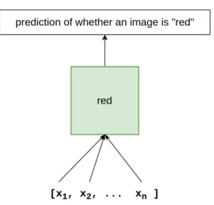
For example,to learn the grounded meaning of the word red, the low-level visual features of all images described with the word red in a corpus of image captions or descriptions are given as positive instances to a supervised learning classifier (e.g., logistic regression or multilayer perceptron), depicted in Figure 3.6. These visual features can be, for example, the RGB values of an image, or any upper layer of a CNN (i.e., transfer learning), as in [18], who we follow here. As each classifier is a binary classifier, it needs positive and negative instances; 3 negative instances are randomly sampledfrom the complementary set of images (i.e., imagesthat have

Figure3.6:StructureoftheWACmodelforthewordred.Thefeaturesofacollectionof imagesdescribedbythewordredarepassedasinputsinordertotrainabinary classifier(suchaslogisticregression).Aftertraining,theclassifierisabletoreturna

predictionofwhetheragivenimagebelongstothesemanticclass“red.”

captionsnotcontainingthewordred).Thisresultsinatrainedclassifier,towhichthe features of an image can be applied to determine how well that image is recognized as being red; inother words, a prediction of whether the image is“red.”

3.3

Embedding

WAC

Animportantbyproductof theWAC approachisthateachwordyieldsan individual classifier,andeachclassifierhasinternalstructuresthatwecanuseforotherpurposes beyond binary classification. Most classifiers (e.g., logistic regression, multi-layer perceptrons) are modeled using a set of coefficients, usually with one coefficient for eachinput feature. We can treat thesecoefficients as avector and makeuse of them in an embedded space, as is done in distributional semantic approaches.4 Such an embedding would have information about the visual grounding aspects of a word,

which is information that standard embeddings don’t have because they are only trained on text. Moreover, such an embedding can easily be combined with other existing embeddings (e.g., via concatenation).

Our prior work in Moro et al. explored the viability of using these vectors as word embeddings [33], using a simple neural network architecture of one hidden layer containing 3 nodes. Following [32], simple WAC classifiers were trained using words and images in the MSCOCO dataset and the coefficient embeddings were extracted to see if they clustered in ways that might be expected in distributional embeddings. Figure 3.7 shows the results of mapping the coefficients to 2 dimensions using t-distributed Stochastic Neighbor Embedding (TSNE) [30], and clustering the results with Density-based Spatial Clustering of Applications with Noise (dbscan) [40]. From this figure, several notable clusters include:

• yellow, red, green,blue,light, board

• area,between, of, above, edge, next to,right

• cat, dog,horse, cow,sheep,animal

These results suggest that the classifier coefficients could be used as vectors for word embeddings, as they demonstrate a similarity to embeddings, as embeddings for similar words also tend to be closer together in vector space; i.e., the cosine distance between two words represents how semantically similar they are. We further evaluate and improve on Moro et al.’s model [33], and we call our vector representation of grounded classifierswac2vec.

Figure3.7:Clustersofclassifierhiddenlayercoefficients,asshowninMoroetal.[33]. Thevocabularyisthetop100wordsfromtheMSCOCOdataset.

3.4

Training

wac2vec

Early testing using Moro et al.’s approach [33] showed mixed results on a semantic similarity task; in this thesis we use a more principled architecture, a more recent CNN for extracting image features, and reduce embeddings with PCA to eliminate noise.

We trained WAC classifiers on the Google images dataset described in Chapter 3.1. Toget imagefeatures,wepassedthe imagesthrough EfficientNet,aCNNmodel recently released by Google that achieves state-of-the-art performance on a number of datasets [42]. This resulted ina vector representationof the image that had 1000 dimensions(i.e., we use the layerdirectlybelow thepredictions layer; wedetermined this layerperformedthe bestthrough asubset ofour data onthe VisDialtask). The 1000featurevectorsforeachwordwereusedasinputfeaturestocorrespondingWAC

Figure3.8:Structureofthewac2vecredclassifier,whichhasbeentrainedon100 imagesdepictingthewordred.Theclassifiertakesinaninputof1000features,hastwo

hiddenlayersof5nodeseach,andabinarysigmoidthatoutputsthepredictionof whetheragivenimagebelongstothesemanticclass“red.”Thebottomlayerhas5005

coefficients(5000weights+5biasterms),theupperlayerhas30coefficients(25 weights+5biasterms),andthefinalbinarysigmoidhas6coefficients(5weights+1

biasterm).

classifiers,aswellasthefeaturevectorsfor3randomlysampledwords,whichserved as negative training examples.

Following[33],ourWACmodelisamulti-layerperceptron. Ourclassifiershavethe following architecture: Two hiddenlayers, eachconsisting of5 nodes; wedetermined empiricallythatthisarchitectureperformedthebestusingasubsetofourdataonpart oftheVisDialtask. Thehiddenlayersuseatanhactivationfunction,whichpreserves polarity of the coefficients (i.e., coefficient values range from -1to 1), with a binary sigmoid top layer. We trainedusing the adam solver (alpha value of 0.1 determined

through testing), an efficient optimization algorithm that converges quickly. The best parameters were found using a subset of the training data. The WAC classifiers were trained for 500 maximum epochs, with scikit-learn’s early stopping mechanism that stopped training when loss no longer improved.5

After training each classifier on its associated images, we took the coefficients from both hidden layers (testing showed that taking all the coefficients worked the best), resulting in vectors with a dimensionality of 5041 (i.e., 5 neurons in the lowest layer, each with 1000 input features; 5 neurons in the middle layer with 5 inputs each from the previous nodes; 5 inputs to the final sigmoid layer; and bias terms for each node).

Figure3.9:Graphoftheresultingdimensionalityafterreducingthewac2vecvectorsto differencevariances.

Thesevectorsaremuchlargerthanmostembeddingstendtobe,andearlytesting showed that they performed poorly on the visual dialogue task, likely due to noise

5_{We originally used Keras, a neural network library, but serialization and deserialization of trained} models was very slow, so we switched to scikit-learn, which was much faster.

in the vectors. Using PCA, we reduced the dimensionality of the vectors and opted for a balance between variance and vector size. Figure 3.9 shows a graph of the variance against dimensionality. Based on this, we chose a dimensionality of 1700, as it’s where we believed the best balance between variance and dimensionality was. However, we ran out of GPU memory when using this dimensionality on the visual dialogue task, so we decreased the dimensionality by 100 until the task was able to run successfully with the wac2vec vectors, eventually arriving at a dimensionality of 1300.

We took our resulting 1300-dimension wac2vec vectors and evaluated their perfor-mance in the NLP tasks described in Chapter 4: word similarity, named entity recognition, phrase chunking, and visual dialogue. As the visual dialogue task uses text data that is visually grounded, we used it as the standard of testing improvement in the combination of wac2vec and an embedding.

Assumptions Our wac2vec model makes two important assumptions:

1. the lexical semantics of a word is independent of all other words

2. all words are physically grounded in the physical world

For Assumption 1, this is saying that the meaning of a word has nothing to do with other words. This is clearly not the case, as we use words in a sequence, not by themselves. Assumption 2 is also not true in the real world, as there are clearly words that are abstract, like “democracy.” As discussed earlier in Section 3.1, image search results for democracy may consistently show images that contain upraised hands, but this doesn’t capture everything that democracy means. These assumptions guide how we carry out our evaluation–we concatenate the grounded wac2vec embeddings

with embeddings trained using the distributional approach, which make the opposite assumptions: that the meaning of a word depends on other words, and that all words are abstract. By combining wac2vec with distributional embeddings, we aim to mitigate these assumptions. The evaluation of our model is explained in detail in the next chapter.

CHAPTER 4

EVALUATION

To set up a pipeline for evaluating the effectiveness of wac2vec and exploring what it learns, and furthermore to establish baselines for those evaluations, we conducted a series experiments for 4 NLP tasks:

• visual dialogue

• phrase chunking

• named entity recognition

• semantic similarity

We used the visual dialogue task as our main task for testing improvements to our model. The remaining tasks were chosen because they represent tasks in order of complexity, beginning with tasks that are often used before being applied in other tasks: semantic similarity, named entity recognition, and phrase chunking. These tasks provide insight into what our model learns (or does not learn). As a task with grounded data, any improvement in performance when combining wac2vec with a traditional embedding is most likely to be shown in the visual dialogue task. In subsequent tasks, we test wac2vec’s understanding of syntax with phrase chunking and named entity recognition tasks, and finally perform a simple task, word similarity, as a test of the semantic clustering of the grounded wac2vec embeddings. In each of

these tasks, we encoded text input data with 1) standard word embedding models, including GloVe, fastText, and BERT, 2) wac2vec coefficients, and 3) embeddings concatenated with wac2vec coefficients. Following are brief descriptions of the NLP tasks that we applied wac2vec in, including an example of each task.

As mentioned above, in addition to GloVe, we also run these tasks using BERT as the distributional embedding. BERT is a recent neural network architecture that has been setting the state of the art for many NLP tasks. We put a single word at a time through BERT in order to create BERT embeddings; in tasks like visual dialogue that use a full sentence, we would want to pass the entire sentence into BERT in order to make use of context (i.e. “stood on the river’s bank” vs. “she robbed a bank”). However, due to limitations of our hardware, we were unable to utilize BERT in this way for the visual dialogue task, though we able to do so in the named entity recognition and noun phrase chunking tasks.

4.1

Visual Dialogue

This task, unlike the others, incorporates a visual element in addition to text data. In visual dialogue, the goal is to answer questions about an image, particularly in the context of previous asked and answered questions. In other words, this task incorporates visual as well as lexical context.

Question: How many people are there? [Answer: Two]

Question: Are they standing? [Answer: No, they are sitting]

4.1.1 Task & Procedure

We follow Massiceti et al. for this, using the model created and provided by [31], which uses the MSCOCO dataset [25], and we used both GloVe and BERT embed-dings.1 _{Aside from specifying the final dimensionality of the provided embeddings} (i.e. wac2vec concatenated with BERT) and setting the batch size to 16 (in order to avoid running out of memory), we leave all settings as were defined in Massiceti et al. In their approach, prior dialogue context and features of the image being discussed are not used; the authors claim that the task can be approached with just the question-answer pair, and as the wac2vec vectors are applied directly to the words in the question-answer pairs, we don’t need images to evaluate the effectiveness of our model in this task. Their model learns joint embeddings between questions and answers by calculating projection matrices (one for questions and one for answers), with the goal of maximizing the correlation between projections of each matrix. At test time, candidate answers are ranked by the cosine distance between the joint 1_{The code we used for this task can be found at https://github.com/danielamassiceti/} CCA-visualdialogue

Model MR R@1 R@5 R@10 MRR Baseline (fastText) 16.2052 16.8566 44.9837 58.0817 0.3043 GloVe 18.6441 13.9362 38.1933 51.7285 0.2623 BERT 14.4935 18.4362 47.0531 60.9851 0.3530 wac2vec 15.3334 19.1011 46.7808 60.9582 0.3249 wac2vec + GloVe 14.9333 20.3313 49.2361 62.6997 0.3409 wac2vec + BERT 14.9250 20.7824 49.2855 62.3896 0.3441 Baseline (fastText) 17.0314 16.0320 41.1822 55.1938 0.2860 GloVe 19.9415 13.9244 35.8527 49.6657 0.2540 BERT 15.5700 17.6744 43.9874 58.2219 0.3052 wac2vec 15.9998 17.3934 42.9264 58.3333 0.3017 wac2vec + GloVe 15.4788 18.2897 44.7384 59.6415 0.3131 wac2vec + BERT 15.6268 18.7888 44.9128 59.1667 0.3166

embeddings of the question and each candidate answer, drawing upon the semantic similarity of questions and potential answers,rather than image data. They encode questions and answers using fastText embeddings; we replace these with our own (wac2vec,GloVe, BERT, wac2vec +GloVe, and wac2vec +BERT).

We tested on both versions of the dataset that they used (i.e., version 0.9 and 1.0), providedby [10].

4.1.2 Metrics

In this task, the goal is to rank 100 possible answers to a question about an image, with only one answer being the correct one. This task uses a number of metrics: 1) mean rank (i.e., the average ranked position of the correct answer); 2) recall r@k Table 4.1: Results from the visual dialogue task. The top half of the results are for the v0.9 dataset, and the bottom half are for the v1.0 dataset. From left to right, metrics are: mean rank; recall at 1, 5, and 10; and mean reciprocal rank. Best results are bolded. For best results that combine wac2vec and an embedding, we calculated the statistical significance using a paired t-test, with an alpha of 0.05. Our null hypothesis was that wac2vec does not improve the performance of the

distributional embedding. With p-values of <0.01 for each result we tested, we found that these best-performing results were statistically significant.

considering up to positions @5, @10, and @15; and 3) mean reciprocal rank mrr, where ranki is the position of the correct answer for the i-th question in the Q

dataset. r@k= T P T P +F N (4.1) mrr= 1 |Q| |Q| X i=1 1 ranki (4.2) 4.1.3 Results

Table 4.1 shows the results from the visual dialogue task, on both version 0.9 and 1.0 of the visual dialogue dataset. As can be seen, combining wac2vec with GloVe and BERT embeddings improves performance on nearly all metrics for both datasets. Furthermore, wac2vec on its own performs better than both GloVe and the fastText baseline used by Massiceti et al., on both versions of the VisDial dataset.

These results suggest that wac2vec is able to contribute additional semantic in-formation that BERT, which has demonstrated state-of-the-art performance on a number of NLP tasks, as well as GloVe, do not have on their own. This is partic-ularly interesting for this task because neither BERT, GloVe, nor wac2vec actually visually inspect the images directly–rather, they are just using the question-answer pairs, but wac2vec adds visually important semantic information. As the VisDial question-answer dataset is strongly grounded (i.e., many words about things that are physically represented in a photograph), it makes sense that wac2vec, a grounded model, would do well here when used as an embedding for these words. This is supported by the individual results for wac2vec, which performs better than the

fastText and GloVe embeddings across all metrics.

The resulting performance of combining wac2vec with traditional embeddings in this task suggests that wac2vec provides semantic information that embeddings trained on text lack. However, what else does wac2vec learn? We explore this in the following experiments.

4.2

Phrase Chunking

The phrase chunking task involves identifying and extracting phrase chunks from text, and requires an understanding of syntax. The following example depicts extraction of noun phrase chunks from a sentence.

[The little yellow dog] barked at [the cat].

4.2.1 Task & Procedure

Following [3], this task involved locating and classifying phrase chunks in the CoNLL-2000 [37] corpus, as described in Section 3.1.

In addition to GloVe and BERT, we used Flair embeddings from the Flair library,2 to test against the baseline in [3]. The Flair library also provides BERT embeddings that can be used in this task, which operate over the entire sentence rather than each word individually. Following the work in [3], this task uses an LSTM that is trained for a max of 150 epochs.3 _{Sentences are encoded using the embeddings, and} the LSTM predicts the phrase chunk tag for each word in the sentence.

2_{https://github.com/zalandoresearch/flair}

3_{The code we used for the phrase chunking task is available at https:} //github.com/flairNLP/flair/blob/master/resources/docs/EXPERIMENTS.md#

conll-2000-noun-phrase-chunking-english. While this page calls it noun phrase chunking, it is actually a general chunking task, and predicts multiple types of phrase chunks (for example, verb phrase and adjective phrase).

4.2.2 Metrics

Following [3], results are evaluated using the F1 score, the harmonic mean of precision pand recallr, over correctly identifying the phrase tags of the words in each sentence. In addition, we also report the accuracy a of correctly identifying the phrase tag of each word. T P, F P, T N, and F N are the number of true positives, false positives, true negatives, and false negatives found during evaluation of predicted phrase tags, respectively. p= T P T P +F P (4.3) r = T P T P +F N (4.4) F1 = 2∗ p∗r p+r (4.5) a= T P +T N T P +F P +T N +F N (4.6) 4.2.3 Results

In this task, BERT from the Flair library performed highest out of all the single embeddings; wac2vec performed the lowest. As shown in Table 4.2, combining wac2vec with the distributional word embeddings yielded no benefit, save for in the combination of BERT and wac2vec, which provided a small improvement on F1 score and accuracy over BERT alone.4 _{Noun phrases are a type of phrase chunk found in the} 4_{We do not perform statistical significance tests on the results of this or subsequent experiments,} as any improvements when adding wac2vec to traditional embeddings are very small, and we derive

Model F1 score Accuracy Flair (baseline) 0.9640 0.9305 wac2vec 0.8550 0.7467 GloVe 0.9382 0.8836 BERT 0.8780 0.7825 BERT* 0.9659 0.9342 wac2vec + Flair 0.9524 0.9092 wac2vec + GloVe 0.9229 0.8568 wac2vec + BERT 0.8550 0.7467 wac2vec + BERT* 0.9667 0.9356

dataset of this task, and nouns tend to be concrete, which may explain why results were better here. However, as the improvement was small, and as other wac2vec combinations showed no improvement, it’s possible this result was due to chance. Our results forthis task generallysuggest that wac2vecdoes not learn syntax,which is tobeexpected, aswac2vec makes an assumptionof lexical wordindependence.

4.3

Named

Entity

Recognition

Named entity recognition (NER) involves locating and classifying named entities within text. Like phrase chunking, this task is also mostly a test of syntax. Named entitiescan includepeople,organizations, locations, expressionsof time, and others.

[Janet]Person started working at[Twitter]Organization in[2010]Time.

no final conclusion from them.

Table 4.2: Results from the chunking task. The two metrics here are F1 score and accuracy. Starred BERT indicates BERT provided by the Flair library. Best results are bolded.

4.3.1 Task & Procedure

In this task, named entities were identified and extracted from the CoNLL-2003 [38] corpus, described in Section 3.1. As in the phrase chunking task, we follow [3] and tested Flair embeddings in addition to GloVe and BERT embeddings, as well as BERT from the Flair library. Also like the phrase chunking task, the NER task uses an LSTM that is trained for a max of 150 epochs; the input is encoded sentences (using our provided embeddings), and the LSTM predicts the named entity tag of each word in the sentence.5

4.3.2 Metrics

Like the phrase chunking task, following [3], results are evaluated using the F1 score and accuracy over correctly identifying a word’s named entity tag. Shown in Table 4.2 are the results for this task.

4.3.3 Results

In this task, Flair performed better than wac2vec, GloVe, both versions of BERT, and all of the wac2vec + embedding combinations. The dataset for this task, as to be expected, has a large number of named entities such as names and numbers, which are not as well represented by images (i.e., they are abstract concepts) and likely resulted in less effective WAC classifiers and therefore weaker wac2vec vectors. Also interesting to note is that while wac2vec combinations do not provide the highest results, wac2vec does improve the results for single-word BERT embeddings; however, these results are superceded by those of BERT from the Flair library, in which BERT 5_{For the NER task, we used the code available athttps://github.com/flairNLP/flair/blob/} master/resources/docs/EXPERIMENTS.md#conll-03-named-entity-recognition-english.

Model F1 score Accuracy Flair (baseline) 0.9235 0.8578 wac2vec 0.7381 0.5849 GloVe 0.8882 0.7988 BERT 0.6304 0.4603 BERT* 0.9131 0.8401 wac2vec + Flair 0.9017 0.8209 wac2vec + GloVe 0.8508 0.7403 wac2vec + BERT 0.7719 0.6284 wac2vec + BERT* 0.9113 0.8371

is properly used at the sentence level. Like in the phrase chunking task, wac2vec by itselfperforms poorly in this task.

4.4

Word

Similarity

Wordsimilaritygivesascoreofhowaliketwowordsaretoeachotherinavectorspace. This is useful because standard embeddings and our wac2vec model are represented as vectors, with the assumption that two vectors that are close in vector space are semantically similar. This is the simplest of all our tasks, as it simply involves calculating how close together two embeddings for a word pair are in vector space, using cosine similarity(explainedbelow).

coast -shore [very similar] tree - car [not similar]

Table 4.3: Results from the named entity recognition task. The two metrics here are F1 score and accuracy. Starred BERT indicates BERT provided by the Flair library. Best results are bolded.

4.4.1 Task & Procedure

The task involved predicting the semantic similarity of words pairs in two datasets, WordSim-353 and SimLex-999 (see Section 3.1).6

We tested a number of embedding combinations, using both GloVe and BERT, to compare the relative benefits of applying wac2vec to different models. See Table 4.4 for a list of all embeddings tested. The cosine similarity between the embeddings of two words in a pair is calculated with:

vec1 ·vec2 ||vec1||||vec2||

(4.7)

wherevec1is the embedding of the first word in the pair, andvec2is the embedding of the second word in the pair.

4.4.2 Metrics

Following prior work [36], our metric for this task was the Spearman correlation, as a way to aggregate the cosine similarities between words in the datasets. This task uses the spearmanr method provided by the SciPy Python library, and calculates the Spearman correlationrs over ranked word similaritiesrx provided by a particular

embedding and the ranked known similarities ry provided by the dataset. In the

following equation, cov(rx, ry) is the covariance of rx and ry, andσrx and σry are the

standard deviations of rx and ry, respectively.

rs =

cov(rx, ry)

σrxσry

(4.8)

6_{We used code from this project to calculate similarity between word pairs: https://github.} com/recski/wordsim

Model Spearman wac2vec 0.0198 GloVe 0.3392 BERT 0.1582 wac2vec + GloVe 0.0585 wac2vec + BERT 0.0618 wac2vec 0.1565 GloVe 0.6312 BERT 0.3750 wac2vec + GloVe 0.2503 wac2vec + BERT 0.2990 4.4.3 Results

Table 4.4 shows the results for this task. As can be seen, for both the SimLex-999 dataset and the WordSim-999 dataset, adding wac2vec toeither of the two distribu-tional embeddingsdid nothing toimprove results.

Somethinginterestingintheseresultsisthat BERTisfaroutperformedbyGloVe, despite it setting the state of the art on many other NLP tasks. We speculate this is because of the nature of BERT–a task such as this is situated purely onthe word level,ratherthanthesentencelevel,whereBERTisabletoworkbest. Unexpectedly, wac2vec does not perform well in this task. It would seem that it does not capture representations invector space as well as we would havethought.

4.5

Discussion

of

Results

In this chapter, we evaluated wac2vec, and the combination of wac2vec and a tra-ditional distributional embedding, on several NLP tasks: visual dialogue, phrase

Table 4.4: Results from the word similarity task. The top half of the results correspond to the SimLex-999 dataset, and the bottom half shows results on the WordSim-353 dataset. The metric used in this task is the Spearman correlation. Best results are bolded.

chunking, named entity recognition, and word similarity.

Wac2vec, an embedding model that is applied directly to words, performs well on its own in visual dialogue, a task that contains a high number of concrete, visually-grounded words. Furthermore, the performance of traditional word embeddings was improved when combined with wac2vec embeddings. We believe this demonstrates that wac2vec, which is trained on visual data, enriches traditional embeddings, which are trained on text data.

While wac2vec does perform well and improve performance for distributional embeddings on our visually grounded task, it does not do so for the named entity recognition and phrase chunking tasks, which are generally tests of syntax (named entities are usually noun phrases that do not necessarily denote concrete things). The fact that wac2vec neither performs well by itself nor tends to improve performance when concatenated to traditional embeddings suggests that wac2vec does not learn syntax. These results are understandable, as wac2vec makes an assumption of lexical independence–the classifier for each word is trained independently of all other words. Another reason for the poor results of these two tasks could be that the datasets they use contain much less grounded language than the dataset used in the visual dialogue task.

One thing to consider is whether the larger embedding size of wac2vec contributes to higher performance, rather than the presence of important visual information in our vectors. After all, in the visual dialogue task, wac2vec, with its very large vector of 1300, consistently performed better than both fastText and GloVe on all metrics. However, it was almost always outperformed by BERT, a smaller vector at size 768, and in the other three tasks, wac2vec tended to perform the lowest, with no improvement when combining with traditional embeddings. Because of this,

we believe that wac2vec’s performance in the visual dialogue task, both alone and when concatenated to another embedding, is not due to its higher dimensionality (in comparison to the other embeddings).

CHAPTER 5

CONCLUSIONS

5.1

What have we done so far?

In this thesis, we have evaluated wac2vec, a model that draws upon grounded se-mantics by training individual word classifiers on a collection of images downloaded from image search engines, using a vocabulary derived from the Age of Acquisition dataset and the datasets used in evaluation of our model. We extracted the coefficients from these classifiers to form grounded word embeddings, and combined them with traditional word embeddings that model distributional semantic meaning. Finally, we conducted empirical analysis upon our model to gain insight into what it learns and whether it enriches text-only embeddings, using four NLP tasks: visual dialogue, phrase chunking, named entity recognition, and word similarity.

For most of our tasks, concatenating wac2vec with distributional embeddings tended to not improve performance. This was not unexpected: I conjecture that this is likely because the phrase chunking and named entity recognition tasks are mostly tests of syntax, whereas our model makes an assumption of the independence of words; it makes sense that it would not handle syntactic tasks well.

We did, however, observe improvements in the visual dialogue task when com-bining wac2vec with both GloVe and BERT embeddings, in comparison to these embeddings alone. The visual dialogue dataset is a visually-grounded task, and

contains concrete language referring to and describing a series of images. The fact that performance is improved on this task when combining wac2vec and traditional embeddings suggests that wac2vec successfully provides grounded semantic informa-tion not captured by these embeddings.

In conclusion, we find that combining wac2vec, which is grounded, with a distribu-tional embedding adds important semantic information, as performance is improved when using both together in a visual task (as opposed to either of the two alone). This has implications for any task that might use concrete words (e.g., visual dialogue, visual question answering, reference resolution, and interaction with robots). As ex-pected, it does not help performance in more syntactically-oriented tasks, suggesting WAC doesn’t learn anything about syntax; the wac2vec vectors should always be used in conjunction with proper distributional embeddings such as GloVe or BERT.

5.2

Future Directions

In future work, we will perform weighting of words according to concreteness. Words that are more abstract will be weighted more towards embeddings, and those that are more concrete will be weighted more towards wac2vec. We also want to explore how wac2vec works with the full power of a BERT-like transformer model; in this thesis, we only extracted word embeddings for BERT by passing a single word at a time through the BERT model, instead of passing an entire sentence, due to the limitations of our hardware. This was a valid approach for the word similarity task (as there are no sentences, only individual words), but the visual dialogue task, which uses questions and answers, would benefit from passing the entire sentence into BERT.