TI 2011-007/4
Tinbergen Institute Discussion Paper
Nonlinear Forecasting with Many
Predictors using Kernel Ridge
Regression
Peter Exterkate*
Patrick J.F. Groenen
Christiaan Heij
Dick van Dijk*
Econometric Institute, Erasmus School of Economics, Erasmus University Rotterdam. * Tinbergen Institute
Tinbergen Institute is the graduate school and research institute in economics of Erasmus University Rotterdam, the University of Amsterdam and VU University Amsterdam. More TI discussion papers can be downloaded at http://www.tinbergen.nl
Tinbergen Institute has two locations: Tinbergen Institute Amsterdam Gustav Mahlerplein 117 1082 MS Amsterdam The Netherlands Tel.: +31(0)20 525 1600 Tinbergen Institute Rotterdam Burg. Oudlaan 50
3062 PA Rotterdam The Netherlands Tel.: +31(0)10 408 8900 Fax: +31(0)10 408 9031
Duisenberg school of finance is a collaboration of the Dutch financial sector and universities, with the ambition to support innovative research and offer top quality academic education in core areas of finance.
DSF research papers can be downloaded at: http://www.dsf.nl/
Duisenberg school of finance Gustav Mahlerplein 117 1082 MS Amsterdam The Netherlands Tel.: +31(0)20 525 8579
Nonlinear Forecasting With Many Predictors
Using Kernel Ridge Regression
∗Peter Exterkate† Patrick J.F. Groenen Christiaan Heij Dick van Dijk
Econometric Institute, Erasmus University Rotterdam
January 4, 2011
Abstract
This paper puts forward kernel ridge regression as an approach for forecasting with many predic-tors that are related nonlinearly to the target variable. In kernel ridge regression, the observed predictor variables are mapped nonlinearly into a high-dimensional space, where estimation of the predictive regres-sion model is based on a shrinkage estimator to avoid overfitting. We extend the kernel ridge regresregres-sion methodology to enable its use for economic time-series forecasting, by including lags of the dependent variable or other individual variables as predictors, as is typically desired in macroeconomic and finan-cial applications. Monte Carlo simulations as well as an empirical application to various key measures of real economic activity confirm that kernel ridge regression can produce more accurate forecasts than traditional linear methods for dealing with many predictors based on principal component regression.
Keywords:High dimensionality, nonlinear forecasting, ridge regression, kernel methods.
JEL Classification:C53, C63, E27.
∗
We thank conference participants at the International Conferences on Computational and Financial Econometrics in 2009 and 2010, at Eurostat in Luxembourg, and at Cass Business School in London, United Kingdom, for useful comments and suggestions.
†
Corresponding author. Address: Econometric Institute, Erasmus University Rotterdam, P.O. Box 1738, 3000 DR Rotterdam, The Netherlands; email: [email protected]; phone: +31-10-4081264; fax: +31-10-4089162.
1
INTRODUCTION
In current practice, forecasters in macroeconomics and finance face a trade-off between model complexity and forecast accuracy. Due to the uncertainty associated with model choice and estimation, a highly com-plex predictive regression model based on many variables or intricate nonlinear structures is often found to produce less accurate forecasts than a simpler model that ignores major parts of the information that is at the researcher’s disposal. Various methods for working with many predictors while circumventing thiscurse of dimensionalityin a linear framework have been applied in the recent forecasting literature, as surveyed by Stock and Watson (2006). Most prominently, Stock and Watson (2002) advocate summarizing large panels of predictor variables into a small number of principal components, which are then used for forecasting purposes in a dynamic factor model. Alternative approaches include combining forecasts based on multiple models, each of which includes only a small number of variables (Faust and Wright, 2009; Wright, 2009; Aiolfi and Favero, 2005; Huang and Lee, 2010; Rapach et al., 2010), partial least squares (Groen and Kapetanios, 2008), and Bayesian regression (De Mol et al., 2008). Stock and Watson (2009) find that for forecasting macroeco-nomic time series, the dynamic factor model is preferable to these alternatives; see also Ludvigson and Ng (2007), Ludvigson and Ng (2009) and C¸ akmaklı and van Dijk (2010) for successful applications in finance.
The possibility of nonlinear relations among macroeconomic and financial time series has also received ample attention during the last two decades. Among the most popular nonlinear forecast methods are regime-switching models and neural networks, see the surveys by Ter¨asvirta (2006) and White (2006), respectively. Typically, these approaches are only suitable for small numbers of predictors, and even then their ability to improve upon the predictive accuracy of conventional linear forecasting techniques seems limited, see Stock and Watson (1999); Medeiros et al. (2006); Ter¨asvirta et al. (2005).
In this paper, we introduce a forecasting technique that can deal with high-dimensionality and nonlinearity simultaneously. The central idea of this approach, known askernel ridge regression, is to map the set of pre-dictors into a high-dimensional (or even infinite-dimensional) space in a nonlinear way. A forecast equation is estimated in this high-dimensional space, using a penalty (or shrinkage, or ridge) term to avoid overfitting. In this manner, kernel ridge regression averts the curse of dimensionality, which plagues alternative nonparamet-ric approaches to allow for flexible types of nonlinearity (Pagan and Ullah, 1999). Computational tractability
is achieved by choosing the kernel in a convenient way, so that calculations in the high-dimensional space actually are prevented. This approach avoids computational difficulties also encountered in standard ridge regression when the number of predictor variables is large relative to the number of time series observations. Taking all these elements together, kernel ridge regression provides an attractive framework for estimating nonlinear relations in a data-rich environment.
The kernel methodology has been developed in the machine learning community, an area in which re-searchers often work with large data sets. A typical application is optical recognition of pixel-for-pixel scans of handwritten characters. Sch¨olkopf et al. (1998) document outstanding performance of kernel methods for this classification task. Kernel ridge regression has been found to work well also in many other applications. Time-series applications are scarce and seem to be limited to deterministic (that is, non-stochastic) time se-ries (M¨uller et al., 1997). Kernel ridge regression has, to our knowledge, not yet been applied in the context of macroeconomic or financial time-series forecasting. In this paper, we extend the kernel methodology to facilitate the estimation of models that include lags of the dependent variable or other individual variables as predictors, as is typically desired in such applications. Using Monte Carlo simulations, we demonstrate that kernel ridge regression delivers more accurate forecasts than conventional methods based on principal com-ponents in the presence of many predictors that are related nonlinearly with the target variable. These conven-tional methods include the extensions of the principal component regression methodology to accommodate nonlinearity as put forward by Bai and Ng (2008). The potential practical usefulness of kernel methods is confirmed in an empirical application to forecasting several key measures of U.S. macroeconomic activity over the period 1970-2009. We find that, when traditional methods perform poorly, kernel ridge regres-sion yields substantial improvements. This result holds for Industrial Production and for Personal Income. Further, when traditional forecasts are of good quality, as is the case for the Sales and Employment series, kernel-based forecasts remain competitive. We also find that kernel ridge regression is much less affected by the recent financial and economic crisis in 2008-9 than the traditional methods are.
The remainder of this paper is organized as follows. Section 2 describes the kernel methodology. The Monte Carlo simulation is presented in Section 3, and Section 4 discusses the empirical application. Conclu-sions are provided in Section 5.
2
METHODOLOGY
The technique of kernel ridge regression is based on ordinary least squares regression and ridge regression. Therefore, we begin this section with a brief review of these methods, highlighting their drawbacks in dealing with nonlinearity and high-dimensionality. Next, we show how kernel ridge regression overcomes these drawbacks by means of the so-calledkernel trick. We also present the properties of some kernel functions that are popular because of their computational efficiency. As will become clear below, kernel ridge regression involves tuning parameters. We close this section with a description of a cross-validation procedure for selecting values for these parameters.
2.1 Preliminaries
Consider the following general setup for forecasting. At the end of periodT we wish to forecast the value of a target variableyat a specific future date, denotedy∗, given anN ×1vector of predictorsx∗. Historical observations fort = 1, . . . , T are available on all variables, collected in theT ×1vectoryand theT ×N
matrixX. If we assume a linear prediction functiony∗ˆ = x0∗βˆand obtain βˆ by minimizing the ordinary least squares criterion||y−Xβ||2, the solution isβˆ= (X0X)−1X0y, provided thatX has rankN, and the corresponding forecast isy∗ˆ =x0∗(X0X)−1X0y.
The ordinary least squares procedure presupposes thatN ≤ T, and in practice,N T is required to prevent overfitting problems. That is, ifN is not small compared toT, we may obtain a good in-sample fit (indeed, ifN =T, the in-sample fit will be perfect), but the out-of-sample predictiony∗ˆ is generally found to be of poor quality. A possible solution to this problem is shrinkage estimation or ridge regression, which aims to balance the goodness-of-fit and the magnitude of the coefficient vectorβ. The ridge criterion is given by||y−Xβ||2 +λ||β||2, where the penalty parameter λ > 0 is to be specified by the user. Minimizing this criterion is most easily done by performing ordinary least squares on the (T +N) ×1 vector u =
y0,00N×10
and the(T+N)×N matrix V = X0,√λ IN×N
0
, as we may then write ||y−Xβ||2 +
λ||β||2 = ||u−V β||2. This criterion is minimized by βˆ = (V0V)−1V0u, or, in terms of the original variables,βˆ = (X0X+λI)−1X0y. The resulting forecasty∗ˆ = x0∗(X0X+λI)
−1
X0y can be computed also if the number of predictorsN is larger than the number of observationsT. Nevertheless, if the number
of regressors becomes very large, the calculation of the ridge forecast may present computational difficulties, as it involves inverting a possibly ill-conditionedN ×N matrix. In practice, this hampers the use of ridge regression whenN T, unless the shrinkage parameterλis taken to be very large.
2.2 Kernel Ridge Regression and the Kernel Trick
Kernel ridge regression extends the general setup considered above to allow for nonlinear prediction functions
ˆ
y∗ = f(x∗). At the same time, it provides a way to avoid the computational complications involved in producing the ridge forecast when the number of predictors becomes very large. As will become clear below, this is particularly relevant in the context of nonlinear forecasting. From now on, letN denote the number of observed predictor variablesx, and let ϕ : RN → RM be a (possibly nonlinear) mapping resulting in M transformed predictor variables. We assume that the prediction function is linear in z = ϕ(x), say
ˆ
y∗ = z∗0γˆ, where z∗ = ϕ(x∗). Collecting the transformed predictor variables in the T ×M matrix Z
with rowszt0 =ϕ(xt)0, we may apply ridge regression to obtainγˆ = (Z0Z+λI)−1Z0y, and hence,y∗ˆ =
z∗0 (Z0Z+λI)−1Z0y.
In macroeconomic and financial applications we often work with high-dimensional data, sometimes with the number of observed predictorsNexceeding the number of time series observationsT. Moreover, to allow for flexible forms of nonlinearity in the forecast equation, we needM N. For example, if we approximate the unknown forecast functionf by adth order Taylor expansion, the mappingϕeffectively transforms the
N ×1 vectorx into the M ×1 vector z containing powers and cross-products of its elements, withM
proportional toNd. Thus,M may become extremely large for realistic values ofNandd. As the matrixZ0Z
has dimensionsM×M, this can cause computational difficulties in producing the nonlinear ridge forecast. An efficient method to solve this curse of dimensionality problem is provided by the so-called kernel trick. Essentially this method is based on the idea that if the number of regressorsMis much larger than the number of observations T, working with T-dimensional instead of M-dimensional quantities can lead to notable computational savings. To appreciate the dimension reductions involved, we consider the macroeconomic application that will be discussed in Section 4. In this application, we estimate models with N = 132
all observed predictors, their squares, and the cross-products of all pairs of predictors, leading to a total of
M = (N + 1) (N+ 2)/2 = 8911 transformed predictor variables. The results that we describe in the remainder of this section allow working with a120×120matrix instead of the8911×8911matrixZ0Z.
This dimension reduction can be achieved by some algebraic manipulations of the expression of the non-linear ridge forecast equationy∗ˆ =z0∗ˆγ. First, we rewrite the ridge regression estimatorˆγ= (Z0Z+λI)−1Z0y
asZ0Zγˆ+λγˆ=Z0y, or ˆ γ = 1 λ Z 0y−Z0Zγˆ = 1 λZ 0(y−Zˆγ).
If we pre-multiplyZ0Zˆγ+λγˆ=Z0yby the matrixZ, this givesZZ0Zˆγ+λZγˆ=ZZ0y, or
Zˆγ= ZZ0+λI−1
ZZ0y.
Combining these two results, we find
ˆ y∗ = z∗0γˆ = 1 λz 0 ∗Z0(y−Zγˆ) = 1 λz 0 ∗Z0 y− ZZ0+λI−1 ZZ0y = 1 λz 0 ∗Z0 ZZ0+λI −1 ZZ0+λI−ZZ0 y = z∗0Z0 ZZ0+λI−1 y.
If we define theT×T matrixK =ZZ0and theT ×1vectork∗=Zz∗, this result can be written as
ˆ
y∗=k∗0 (K+λI)−1y. (1)
The inverse matrix in Equation (1) has dimensions T ×T, so that no M-dimensional computations are required to determine the forecasty∗ˆ , onceKandk∗are known. To achieve computational savings over the straightforward application of ridge regression, it is crucial thatK andk∗ can be computed in a relatively simple way. The(s, t)th element ofK = ZZ0 equalszs0zt = ϕ(xs)0ϕ(xt), and similarly, the tth element
ofk∗ equals ϕ(xt)0ϕ(x∗). This implies that the computational efficiency increases greatly if we choose
a mappingϕfor which the inner productκ(a, b) = ϕ(a)0ϕ(b) can be computed quickly, that is, without computingϕ(a) and ϕ(b) explicitly. In this context, κ is called the kernel function and K is thekernel matrix. This procedure for implicitly finding the optimal parameter vector γˆ in the “high” dimension M
while working exclusively in the “low” dimensionT is known as thekernel trick and is due to Boser et al. (1992).
As the above discussion shows, kernel ridge regression is no different from ordinary ridge regression on transformations of the regressors, except for an algebraic trick to improve computational efficiency. The key to a successful application of this kernel trick is choosing a mappingϕthat leads to an easy-to-compute kernel functionκ. Various such mappings are known, and a recent overview is given in Smola and Sch¨olkopf (2004). The next section presents the most commonly used instances of these mappings.
We close this section by noting that in a time series context, we often prefer to include some specific predictors in the forecast equation separately from the nonlinear mappingϕ. In macroeconomic applications, these predictors may include lags of the dependent variable to account for serial correlation. In financial ap-plications such as predicting stock returns, these predictors may include valuation ratios such as the dividend yield or interest rate related variables; see Ludvigson and Ng (2007), C¸ akmaklı and van Dijk (2010), for ex-ample. In such cases we consider the generalized forecast equationy∗ˆ =w∗0βˆ+z∗0γˆ, where theP×1vector
w∗contains the variables to be treated linearly. We collect the historical observations on these variables in the
T×P matrixW. We show in Appendix A.1 that the derivations that lead to (1) can be extended to include such linear terms, resulting in the “extended” kernel ridge regression forecast equation
ˆ y∗ = k∗ w∗ 0 K+λI W W0 0 −1 y 0 . (2)
This is the forecast equation that will be used in the empirical application in Section 4.
2.3 Some Common Kernel Functions
A first and obvious example is the identity mappingϕ(a) = a, for whichκ(a, b) = a0b. With this choice ofκ, the kernel forecast y∗ˆ = k0∗(K+λI)−1y = x0∗X0(XX0+λI)−1y equals the linear ridge forecast
ˆ
y∗ = x0∗(X0X+λI)−1X0y, as can be seen by takingZ = X andz∗ = x∗ in the derivations preceding Equation (1).
squares and cross products of these variables. Some experimentation reveals thatκ(a, b)takes a particularly simple form if we multiply some elements ofϕ(a)by the constant√2. That is, if we choose the mapping
ϕ(a) =1,√2a1, √ 2a2, . . . , √ 2aN, a21, a22, . . . , a2N, √ 2a1a2, √ 2a1a3, . . . , √ 2aN−1aN 0 ,
the corresponding kernel function is
κ(a, b) =ϕ(a)0ϕ(b)
= 1 + 2 (a1b1+a2b2+. . .+aNbN) +a12b21+a22b22+. . .+a2Nb2N
+ 2 (a1a2b1b2+a1a3b1b3+. . .+aN−1aNbN−1bN)
= 1 + 2 (a1b1+a2b2+. . .+aNbN) + (a1b1+a2b2+. . .+aNbN)2
= 1 + 2a0b+ a0b2 = 1 +a0b2.
With this specification of the kernel function, the computation of each of theT(T+ 1)/2distinct elements of the kernel matrixKrequires2 (N+ 1)additions and multiplications. In the absence of the indicated scaling, the vector of constant, first-order, and second-order terms containsM = (N+ 1) (N + 2)/2elements. The computation of each element of the kernel matrix would then require2M = (N+ 1) (N + 2)additions and multiplications. Thus, the proposed scaling reduces the amount of computations by a factor of1 +N/2.
As noted by Poggio (1975), this result can be generalized to the kernel function
κ(a, b) = 1 +a0bd for any integerd≥1, (3) corresponding to a mapping for whichϕ(a) consists of all polynomials in the elements ofaof degree at mostd. Observe that this class of so-called polynomial kernel functions encompasses not only the quadratic mapping, ford= 2, but also the identity mapping (and hence, standard linear ridge regression), ford= 1.
Because smart choices of ϕenable us to avoid M-dimensional computations, the kernel methodology even allows lettingM → ∞. A common way to do this, dating back to Broomhead and Lowe (1988), is by
using the Gaussian kernel function κ(a, b) = exp −1 2||a−b|| 2 . (4)
We show in Appendix A.2 that the corresponding mapping ϕ(a) contains as elements, for all degrees
d1, d2, . . . , dN ≥0, the “dampened” polynomials
e−a0a/2 N Y n=1 adn n √ dn! .
In this paper, we consider the polynomial kernels (3) of degreesd = 1and2, as well as the Gaussian kernel (4). To control for the relative importance of the terms inϕ(x), we replace each observation x by
(1/σ)x before computingκ, for some positive scaling factorσ. Such scaling affects the weight placed on different polynomial degrees, as it amounts to dividing linear terms inϕ(x)byσ, second-order terms byσ2, and so forth. Although we are performing linear regression onϕ(x), such scaling is not without effect, as its regression coefficients in the forecast equationy∗ˆ = w∗0βˆ+ϕ(x∗)
0
ˆ
γ are all penalized equally by the ridge term in the criterion function||y−W β−Zγ||2+λ||γ||2.
2.4 Selection of Tuning Parameters
Our implementation of kernel ridge regression contains two tuning parameters, namely, the shrinkage param-eterλand the scaling parameterσ. Additionally, our empirical application in Section 4 to several macroeco-nomic time series involves the selection of lag lengths, which can also be seen as tuning parameters from a model selection perspective. This section addresses the question of how to set the values for these parameters. We determine the values of the tuning parameters by means of leave-one-out cross-validation, as this is a natural criterion for the purpose of out-of-sample forecasting. For given values of the tuning parameters, we estimate the model on the sample of sizeT −1that remains when the observation for periodtis removed. We then use this model to “forecast” the value ofytthat was left out. This is repeatedT times, leaving out
each observation fort= 1, . . . , T once. Performing this cross-validation exercise for each of the candidate values of the tuning parameters, we select those values that lead to the smallest mean squared prediction error
over theseT forecasts. These values are then used to estimate the model on the full sample1,2, . . . , T, from which we produce out-of-sample forecasts.
In the form stated above, this cross-validation procedure is computationally very expensive, as it requires estimating the model onT different samples for each possible setting of the tuning parameters. Cawley and Talbot (2008) propose a method that yields all leave-one-out prediction errors as a by-product of estimating (1) only once, that is, on the full sample. We derive a similar result, extended to allow for the additional linear terms in (2), in Appendix A.3.
In the simulation examples and in the empirical study below, we use this method to select both the lag lengths and the ridge parameterλfrom a grid. Because we will use rolling-window estimation, these parameter values are reselected for each forecast. As it is difficult to find intuitively reasonable values for the shrinkage parameter, we employ a fairly wide grid, containing 45 candidate values:
log10(λ) ∈ {−8,−5,−4.0,−3.8,−3.6, . . . ,3.6,3.8,4.0,5,8}.
The same cross-validation procedure could also be used to select the scaling parameterσ. Preliminary simulation evidence shows that it is difficult to identifyλandσsimultaneously from data, as a wide range of
(λ, σ)combinations is found to lead to very similar forecasts. Relatively little out-of-sample forecast quality is sacrificed if the scaling parameterσis fixed a priori. Based on these exploratory results, we rescale the data to have mean zero and variance one and then we use, as a practical rule of thumb,σ= 2dfor the polynomial kernel of degreedandσ= 10for the Gaussian kernel.
As a technical note, serial correlation in time-series data leads to dependence between the observations in the estimation sample and the observation that was left out. This dependence implies that the standard leave-one-out cross-validation procedure may not be fully adequate; see Racine (2000) for an extensive discussion and a modification to overcome these problems. Although the method outlined in Appendix A.3 can easily be adapted to this modified form of cross-validation, the resulting implementation is computationally quite intensive. We find that the results from using this modified procedure are not appreciably different from those obtained with simple leave-one-out cross-validation; therefore, we only report results based on the latter method.
3
MONTE CARLO SIMULATION
To evaluate the potential of kernel methods in a data-rich environment (that is, when many predictor variables are present), we assess the forecasting performance of kernel ridge regression for a set of static factor models through a Monte Carlo study. We consider a setting with two latent factorsf1tandf2t, which are uncorrelated
standard normal variables. As predictor variables,N = 100noisy linear combinations of these factors are generated byxit=µi1f1t+µi2f2t+ηit, where the factor loadingsµij,j = 1,2, are drawn from the standard
normal distribution. The noiseηitis also normal with mean zero; its variance is selected to control the fraction
of the variance of eachxi variable explained by the factors, denoted byR2x. We consider two cases withR2x
equal to 0.4 or 0.8, which we label as “weak” and “strong” factor structure, respectively. The target variable
yis constructed according to three different DGPs:
Linear: yt=f1t+f2t+εt (5)
Squared: yt=f12t+f22t+εt (6)
Cross-product: yt=f1tf2t+εt (7)
Hereεis normal with mean zero and a variance selected to controlR2
y, the fraction of the variance ofytthat
is explained by the factors. ForR2y we also consider the values 0.4 and 0.8, which are referred to as “weak” and “strong” predictive structure, respectively.
In each Monte Carlo replication, we generate time series ofxi,i= 1, . . . , N, andy, each consisting of
T+ 1observations. The firstT observations are used for estimation, and a forecast foryT+1is made based
onxT+1. All variables are standardized to have mean zero and variance one in the estimation sample. We set
the sample size equal toT = 120, which corresponds with the length of the estimation window (ten years of monthly observations) used in the empirical application in Section 4. The results presented below are based on 5000 replications.
Because OLS is not a reliable forecasting method in this setting withN = 100variables andT = 120
observations, we consider four alternative prediction methods in addition to kernel ridge regression: (i) the “constant” forecast, withyˆ121= (1/120)P120t=1yt;
(ii) principal component regression (PC), which amounts to OLS but with regressorsfˆt being the firstk
principal components of the predictor variablesx;
(iii) “PC-squared” (PC2), as suggested by Bai and Ng (2008), which corresponds to principal component regression with the squares offˆtas additional regressors; and
(iv) “Squared PC” (SPC), also proposed by Bai and Ng (2008), which is principal component regression but withfˆtbeing the principal components of the original predictor variablesxand their squares.
Bai and Ng (2008) also propose a quadratic principal component (QPC) regression variant, in which thefˆt
are principal components of not only the original variables and their squares (as in SPC), but also their cross-products. They report high computational costs and poor forecasting performance for this technique, and our preliminary analysis confirms both of these results. For this reason, QPC is not considered in our study.
For kernel ridge regression, the shrinkage parameterλis selected from the grid defined in Section 2.4 using leave-one-out cross-validation. For each of the principal-components-based methods, we select the number of componentskby minimizing the Bayesian Information Criterion (BIC), where1≤k≤10. Our reason for minimizing BIC instead of performing cross-validation for principal-components-based methods is twofold. First, using BIC in principal components forecasting settings is common in the literature; see, for example, Stock and Watson (2002) and Bai and Ng (2008). Second, preliminary simulation evidence shows that using BIC leads to superior results compared to using cross-validation.
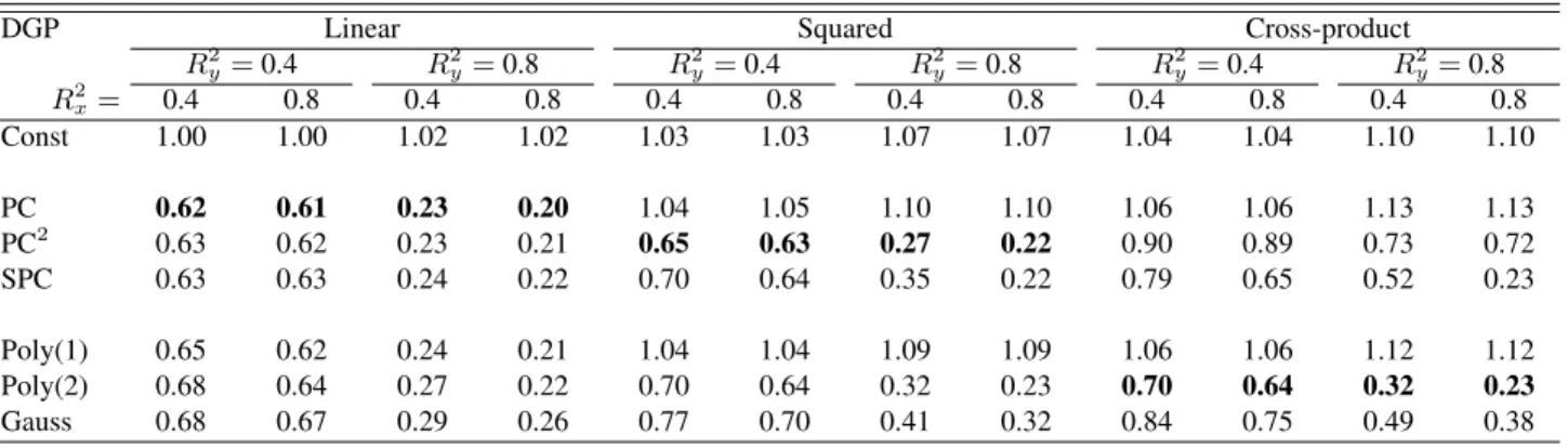
Table 1 shows mean squared prediction errors relative to the variance of the series being predicted. Note that if the factor valuesf1,T+1andf2,T+1were known, these relative MSPEs would be close to1−R2y, or 0.6
and 0.2 in the two scenarios of “weak” (Ry2 = 0.4) and “strong” (R2y = 0.8) predictive structure considered here. Standard PC shows good performance for the linear DGP, and PC2 for the squared DGP. Such results are to be expected, because the forecast equation in these methods corresponds exactly with these DGPs. Interestingly, the kernel methods are not much less accurate than these “optimal” methods, with the obvious exception of the Poly(1) (that is, linear) kernel in the squared DGP (for which standard PC also fares badly). This finding holds regardless of whetherR2
xandR2y are high or low, although the difference between PC or
Table 1:Relative Mean Squared Prediction Errors for the Factor Models (5)-(7).
DGP Linear Squared Cross-product
R2y=0.4 R2y=0.8 R2y=0.4 R2y=0.8 R2y=0.4 R2y=0.8 R2x= 0.4 0.8 0.4 0.8 0.4 0.8 0.4 0.8 0.4 0.8 0.4 0.8 Const 1.00 1.00 1.02 1.02 1.03 1.03 1.07 1.07 1.04 1.04 1.10 1.10 PC 0.62 0.61 0.23 0.20 1.04 1.05 1.10 1.10 1.06 1.06 1.13 1.13 PC2 0.63 0.62 0.23 0.21 0.65 0.63 0.27 0.22 0.90 0.89 0.73 0.72 SPC 0.63 0.63 0.24 0.22 0.70 0.64 0.35 0.22 0.79 0.65 0.52 0.23 Poly(1) 0.65 0.62 0.24 0.21 1.04 1.04 1.09 1.09 1.06 1.06 1.12 1.12 Poly(2) 0.68 0.64 0.27 0.22 0.70 0.64 0.32 0.23 0.70 0.64 0.32 0.23 Gauss 0.68 0.67 0.29 0.26 0.77 0.70 0.41 0.32 0.84 0.75 0.49 0.38 NOTE: This table reports mean squared prediction errors (MSPEs) for models (5)-(7), averaged over 5000 forecasts, and relative to the variance of the series being predicted. The smallest relative MSPE for each DGP (column) is printed in boldface.
stronger (compareR2x = 0.4withR2x = 0.8). Thus, we find that kernel methods can work well in standard factor model settings.
For the cross-product DGP, the SPC method from Bai and Ng (2008) and the Poly(2) kernel can both be expected to perform well. We observe that kernel ridge regression provides the most accurate forecasts here, and that the gains are larger for lowerR2x. Thus kernel ridge regression performs well in this case, especially when the factor structure of the predictors is not very strong, as is often the case for empirical macroeconomic and financial data. The performance of the Gaussian kernel is also satisfactory.
We conclude that the use of kernel methods in a factor context works quite well, especially for nonlinear relations, and in situations where the observed predictors give relatively little information on the factors.
4
MACROECONOMIC FORECASTING
4.1 Data and Forecast Models
To evaluate the forecast performance of kernel ridge regression in an empirical application, we consider fore-casting of four key macroeconomic variables. The data set consists of monthly observations on 132 U.S. macroeconomic variables, including various measures of production, consumption, income, sales, employ-ment, monetary aggregates, prices, interest rates, and exchange rates. All series have been transformed to
stationarity by taking logarithms and/or differences, as described in Stock and Watson (2005). We have up-dated their data set, which starts in January 1959 and ends in December 2003, to cover the period until (and including) January 2010. The cross-sectional dimension varies somewhat because of data availability: some time series start later than January 1959, while a few other variables have been discontinued before the end of our sample period. For each month under consideration, observations on at most five variables are missing.
We focus on forecasting four key measures of real economic activity: Industrial Production, Personal Income, Manufacturing & Trade Sales, and Employment. (The acronyms by which Stock and Watson (2002) refer to these series areip, gmyxpq, msmtq, and lhnag, respectively.) For each of these variables, we produce out-of-sample forecasts for the annualizedh-month percentage growth rate, computed as
yth+h= 1200 h ln vt+h vt ,
wherevtis the untransformed observation on the level of each variable in montht. To simplify notation, we
denote the one-month growth rate asyt+1. We consider growth rate forecasts forh= 1,3,6and 12 months.
The kernel ridge forecasts are compared against several alternative forecasting approaches that are pop-ular in current macroeconomic practice. As benchmarks we include (i) the constant forecast (that is, the average growth over the estimation window); (ii) the no-change (that is, random-walk) forecast; and (iii) an autoregressive forecast. In addition, as the primary competitor for kernel methods we consider the diffusion index (DI) approach of Stock and Watson (2002), who document its good performance for forecasting these four macroeconomic variables. The DI methodology extends the standard principal component regression by including autoregressive lags as well as lags of the principal components in the forecast equation. Specif-ically, usingpautoregressive lags and q lags of k factors, at timet, this “extended” principal-components method produces the forecast
ˆ yth+h|t=wt0βˆ+ ˆft0ˆγ, wherewt = 1, yt, yt−1. . . , yt−(p−1) 0 andfˆt = ˆ f1,t,fˆ2,t, . . . ,fˆk,t,fˆ1,t−1, . . . ,fˆk,t−(q−1) 0 . The lags of the dependent variable inwt are one-month growth rates, irrespective of the forecast horizon h, because
components extracted from all 132 predictor variables, andβˆandˆγare OLS estimates. Aside from standard principal components (PC), we also consider its extensions PC2 and SPC, discussed in Section 3. In each case, the lag lengthspandqand the number of factorskare selected by minimizing the Bayesian Information Criterion (BIC). This criterion is used instead of cross-validation for two reasons. We want our results to be comparable to those in Stock and Watson (2002) and Bai and Ng (2008), and preliminary experimentation has revealed that using the BIC leads to superior results. Like Stock and Watson (2002), we allow0≤p≤6,
1≤q ≤3, and1 ≤k≤4; thus, the simplest model that can be selected uses no information on current or lagged values of the dependent variable, and information from the other predictors in the current month only, summarized by one factor. In line with Stock and Watson (2002), we do not perform an exhaustive search across all possible combinations of the first four principal components and lag structures. Instead, we assume that factors are included sequentially in order of importance, while the number of lags is assumed to be the same for all included factors.
For kernel ridge regression, the corresponding forecast equation is
ˆ yth+h|t=wt0βˆ+ϕ x0t, x0t−1, . . . , x0t−(q−1) 00 ˆ γ,
in the notation of Section 2.2, wherewtis as defined above andxtcontains all 132 predictors at timet. The
parameter vectorsβˆandγˆare obtained by kernel ridge regression, resulting in the forecast equation (2). The lag lengthspandq, as well as the kernel penalty parameterλ, are selected by leave-one-out cross-validation. All models are estimated on rolling windows with a fixed length of 120 months, such that the first forecast is produced for the growth rate during the firsth months of 1970. For each window, the tuning parameter values are re-selected and the regression coefficients are re-estimated. That is, all of the tuning parameters (p, q, k, λ) are allowed to differ over time and across methods.
4.2 Results
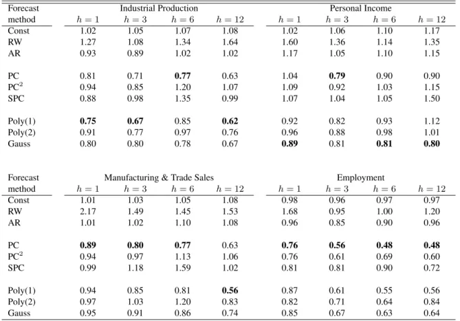
Table 2 shows the mean squared prediction errors (MSPEs) for the period 1970-2010 for three simple bench-mark methods, three PC-based methods, and three kernel methods. Several conclusions can be drawn from these results. We first observe that kernel ridge regression provides more accurate forecasts than any of the
Table 2:Relative Mean Squared Prediction Errors for the Macroeconomic Series.
Forecast Industrial Production Personal Income
method h= 1 h= 3 h= 6 h= 12 h= 1 h= 3 h= 6 h= 12 Const 1.02 1.05 1.07 1.08 1.02 1.06 1.10 1.17 RW 1.27 1.08 1.34 1.64 1.60 1.36 1.14 1.35 AR 0.93 0.89 1.02 1.02 1.17 1.05 1.10 1.15 PC 0.81 0.71 0.77 0.63 1.04 0.79 0.90 0.90 PC2 0.94 0.85 1.20 1.07 1.09 0.92 1.03 1.15 SPC 0.88 0.98 1.35 0.99 1.07 1.04 1.05 1.50 Poly(1) 0.75 0.67 0.85 0.62 0.92 0.82 0.93 1.12 Poly(2) 0.91 0.77 0.97 0.76 0.96 0.88 0.98 1.01 Gauss 0.80 0.80 0.78 0.67 0.89 0.81 0.81 0.80
Forecast Manufacturing & Trade Sales Employment
method h= 1 h= 3 h= 6 h= 12 h= 1 h= 3 h= 6 h= 12 Const 1.01 1.03 1.05 1.08 0.98 0.96 0.97 0.97 RW 2.17 1.49 1.45 1.53 1.68 0.95 1.00 1.20 AR 1.01 1.02 1.10 1.08 0.96 0.85 0.90 0.96 PC 0.89 0.80 0.77 0.63 0.76 0.56 0.48 0.48 PC2 0.94 0.97 1.13 1.06 0.76 0.61 0.69 0.60 SPC 0.99 1.18 1.59 1.02 0.81 0.81 0.90 0.72 Poly(1) 0.94 0.85 0.81 0.56 0.87 0.61 0.55 0.56 Poly(2) 0.97 1.03 1.20 0.83 0.82 0.71 0.64 0.84 Gauss 0.95 0.91 0.86 0.74 0.85 0.67 0.63 0.64
NOTE: This table reports mean squared prediction errors (MSPEs) for four macroeconomic series, over the period 1970-2010, relative to the variance of the series being predicted. The smallest relative MSPE for each series (column) is printed in boldface.
three benchmarks (constant, random walk, and autoregression) for all of the target variables and all forecast horizons, with larger gains for longer horizons. This holds irrespective of the kernel function that is used, the only exceptions being that the second-order polynomial kernel produces worse forecasts for the three-month and six-month growth rates of Manufacturing & Trade Sales. In many cases the improvements in predictive accuracy are substantial, even compared to the AR forecast, which seems the best of the three benchmarks. For example, for 12-month growth rate forecasts, the kernel ridge regression based on the Gaussian kernel achieves a reduction in MSPE of about 30% for all four variables.
Second, if we compare the forecasts based on kernel ridge regression and the linear PC-based approach, we find somewhat mixed results, but generally the kernel methods perform better. Kernel ridge forecasts are
superior for Industrial Production and Personal Income. For Manufacturing & Trade Sales, kernels perform better at the longest horizon and slightly worse at the shorter horizons. Finally, for Employment, the PC-based forecasts are more accurate than kernel-based forecasts.
Third, the kernel ridge regression approach convincingly outperforms the PC2 and SPC variants of the principal component regression framework. In fact, also the linear PC specification clearly outperforms these two extensions in all cases. Apparently, the PC2and SPC methods cannot successfully cope with the possibly nonlinear relations between the target variables and the predictors in this application. (Bai and Ng (2008) report somewhat better performance if SPC is applied to a selected subset of the predictors, rather than to the full predictor set. Also with this modification, SPC has difficulties outperforming simpler linear methods.)
Fourth, among the kernel-based methods, the Poly(1) kernel and the Gaussian kernel generally perform best. All but one of the MSPE / variance ratios in Table 2 are below one for these methods. Neither of the two consistently outperforms the other. Although Poly(1) performs better than the Gaussian kernel in some cases, the latter kernel method shows satisfactory results in all situations.
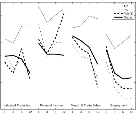
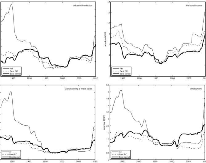
A subset of the results in Table 2 is reproduced graphically in Figure 1. This graph allows us to interpret the mixed results in the comparison of kernel-based and linear PC-based forecasts as follows. Kernel ridge regression (especially using the Gaussian kernel) shows roughly the same good performance for all four se-ries, but the quality of PC forecasts varies among the series and is exceptionally high for the Employment series. Recall that in the Monte Carlo experiment in Section 3, we find the analogous result that kernel-based methods yield better relative performance, compared to PC-based methods, if the factor structure is relatively weak. That is, our results suggest that kernel ridge regression performs better than principal component re-gression unless the latter performs very well. To further investigate this idea, Figure 2 shows time-series plots of rolling mean squared prediction errors. The value plotted for datetis the mean squared prediction error (without correcting for the variance of the predicted series) computed over the ten-year subsample ending with the forecast for datet, that is,yˆth|t−h. We show only the series forh = 12, as the results for the other horizons are qualitatively similar. This figure confirms that, when kernel-based forecasts are less accurate than PC-based forecasts, this is because PC-based forecasts are very accurate, and not because kernel-based forecasts would be inaccurate. Another interesting feature evidenced by Figure 2 is that, although the recent
1 3 6 12 1 3 6 12 1 3 6 12 1 3 6 12 0.4 0.5 0.6 0.7 0.8 0.9 1 1.1 1.2
Forecast horizon (months)
Relative MSPE
Industrial Production Personal Income Manuf. & Trade Sales Employment
AR PC Poly(1) Gauss
Figure 1:Relative Mean Squared Prediction Errors for Four Macroeconomic Series, for selected methods.
crisis reduces the accuracy of all forecasts from 2008 onward, if affects the kernel-based forecasts least. Following Stock and Watson (2002), we provide a further evaluation of our results by using the forecast combining regression
yth+h =αyˆth+h|t+ (1−α) ˆyth,+ARh|t+uht+h, (8) whereyth+his the realized growth rate over theh-month period ending in montht+h,yˆth+h|tis a candidate forecast from either the PC-based methods or from kernel ridge regression made at time t, and yˆth,+ARh|t is the benchmark autoregressive forecast. Estimates of α are shown in Table 3, with heteroscedasticity and autocorrelation consistent (HAC) standard errors in parentheses. The null hypothesis that the AR forecast receives unit weight (α= 0) is strongly rejected in almost all cases, which means that PC-based and kernel-based forecasts have significant additional predictive ability relative to this benchmark. Actually, the null hypothesis that the candidate forecast receives unit weight (α = 1) cannot be rejected in many cases. If
α = 1, this means that the candidate forecast encompasses the AR forecast. This hypothesis is not rejected for PC-based methods in 17 out of 48 cases, and for kernel-based methods even in 37 out of 48 cases.
1985 1990 1995 2000 2005 2010 0 5 10 15 20 25 30 35 40 45 50 Absolute MSPE Industrial Production AR Best PC Best kernel 1985 1990 1995 2000 2005 2010 0 2 4 6 8 10 12 14 Absolute MSPE Personal Income AR Best PC Best kernel 1985 1990 1995 2000 2005 2010 0 5 10 15 20 25 30 35 40 45 50 Absolute MSPE
Manufacturing & Trade Sales
AR Best PC Best kernel 1985 1990 1995 2000 2005 2010 0 0.5 1 1.5 2 2.5 3 3.5 4 4.5 5 5.5 Absolute MSPE Employment AR Best PC Best kernel
Figure 2:Ten-Year Rolling-Window Mean Squared Prediction Errors for Four Macroeconomic Series, for a forecast horizon ofh= 12months, for AR and for the best-performing PC and kernel methods.
In order to compare the performance of kernel-based and PC-based forecasts directly, we run a similar forecast combining regression
yth+h =αyˆth,+kernelh|t + (1−α) ˆyh,t+PCh|t+uht+h. (9) As linear PC performs better than PC2and SPC (see Table 2), we compare kernel methods to linear PC only. We report the estimates ofαin Table 4. These results show that both hypotheses of interest (α= 0andα= 1) are rejected in many cases (26 out of 48), suggesting that forecasts obtained from both types of models are complementary. Apparently, each forecast method uses relevant information that the other method misses.
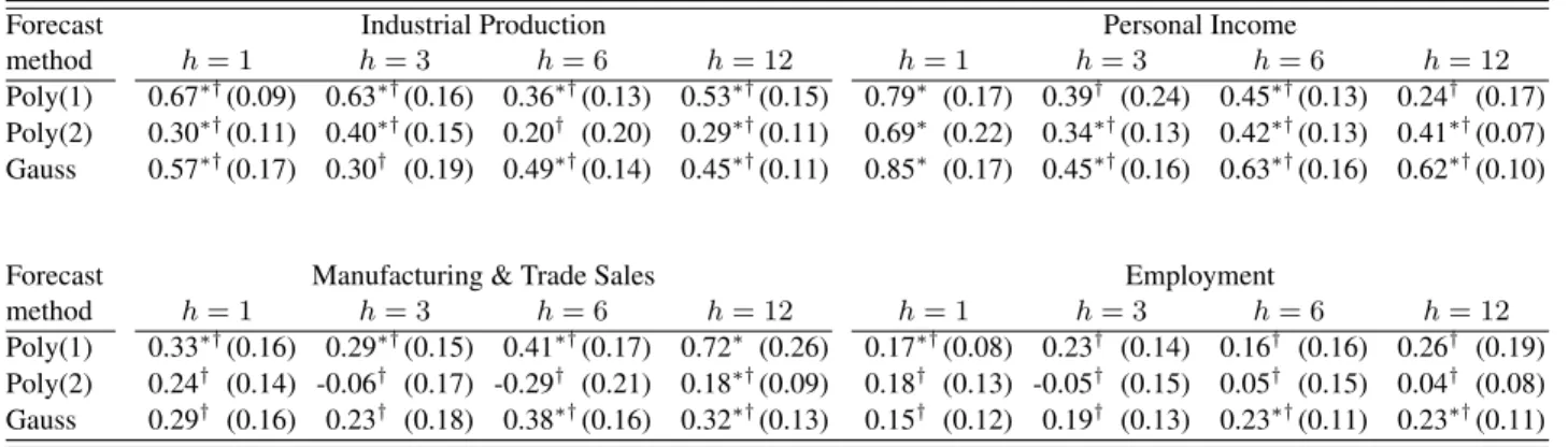
Table 3:Estimated Coefficientsαˆfrom the Forecast Combining Regression (8).
Forecast Industrial Production Personal Income
method h= 1 h= 3 h= 6 h= 12 h= 1 h= 3 h= 6 h= 12 PC 0.83∗ (0.15) 0.80∗ (0.14) 0.72∗†(0.13) 0.79∗ (0.11) 0.97∗ (0.26) 0.87∗ (0.12) 0.70∗†(0.10) 0.70∗†(0.09) PC2 0.48∗†(0.15) 0.55∗†(0.11) 0.42∗†(0.12) 0.48∗†(0.13) 0.71∗ (0.18) 0.66∗†(0.12) 0.54∗†(0.07) 0.50∗†(0.10) SPC 0.57∗†(0.08) 0.43∗†(0.11) 0.37∗†(0.12) 0.51∗†(0.08) 0.75∗ (0.21) 0.51∗†(0.09) 0.52∗†(0.10) 0.39∗†(0.08) Poly(1) 0.89∗ (0.11) 0.91∗ (0.14) 0.63∗†(0.13) 0.81∗ (0.12) 1.07∗ (0.19) 1.01∗ (0.14) 0.63∗†(0.12) 0.52∗†(0.12) Poly(2) 0.53∗†(0.09) 0.77∗ (0.19) 0.55∗ (0.25) 0.85∗ (0.15) 1.01∗ (0.23) 0.78∗ (0.14) 0.63∗†(0.15) 0.68∗ (0.17) Gauss 1.23∗ (0.18) 0.74∗ (0.16) 0.89∗ (0.15) 0.99∗ (0.17) 1.29∗†(0.14) 1.10∗ (0.15) 0.96∗ (0.15) 0.95∗ (0.14)
Forecast Manufacturing & Trade Sales Employment
method h= 1 h= 3 h= 6 h= 12 h= 1 h= 3 h= 6 h= 12 PC 0.83∗ (0.12) 0.86∗ (0.13) 0.87∗ (0.17) 0.91∗ (0.12) 1.02∗ (0.09) 0.93∗ (0.09) 0.92∗ (0.10) 1.04∗ (0.12) PC2 0.64∗†(0.08) 0.55∗†(0.11) 0.48∗†(0.19) 0.51∗†(0.15) 0.91∗ (0.06) 0.74∗†(0.07) 0.62∗†(0.10) 0.77∗ (0.14) SPC 0.53∗†(0.09) 0.39∗†(0.14) 0.29† (0.15) 0.52∗†(0.10) 0.74∗†(0.07) 0.53∗†(0.08) 0.50∗†(0.09) 0.60∗†(0.09) Poly(1) 0.66∗†(0.14) 0.83∗ (0.18) 0.80∗ (0.16) 0.97∗ (0.15) 0.68∗†(0.12) 0.97∗ (0.14) 0.97∗ (0.11) 0.91∗ (0.14) Poly(2) 0.61∗†(0.12) 0.48∗†(0.17) 0.40† (0.24) 0.89∗ (0.26) 0.90∗ (0.11) 0.74∗ (0.21) 0.77∗ (0.13) 0.66∗ (0.19) Gauss 0.76∗ (0.13) 0.89∗ (0.17) 0.86∗ (0.14) 1.06∗ (0.22) 0.98∗ (0.15) 1.21∗ (0.18) 1.10∗ (0.13) 1.07∗ (0.18) NOTE: This table reportsαˆ, the weight placed on the candidate forecast in the forecast combining regression (8). HAC standard errors follow in parentheses. An asterisk (∗) indicates rejection of the hypothesisα= 0and a dagger (†) indicates rejection ofα= 1, at the5%significance level.
Table 4:Estimated Coefficientsαˆfrom the Forecast Combining Regression (9).
Forecast Industrial Production Personal Income
method h= 1 h= 3 h= 6 h= 12 h= 1 h= 3 h= 6 h= 12
Poly(1) 0.67∗†(0.09) 0.63∗†(0.16) 0.36∗†(0.13) 0.53∗†(0.15) 0.79∗ (0.17) 0.39† (0.24) 0.45∗†(0.13) 0.24† (0.17) Poly(2) 0.30∗†(0.11) 0.40∗†(0.15) 0.20† (0.20) 0.29∗†(0.11) 0.69∗ (0.22) 0.34∗†(0.13) 0.42∗†(0.13) 0.41∗†(0.07) Gauss 0.57∗†(0.17) 0.30† (0.19) 0.49∗†(0.14) 0.45∗†(0.11) 0.85∗ (0.17) 0.45∗†(0.16) 0.63∗†(0.16) 0.62∗†(0.10)
Forecast Manufacturing & Trade Sales Employment
method h= 1 h= 3 h= 6 h= 12 h= 1 h= 3 h= 6 h= 12
Poly(1) 0.33∗†(0.16) 0.29∗†(0.15) 0.41∗†(0.17) 0.72∗ (0.26) 0.17∗†(0.08) 0.23† (0.14) 0.16† (0.16) 0.26† (0.19) Poly(2) 0.24† (0.14) -0.06† (0.17) -0.29† (0.21) 0.18∗†(0.09) 0.18† (0.13) -0.05† (0.15) 0.05† (0.15) 0.04† (0.08) Gauss 0.29† (0.16) 0.23† (0.18) 0.38∗†(0.16) 0.32∗†(0.13) 0.15† (0.12) 0.19† (0.13) 0.23∗†(0.11) 0.23∗†(0.11) NOTE: This table reportsαˆ, the weight placed on the kernel-based forecast in the forecast combining regression (9). HAC standard errors follow in parentheses. An asterisk (∗) indicates rejection of the hypothesisα= 0and a dagger (†) indicates rejection ofα= 1, at the5%significance level.
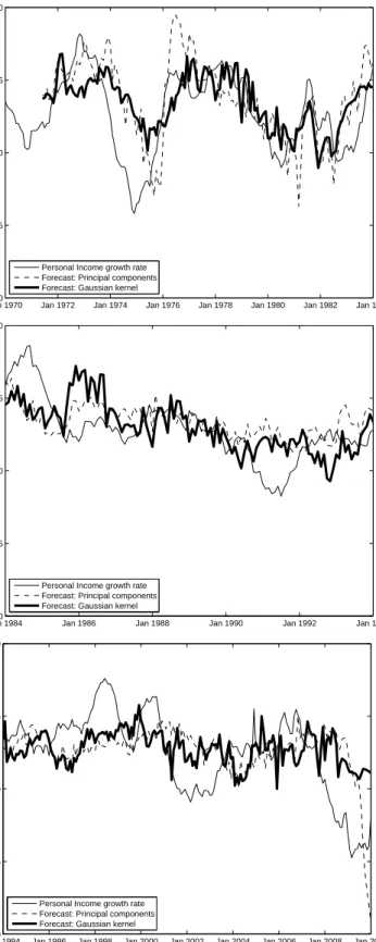
Jan 1970 Jan 1972 Jan 1974 Jan 1976 Jan 1978 Jan 1980 Jan 1982 Jan 1984 −10 −5 0 5 10
Personal Income growth rate Forecast: Principal components Forecast: Gaussian kernel
Jan 1984 Jan 1986 Jan 1988 Jan 1990 Jan 1992 Jan 1994 −10
−5 0 5 10
Personal Income growth rate Forecast: Principal components Forecast: Gaussian kernel
Jan 1994 Jan 1996 Jan 1998 Jan 2000 Jan 2002 Jan 2004 Jan 2006 Jan 2008 Jan 2010 −10
−5 0 5 10
Personal Income growth rate Forecast: Principal components Forecast: Gaussian kernel
Finally, we show time series plots of the twelve-month growth rate of Personal Income in Figure 3. The choice of the three subperiods is motivated by dating the Great Moderation in 1984. The first subperiod con-tains only pre-Moderation data. As we estimate all models on 120-month rolling windows, the first forecast that is based only on post-Moderation data is the one for 1994, which marks the start of the last subperiod. During the second subperiod (see the middle panel of Figure 3), the kernel-based forecast is much more volatile than both the actual time series and the PC-based forecast. Apparently, kernel ridge regression is relatively more heavily affected by the break in volatility in the Personal Income series at the Great Modera-tion (with a variance of 7.84 for 1970-1983 and of 6.53 for 1984-2010). On both other subsamples, however, allowing for nonlinearity through kernel methods enhances the forecast quality considerably, see the top and bottom panels of Figure 3. The relative MSPEs, compared to the AR benchmark, for the three subperiods 1970-1983, 1984-1993, and 1994-2010 are respectively 86%, 71%, and 76% for PC, as compared to 70%, 77%, and 67% for Gaussian kernel ridge regression. This result shows that the kernel method performs bet-ter than PC in the first and last subperiod. We also note the “overshooting” of the 2008-9 crisis by the PC forecasts in the bottom panel of Figure 3. This does not occur for kernel ridge regression, as such extreme forecasts are suppressed by the shrinkage parameter.
5
CONCLUSION
We have introduced kernel ridge regression as a framework for estimating nonlinear predictive relations in a data-rich environment. We have extended the existing kernel methodology to enable its use in time-series contexts typical for macroeconomic and financial applications. These extensions involve the incorporation of unpenalized linear terms in the forecast equation and an efficient leave-one-out cross-validation procedure for model selection purposes. Our simulation study suggests that this method can deal with the type of data that comes up frequently in economic analysis, namely, data with a factor structure.
The empirical application to forecasting four key U.S. macroeconomic variables — production, income, sales, and employment — shows that kernel-based methods are often preferable to, and always competitive with, well-established autoregressive and principal-components-based methods. Kernel techniques also out-perform previously proposed extensions of the standard PC-based approach to accommodate nonlinearity.
Kernel ridge regression exhibits a relatively consistent good predictive performance, also during the crisis period in 2008-9. It is outperformed by linear principal components only in those periods when the latter method performs exceptionally well. Among the kernel methods, linear and Gaussian kernels are found to produce the most reliable forecasts, and neither of these two kernels consistently outperforms the other. This finding implies that the ridge term contributes importantly to the predictive accuracy, while accounting for nonlinearity also helps in many cases. As using the Gaussian kernel does not require the forecaster to specify the form of nonlinearity in advance, this method is a powerful tool.
Finally, we have provided statistical evidence that kernel-based forecasts contain information that principal-components-based forecasts miss, and vice versa. This result suggests a potential for forecast combination techniques. We conclude that the kernel methodology is a valuable addition to the macroeconomic fore-caster’s toolkit.
APPENDIX: TECHNICAL RESULTS
This appendix contains derivations of three results stated in Section 2: the expression for the forecast equation (2) for kernel ridge regression with additional unpenalized linear terms, the expansion of the Gaussian kernel, and the leave-one-out cross-validation method that we use for selecting tuning parameters.
A.1 Kernel Ridge Regression with Unpenalized Linear Terms (Section 2.2)
We have shown in Section 2.2 that minimization of the penalized least-squares criterion||y−Zγ||2+λ||γ||2
leads to the forecasty∗ˆ =k∗0 (K+λI)−1y; this is Equation (1) in Section 2.2. In this appendix, we modify this forecast equation to allow for unpenalized linear terms. That is, we seek to minimize
||y−W β−Zγ||2+λ||γ||2 (10) over theP ×1vectorβand theM×1vectorγ. For givenβˆ, we can proceed as in Section 2.2; we find
ˆ γ =Z0(K+λI)−1 y−Wβˆ . (11)
On the other hand, for givenγˆ, minimizing criterion (10) is equivalent to ordinary least squares regression:
ˆ
β = W0W−1
W0(y−Zγˆ). (12)
We substitute the expression forˆγfrom Equation (11) into Equation (12), recall thatK =ZZ0, and rearrange the resulting equation to obtain
W0I−K(K+λI)−1Wβˆ = W0I−K(K+λI)−1y W0(K+λI−K) (K+λI)−1Wβˆ = W0(K+λI−K) (K+λI)−1y
ˆ β = W0(K+λI)−1W −1 W0(K+λI)−1y.
If we substitute this result and Equation (11) into the forecast equationy∗ˆ = z∗0ˆγ +w∗0βˆ, and recall that
k∗ =Zz∗, we find ˆ y∗ = k0∗(K+λI)−1 I−W W0(K+λI)−1W −1 W0(K+λI)−1 y +w0∗W0(K+λI)−1W −1 W0(K+λI)−1y. (13)
To obtain a more manageable equation, recall that the partitioned matrix inverse
K+λI W W0 0 −1 equals (K+λI)−1 I−W W0(K+λI)−1W−1W0(K+λI)−1 (K+λI)−1WW0(K+λI)−1W−1 W0(K+λI)−1W −1 W0(K+λI)−1 −W0(K+λI)−1W −1 . (14) It follows from this result that Equation (13) is equivalent to Equation (2) in Section 2.2:
ˆ y∗ = k∗ w∗ 0 K+λI W W0 0 −1 y 0 .
A.2 Expansion of the Gaussian Kernel (Section 2.3)
In this appendix, we derive the mappingϕthat corresponds to the Gaussian kernel function. As stated in Equation (4) in Section 2.3, this kernel function is defined asκ(a, b) = exp
−(1/2)||a−b||2. If we write
−(1/2)||a−b||2 =−a0a/2−b0b/2 +a0band expand the Taylor series forexp (a0b), we obtain
κ(a, b) =e−a0a/2e−b0b/2 ∞ X r=0 1 r! a 0br . (15)
We proceed by expanding(a0b)ras a multinomial series:
a0br= N X n=1 anbn !r = X X· · ·X {PN n=1dn=r,alldn≥0} r! QN n=1dn! N Y n=1 (anbn)dn ! .
Substituting this result into Equation (15), we find
κ(a, b) = e−a0a/2e−b0b/2 ∞ X r=0 1 r! X X · · ·X {PN n=1dn=r,alldn≥0} r! QN n=1dn! N Y n=1 (anbn)dn ! = e−a0a/2e−b0b/2 ∞ X r=0 X X · · ·X {PN n=1dn=r,alldn≥0} N Y n=1 (anbn)dn dn! ! = e−a0a/2e−b0b/2 X X· · ·X {alldn≥0,forn=1,2,...,N} N Y n=1 (anbn)dn dn! ! .
Finally, we split the product into two factors that depend only onaand only onb, respectively:
κ(a, b) = ∞ X d1=0 ∞ X d2=0 · · · ∞ X dN=0 e−a0a/2 N Y n=1 adn n √ dn! ! e−b0b/2 N Y n=1 bdn n √ dn! ! . (16)
As expression (16) shows, κ(a, b) = ϕ(a)0ϕ(b), where, as claimed in Section 2.3, ϕ(a) contains as ele-ments, for each combination of degreesd1, d2, . . . , dN ≥0,
e−a0a/2 N Y n=1 adn n √ dn! .
A.3 Computationally Efficient Leave-One-Out Cross-Validation (Section 2.4)
In this appendix, we describe an efficient method for leave-one-out cross-validation. Our derivation extends the results in Cawley and Talbot (2008) to allow for the unpenalized linear terms in the forecast equation (2). The result of Appendix A.1 can be summarized as follows: kernel ridge regression leads to the forecast
ˆ y∗ = k∗ w∗ 0 ˆ α ˆ β with K+λI W W0 0 ˆ α ˆ β = y 0 . (17)
The first step in leave-one-out cross-validation is to estimate the model on all observations except the first. AsK =ZZ0, and each row ofZ depends only on the corresponding row ofX, the only elements inKthat depend on the first observation are those in the first row and those in the first column. We therefore separate the first row and column from the other elements ofK, and likewise, we split off the first row ofW, the first element ofαˆ, and the first element ofy. We denote these partitioned matrices and vectors by
K= k1,1 k0−1,1 k−1,1 K−1,−1 , W = w10 W−1 , αˆ= ˆ α1 ˆ α−1 and y= y1 y−1 .
We then have, from Equation (17),
k1,1+λ k−0 1,1 w10 k−1,1 K−1,−1+λI W−1 w1 W−01 0 ˆ α1 ˆ α−1 ˆ β = y1 y−1 0 ,
or equivalently, separating the first equation from the others,
ˆ α1(k1,1+λ) + k−1,1 w1 0 ˆ α−1 ˆ β = y1, (18) ˆ α1 k−1,1 w1 + K−1,1+λI W−1 W−01 0 ˆ α−1 ˆ β = y−1 0 . (19)
The forecast ofy1based on a model estimated on observations2,3, . . . , T clearly equals ˜ y1 = k−1,1 w1 0 K−1,−1+λI W−1 W−01 0 −1 y−1 0
and we may write
˜ y1 = αˆ1 k−1,1 w1 0 K−1,−1+λI W−1 W−01 0 −1 k−1,1 w1 + k−1,1 w1 0 ˆ α−1 ˆ β using Equation (19) = αˆ1 k−1,1 w1 0 K−1,−1+λI W−1 W−01 0 −1 k−1,1 w1 +y1−αˆ1(k1,1+λ) using Equation (18) = y1−αˆ1 k1,1+λ− k−1,1 w1 0 K−1,−1+λI W−1 W−01 0 −1 k−1,1 w1 . The expressionk1,1+λ− k−1,1 w1 0 K−1,−1+λI W−1 W−01 0 −1 k−1,1 w1
equals the reciprocal of
element(1,1)of k1,1+λ k0−1,1 w01 k−1,1 K−1,−1+λI W−1 w1 W−01 0 −1 = K+λI W W0 0 −1
, as can be seen by using
the partitioned matrix inversion formula. Therefore, the first leave-one-out error equals
y1−y˜1 = ˆα1 , element (1,1) of K+λI W W0 0 −1 .
In general, an analogous calculation shows that thetth leave-one-out prediction error equals
yt−y˜t= ˆαt , element (t, t) of K+λI W W0 0 −1 . (20)
That is, we can compute all leave-one-out errors by dividing each element of the vectorαˆby the corresponding diagonal element of the matrix
K+λI W W0 0 −1
. Observe that bothαˆand this matrix inverse are needed in computing the out-of-sample forecasty∗ˆ . Thus, in the process of making the out-of-sample prediction, we can find all leave-one-out errors without performing any additional computations, aside from the division in Equation (20).
As a final note, we mention that the matrix inverse in Equation (20) can also be computed efficiently. As
K+λI is symmetric and positive definite, its inverse can be computed from its Cholesky decomposition. The inverse of the full matrix can then be calculated using Equation (14) in Appendix A.1.
REFERENCES
Aiolfi, M. and Favero, C. A. (2005), “Model Uncertainty, Thick Modelling and The Predictability of Stock Returns,”Journal of Forecasting, 24, 233–254.
Bai, J. and Ng, S. (2008), “Forecasting Economic Time Series Using Targeted Predictors,”Journal of Econo-metrics, 146, 304–317.
Boser, B. E., Guyon, I. M., and Vapnik, V. M. (1992), “A Training Algorithm for Optimal Margin Classifiers,” inProceedings of the Annual Conference on Computational Learning Theory, ed. Haussler, D., Pittsburgh, Pennsylvania: ACM Press, pp. 144–152.
Broomhead, D. S. and Lowe, D. (1988), “Multivariable Functional Interpolation and Adaptive Networks,”
Complex Systems, 2, 321–355.
Cawley, G. C. and Talbot, N. L. C. (2008), “Efficient Approximate Leave-One-Out Cross-Validation for Kernel Logistic Regression,”Machine Learning, 71, 243–264.
C¸ akmaklı, C. and van Dijk, D. (2010), “Getting the Most out of Macroeconomic Information for Predicting Stock Returns and Volatility,”Tinbergen Institute Discussion Paper 2010-115/4.
De Mol, C., Giannone, D., and Reichlin, L. (2008), “Forecasting Using a Large Number of Predictors: Is Bayesian Shrinkage a Valid Alternative to Principal Components?” Journal of Econometrics, 146, 318– 328.
Faust, J. and Wright, J. H. (2009), “Comparing Greenbook and Reduced Form Forecasts Using a Large Realtime Dataset,”Journal of Business and Economic Statistics, 27, 468–479.
Groen, J. J. J. and Kapetanios, G. (2008), “Revisiting Useful Approaches to Data-Rich Macroeconomic Forecasting,”Federal Reserve Bank of New York Staff Report 327.
Huang, H. and Lee, T.-H. (2010), “To Combine Forecasts or to Combine Information?”Econometric Reviews, 29, 534–570.
Ludvigson, S. C. and Ng, S. (2007), “The Empirical Risk-Return Relation: A Factor Analysis Approach,”
Journal of Financial Economics, 83, 171–222.
— (2009), “Macro Factors in Bond Risk Premia,”Review of Financial Studies, 22, 5027–5067.
Medeiros, M. C., Ter¨asvirta, T., and Rech, G. (2006), “Building Neural Network Models for Time Series: A Statistical Approach,”Journal of Forecasting, 25, 49–75.
M¨uller, K.-R., Smola, A., R¨atsch, G., Sch¨olkopf, B., Kohlmorgen, J., and Vapnik, V. (1997), “Predicting Time Series with Support Vector Machines,” inArtificial Neural Networks ICANN’97, eds. Gerstner, W., Germond, A., Hasler, M., and Nicoud, J.-D., Berlin: Springer, pp. 999–1004.
Pagan, A. R. and Ullah, A. (1999),Nonparametric Econometrics, Cambridge, United Kingdom: Cambridge University Press.
Poggio, T. (1975), “On Optimal Nonlinear Associative Recall,”Biological Cybernetics, 19, 201–209. Racine, J. (2000), “Consistent Cross-Validatory Model-Selection for Dependent Data: hv-Block
Cross-Validation,”Journal of Econometrics, 99, 39–61.
Rapach, D. E., Strauss, J. K., and Zhou, G. (2010), “Out-of-Sample Equity Premium Prediction: Combination Forecasts and Links to the Real Economy,”Review of Financial Studies, 23, 821–862.
Sch¨olkopf, B., Smola, A., and M¨uller, K.-R. (1998), “Nonlinear Component Analysis as a Kernel Eigenvalue Problem,”Neural Computation, 10, 1299–1319.
Smola, A. J. and Sch¨olkopf, B. (2004), “A Tutorial on Support Vector Regression,”Statistics and Computing, 14, 199–222.
Stock, J. H. and Watson, M. W. (1999), “A Comparison of Linear and Nonlinear Univariate Models for Forecasting Macroeconomic Time Series,” in Cointegration, Causality and Forecasting. A Festschrift in Honour of Clive W. J. Granger, eds. Engle, R. F. and White, H., Oxford: Oxford University Press, pp. 1–44.
— (2002), “Macroeconomic Forecasting Using Diffusion Indexes,”Journal of Business and Economic Statis-tics, 20, 147–162.
— (2005), “Implications of Dynamic Factor Models for VAR Analysis,”NBER Working Paper No. 11467. — (2006), “Forecasting with Many Predictors,” in Handbook of Economic Forecasting, eds. Elliot, G.,
Granger, C. W. J., and Timmermann, A., Amsterdam: Elsevier, pp. 515–554.
— (2009), “Generalized Shrinkage Methods for Forecasting Using Many Predictors,”Manuscript, Harvard University.
Ter¨asvirta, T. (2006), “Forecasting Economic Variables with Nonlinear Models,” inHandbook of Economic Forecasting, eds. Elliot, G., Granger, C. W. J., and Timmermann, A., Amsterdam: Elsevier, pp. 413–458. Ter¨asvirta, T., van Dijk, D., and Medeiros, M. C. (2005), “Linear Models, Smooth Transition Autoregressions,
and Neural Networks for Forecasting Macroeconomic Time Series: A Re-Examination,” International Journal of Forecasting, 21, 755–774.
White, H. (2006), “Approximate Nonlinear Forecasting Methods,” inHandbook of Economic Forecasting, eds. Elliot, G., Granger, C. W. J., and Timmermann, A., Amsterdam: Elsevier, pp. 459–514.
Wright, J. H. (2009), “Forecasting US Inflation by Bayesian Model Averaging,”Journal of Forecasting, 28, 131–144.