Video-based iris feature extraction and matching using Deep Learning

(1)

Rochester Institute of Technology Rochester Institute of Technology

RIT Scholar Works

Theses

12-4-2020

Video-based iris feature extraction and matching using Deep

Learning

Anisia Jabin [email protected]

Follow this and additional works at: https://scholarworks.rit.edu/theses

Recommended Citation Recommended Citation

Jabin, Anisia, "Video-based iris feature extraction and matching using Deep Learning" (2020). Thesis. Rochester Institute of Technology. Accessed from

This Thesis is brought to you for free and open access by RIT Scholar Works. It has been accepted for inclusion in Theses by an authorized administrator of RIT Scholar Works. For more information, please contact

(2)

Video-based iris feature extraction and matching using Deep Learning

by

Anisia Jabin

A thesis submitted in partial fulfillment of the requirements for the degree of Master of Science

in the Applied Statistics College of Science

Rochester Institute of Technology Dec 4, 2020

Signature of the Author

Accepted by

(3)

APPLIED STATISTICS COLLEGE OF SCIENCE

ROCHESTER INSTITUTE OF TECHNOLOGY ROCHESTER, NEW YORK

CERTIFICATE OF APPROVAL

M.S. DEGREE THESIS

The M.S. Degree Thesis of Anisia Jabin has been examined and approved by the thesis committee as satisfactory for the

thesis required for the M.S. degree in Applied Statistics

Dr. Robert Parody, Thesis Advisor

Dr. Ernest Fokoue

Dr. Jeff Pelz

Date

(4)

Video-based iris feature extraction and matching using Deep Learning

by

Anisia Jabin Submitted to the Applied Statistics

in partial fulfillment of the requirements for the Master of Science Degree at the Rochester Institute of Technology

Abstract

This research is initiated to enhance the video-based eye tracker’s performance to detect small eye movements.[1] Chaudhary and Pelz, 2019, created an excellent foundation on their motion tracking of iris features to detect small eye movements[1], where they successfully used the classical handcrafted feature extraction methods like Scale InvariantFeature Transform (SIFT) to match the features on iris image frames. They extracted features from the eye-tracking videos and then used patent [2] an approach of tracking the geometric median of the distribution. This patent [2] excludes outliers, and the velocity is approximated by scaling by the sampling rate. To detect the microsaccades (small, rapid eye movements that occur in only one eye at a time) thresholding was used to estimate the velocity in the following paper[1]. Our goal is to create a robust mathematical model to create a 2D feature distribution in the given patent [2]. In this regard, we worked in two steps. First, we studied a large number of multiple recent deep learning approaches along with the classical hand-crafted feature extractor like SIFT, to extract the features from the collected eye tracker videos from Multidisciplinary Vision Research Lab(MVRL) and then showed the best matching process for our given RIT-Eyes dataset[3]. The goal is to make the feature extraction as robust as possible. Secondly, we clearly showed that deep learning methods can detect more feature points from the iris images and that matching of the extracted features frame by frame is more accurate than the classical approach.

(5)

Acknowledgements

I would like to take this opportunity to thank a number of people associated with this thesis. I would like to thank Dr. Parody for the various courses in statistics that helped me gain a better understanding of various statistical concepts. I would like to thank him for his help and guidance during the course of this thesis.

I would like to express my gratitude to Dr. Fokoue for providing valuable suggestions and inputs during the course of this thesis and also during the writing of my thesis. This thesis would not have been complete without his cooperation and constant help and support. I would like to express my utmost gratitude to Dr. Pelz from my thesis committee for his relentless support to complete my thesis and guide me towards the end of my dissertation. It was a wonderful journey to work and learn from the MVRL lab.

I am grateful to my family: my grandparents, mother, and my brothers for always encouraging me and pushing me towards achieving my dreams. Finally, I would like to thank all my friends, near and far, for their love, support, and care.

(6)

to my mother

(7)

List of Figures

2.1 Grayscale version of the image captured with the setup(Top row).Bottom row contains cropped version of left eye for different subjects with corrected glasses[3] . . . 13 2.2 Calibration targets designed to maximize variations in gaze angle and directions[3] 14 2.3 Visualization of target size animation over 1-second interval: each frame was

displayed for 1/30 second[3]. . . 14 3.1 Key.Net architecture combines handcrafted and learned filters to extract

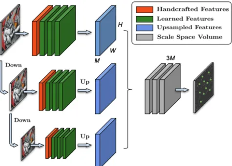
features at different scale levels. feature maps are upsampled and concate-nated.Last learned filter combines the Scale Space Volume to obtain the final response map[4] . . . 18 3.2 The graph neural network transforms the coordinates into features of the

points, so that a simple inference algorithm can successfully do feature matching[4] . . . 19 3.3 Block Diagram of iris feature extraction to microsaccades detection [4] . . . 20 3.4 TensorBoard graph visualization of a convolutional neural network model[5] 22 4.1 DoG pyramid used for SIFT . . . 26 4.2 Neighborhood for the initial scale-space extrema detection . . . 27 4.3 Training steps for the image I and I0[6] . . . 30

4.4 Schematic representation of our training method of Glampoint algorithm. . 30 4.5 LIFT feature extraction pipeline.The pipeline consists of three components:

the Detector, the Orientation Estimator, and the Descriptor.[7] They are tied together with differentiable operators to preserve end-to-end differentiability 31

(10)

LIST OF FIGURES 9

4.6 LIFT algorithm is trained on Siamese Neural network[7].Siamese training architecture with four branches, which takes as input a quadruplet of patches: PatchesP1 andP2(blue) correspond to different views of the same physical

point, and are used as positive examples to train the Descriptor;P3 (green)

shows a different 3D point, which serves as a negative example for the Descriptor; andP4 (red) contains no distinctive feature points and is only

used as a negative example to train the Detector. Given a patch P, the Detector, the softargmax, and the Spatial Transformer layer Crop provide all together a smaller patch p inside P. p is then fed to the Orientation Estimator, which along with the Spatial Transformer layer Rot, provides the rotated patchpθ that is processed by the Descriptor to obtain the final description

vector d. . . 32

4.7 The SuperGlue architecture: SuperGlue is made up of two major components: the attentional graph neural network, and the optimal matching layer. The first component uses a keypoint encoder to map keypoint positions p and their visual descriptors d into a single vector, and then uses alternating self- and cross-attention layers (repeated L times) to create more powerful representations f. The optimal matching layer creates an M by N score matrix, augments it with dustbins, then finds the optimal partial assignment using the Sinkhorn algorithm (for T iterations)[8] . . . 34

5.1 SIFT Matching frame by frame. . . 37

5.2 LIFT Output using the transfer Learning. . . 38

5.3 Glampoints outfut frame by frame. . . 39

5.4 SIFT in Glampoint network outfput frame by frame. . . 39

5.5 SuperGlue outfput frame 0and frame10. . . 40

5.6 SuperGlue outfput frame 0and frame100.. . . 40

5.7 SuperGlue outfput frame 0and frame1. . . 41

(11)

Chapter 1

Introduction

1.1 Overview

The iris feature detection is an important part of eye tracking as well as to identify many macula generated deceases in medical sciences. Thus we studied the survey of the texture analysis [9]to identify the seven practiced approaches for iris detection. The survey had seven classes: statistical approaches, structural approaches, transform-based approaches, model-based approaches, graph-based approaches, learning-based approaches, and entropy-based approaches which so far been used for the feature extraction in medical images. Among these seven classes four categories are classified as statistical approaches, structural approaches, transform-based approaches, and model-based approaches are recently well used for feature extraction.Though all the classes have their significant advantages along with some improvement areas or limitations, we chose to compare the deep learning based approaches as this is dealing with convolution neural networks that helps us to build and predict the models better than any hand crafted features or algorithms. There is also a lot of new methods to explore in deep learning as it has supervised learning, semi-supervised and reinforcement learning. This research also found the cross-entropy based approaches compelling as there is not much reference with the iris dataset or any other medical images.

(12)

CHAPTER 1. INTRODUCTION 11

1.2 Motivation

The study is based on the identification of the monocular microsaccades. The small rapid eye movements that occur in only one eye at a time, is not very easy to detect. Our research started with the video-based eye trackers which showed that microsaccades have very sensitive and fast feature action in the iris, [1] to detect smoothly. So we extended our research to the iris feature detection part and not only on microsaccades[1]. We mostly studied the recent published papers to replicate current knowledge base with our existing iris dataset [10]. We also wanted to maximize the feature extraction process to the existing algorithms to make our research more robust.

(13)

Chapter 2

Data Collection

Figure 2.1 consists of sample images from our experiment. The size of the circles connecting the scanpaths depicts the amount of time a subject fixated in that particular location.

2.1 Subject

The eye movements was recorded for( σ= 12) with normal or corrected-to-normal (two out

of seven subjects) vision. Observers with a varying range of iris pigmentation were selected for the experiment. The experiment was conducted with the approval of the Institutional Review Board, and all participants provided informed consent before starting the experiment by the MVRL lab members[3].

2.2 Experiments Performed

Every observer performed a sequence of tasks. Initially, 12 calibration targets were displayed on the screen in a pseudo-random pattern to allow the maximum number of changes in horizontal and vertical directions, as shown in Figure2.2. Each target consisted of concentric circles, the larger of which initially subtended an angle of 1.0 degrees. The target first grew to a size of 1.34 degrees then decreased to a size of 0.5 degrees before disappearing after one second, as shown in Figure??. The field of view of the calibration targets was14.19◦X9.68◦.

The calibration was followed by the tasks described in the following section. [3].

(14)

CHAPTER 2. DATA COLLECTION 13

Figure 2.1: Grayscale version of the image captured with the setup(Top row).Bottom row contains cropped version of left eye for different subjects with corrected glasses[3]

2.2.1 Task 01: Calibration Verification Task

Six calibration verification targets were shown in sequence, subtending a total angle of

10.02◦X3.99◦. The delay between the disappearance of one target and the appearance of

the next target was on average 31 ms (σ = 5). The calibration verification points were

(15)

Figure 2.2: Calibration targets designed to maximize variations in gaze angle and directions[3]

Figure 2.3: Visualization of target size animation over 1-second interval: each frame was displayed for 1/30 second[3].

MVRL lab members evaluated the accuracy and precision with which the methods predicted gaze on the verification targets, assuming that the observer fixated each target. Accuracy measures were based on the difference between the displayed target position and the mean reported gaze position of the stable fixation window. The fixation window was determined from a rolling 450 ms window with a minimum dispersion search after the target was displayed on the screen.

Another essential metric was precision during fixations. Sample-to-sample root mean square error (S2S-RMS) and standard deviation (STD) are two widely used metrics to measure the precision of eye-trackers. S2S-RMS is calculated on temporally adjacent data points, its value relays information about the spatio-temporal aspects of a system that are absent from STD

(16)

measures. S2S-RMS is also inherently sensitive to the update rate of the eye-tracker[3].

2.2.2 Task 02: Smooth Pursuit Task

To evaluate the eye-tracking methodology, we evaluated two tasks that require very high precision: microsaccade detection and smooth pursuit. For a smooth-pursuit task, observers followed a moving target on a ramp (linear-trajectory) at different velocities (mean=4.6 deg/s, σ= 1.9) with 17 random directional changes.

Measurement of accuracy and precision in a smoothpursuit task is not straightforward. proposed a method to determine the accuracy based on how closely the smooth-pursuit signal matches the target stimulus. A quantitative smooth pursuit score based onthe position and velocity was reported based on the Euclidean distance and differences in speed at every timestamp with respect to the smooth-pursuit target stimulus.

We propose a method for measuring precision during smooth pursuit using S2S-RMS and STD after ‘detrending’ the raw data. ’Detrending’ a signal subtracts the best-fit line/curve from the data [Moncrieff et al. 2004]. So, a constant velocity term can be removed from the smooth-pursuit data resulting in nearly zerovelocity signal. In any smooth pursuit movement with randomly changing directions, it is observed that there is a latency of 100130 ms after the direction change. At that point, the eye either begins moving at approximately the correct velocity (but is lagging the target due to the latency), or the movement starts with a small saccade in the direction of the stimulus. In either case, the eye velocity is then typically similar to that of the target but lags in position. Finally, any positional offset between the eye and target is corrected by a second ‘catch-up’ saccade, as shown in Figure 8. At that point, the eye position and velocity match the stimulus.

In our proposed smooth-pursuit precision metric, we initially find the time interval where both the eye position and eye velocity are closest to the stimulus position and velocity. The eye position at this moment is referred to as the starting point. Similarly, we compute the ending point just before the stimulus changes direction. An equation describing the line joining the starting and ending gaze points is computed. The gaze signal is detrended using this signal (line), resulting in a signal with zero mean velocity and can be analyzed in the same way as a fixation signal. We can thus compute the precision (S2S-RMS and STD) for the detrended signal.

2.2.3 Task 03: Microsaccade Detection Task

Motivated by [Shelchkova et al. 2018] and [Chaudhary and Pelz 2019], we evoked small, voluntary eye movements with a Snellen acuity chart by displaying a sequence of fixation

(17)

targets on the teleprompter screen. Any voluntary or involuntary saccade less than 0.5 ◦ is considered as microsaccade in this paper following [Chaudhary and Pelz 2019; Engbert and Kliegl 2003; Otero-Millan et al. 2008; Shelchkova et al. 2018; Troncoso et al. 2008]. There were two elements in this task; first, the observer was asked to fixate on a series of thin color bars (6 bars, each (5.2x12 arcmin)), then on six colored boxes, alternating in size between 12x12 and 5.2x12 arcmin. Each target was displaced from the previous target in the horizontal direction by 0.2 degrees (12 arcmin). The total expected number of small eye movements was ten (five each for the color bars and boxes).

The number of microsaccades detected when the observer looked to the different color bars/boxes. Horizontal eye movements detected within 100 - 500 ms of each target onset were identified as microsaccades. Note that horizontal cyclopean velocity was used for microsaccade identification. We used the method described in [Chaudhary and Pelz 2019], where the velocity signal is filtered with a 1D total variational denoising filter (regularization value of 0.05). After denoising the velocity signal, a threshold value is determined with an adaptive algorithm by fitting two velocity distributions representing noise and microsaccade based on Gaussian mixture models. Velocities above the adaptive threshold are identified as microsaccades based on the VelocityThreshold Identification algorithm (I-VT) [Salvucci and Goldberg 2000]. We refer the reader to [Chaudhary and Pelz 2019] (Section: Microsaccade detection) for additional details.

(18)

Chapter 3

Literature Review

3.1 Glampoints:Greedily Learned Accurate Match points

-Review

Deep learning algorithms that we discussed in this chapter are mostly derived using the synthetic images, but the GLAMpoints [6]used both synthetic and preprocessed dataset along with and some natural datasets. GlAMpoints [6] the network used the handcrafted feature detectors like SIFT, LIFT, ORB. We learned these detectors to work along with the CNN architectures that were shown to outperform state-of-the-art computer vision detectors. Learned Invariant Feature Transform (LIFT) uses patches to train a fully differentiable deep CNN for interest point detection, orientation estimation, and descriptor computation based on supervision from classical Structure from Motion (SfM) systems. SuperPoint: Self-Supervised Interest Point Detection and Description [? ? ] introduced a self-supervised

framework for training interest point detectors and descriptors. It rises to state-of-the-art homography estimation results on HPatches when compared to SIFT , LIFT, and Oriented Fast and Rotated Brief (ORB).And then compared the network performance with different handcrafted features. After the comparison, the paper stated that the GLAMpoint algorithm gives the best results compared to the rest of the combinations.

Thus we decided to study more on deep learning approaches and how the the CNN-based feature detector the GLAMpoints: Greedily Learned Accurate Matchpoints[6] is designed as a semi-supervised learned method for keypoint detection. In general, features are often optimized for repeatability (such as LF-NET) and not for the quality of the associated matches between image pairs. The training procedure used a reward concept that is unique

(19)

CHAPTER 3. LITERATURE REVIEW 18

and is related to the Reinforcement Learning(RL) to extract repeatable, stable interest points with a uniform coverage specifically designed to maximize correct matching on a specific domain which is here the funds retinal images. The challenge is shown on retinal slit-lamp images.[6]and paper also suggested that the method is also giving excellent results on the natural images. So later in the method section we described the method step by step.

Figure 3.1: Key.Net architecture combines handcrafted and learned filters to extract features at different scale levels. feature maps are upsampled and concatenated.Last learned filter combines the Scale Space Volume to obtain the final response map[4]

3.2 Key.Net: Keypoint Detection by Handcrafted and Learned

CNN Filters.

On the other hand, we also studied the key point detection[4] 2019 IEEE published paper, where the ground truth was need and there was a separated layer where the hand crafted features where identified. So this algorithm also used the convolution neural network, but

(20)

with an extra layer where the hand crafted features are identified and the ground truth is been set.

“Key.Net: Keypoint Detection by Handcrafted and Learned CNN Filters.”[4] The shallow multiscale architecture was used for the keypoint detection task that combines handcrafted and learned CNN filters. Here the author structured the learned filters by using different handcrafted filters to localize, score and rank the repeatable features. And the scale-space representation is used within the network to extract key points at different levels. The paper proposed a new design of a loss function to detect robust features that exist across a range of scales and to maximize the repeatability score. But GLAMpointsGLAMpoints[6] out performed this key point detection process in the literature, which we have to replicate with our own dataset and validate the results. Figure3.2 shows a schematic representation of our second approach in extending Keypoint Detection by Handcrafted and Learned CNN algorithm and is a flowchart representing the methodology behind our analysis.

Figure 3.2: The graph neural network transforms the coordinates into features of the points, so that a simple inference algorithm can successfully do feature matching[4]

(21)

Figure 3.3: Block Diagram of iris feature extraction to microsaccades detection [4]

3.3 Deep Graphical Feature Learning for the Feature

Match-ing Problem.

In this paper[4], we studied a graph neural network that can transform weak local geometric features into rich local features for the geometric feature matching problem. As opposed to the Traditional approaches, use pairwise or higher-order handcrafted geometric features to get robust matching, and this requires solving NP-hard assignment problems. This method is also trained with synthetic data and is then applied to both synthetic and real-world feature matching problems with feature deformations caused by noise, rotation, and outliers. This proposed method showed a great result on both synthetic and real datasets demonstrated the effectiveness of the proposed method. The results suggest that with quite limited local information, the graph neural network is still able to get rich local representations through message passing between nodes.

3.4 Motion tracking of iris features to detect small eye

move-ments

From this paper [4] we have gathered the fundamental idea of the iris features and how the eye movements are monitored by extracting the motion vectors of multiple iris features. This requires a high frame-rate, high-resolution camera to capture a video of an observer’s face containing the eyes and surrounding regions. We studied multiple papers to understand the concepts of the article as to how a trained convolutional network (CNN) (LeCun et al., 1998) is used to segment the iris from each frame to extract features only from the region of interest. Then Speeded Up Robust Features (SURF) feature descriptors (Bay et al., 2006) are used to extract feature vectors which is designed to ensure high quality motion

(22)

signals which are then matched in consecutive frames using brute force matching followed by random sample consensus (RANSAC)and homography. The author performed the tracking through the geometric median of these matched keypoints excludes outliers, and the velocity is approximated by scaling the sampling rate [2]. Microsaccades are then identified by thresholding the velocity estimate. For the end to end video-based eye-tracker, the head motion compensation is done across each frame; a hybrid cascaded similarity transformation model is introduced using tracking and matching of features of rectangular patches in regions of the observer’s cheek. This idea made our study more robust and decided to focus on replacing the handcrafted features for feature detection that eventually will improve the performance of the eye-tracker.Figure3.3 shows a schematic representation of our approach in extracting the iris features and is a flowchart representing the methodology behind the paper implementation.

3.5 TensorFlow: Large-Scale Machine Learning on

Heteroge-neous Distributed Systems

The last paper [5] that we have chosen to discuss is “TensorFlow: Large-Scale Machine Learning on Heterogeneous Distributed Systems.”TensorFlow is an open-source, flexible data flow based programming model, as well as a single machine and distributed implementations of this programming model. The system is borne from real-world experience in conducting research and deploying more than one hundred machine learning projects throughout a wide range of Google products and services. This is an open-sourced version of TensorFlow, and they hoped that a vibrant shared community (like us)develops around the use of TensorFlow as it has a defined and structured model.

Deep learning concepts are defined and implemented in the tensor flow and the most significant benefit for a researcher is that we have the tensor board where we can see and understand the step by step algorithm, data processing efficiency or the area where we need to tweak the algorithm or rewrite the method or may be the image needs to be pre-processed. And the performance results also can be generated as of the automated graphs that show the detection performance of the given prediction model. So we have figured that this paper is a good paper to review.

3.6 Reviewed paper:Advantages and Disadvantages

Typically, feature extraction and matching of two images comprise four steps: detection of interest points, computing feature descriptor for each of them, matching of corresponding

(23)

Figure 3.4: TensorBoard graph visualization of a convolutional neural network model[5]

key points, and estimation of a transformation between the images using the matches. So we can conclude that the detection step influences every further step and crucial for a successful registration. It requires high image coverage and stable key points in low contrast images, which is implemented with the GLAMpoint detectors that extract repeatable, stable interest points with a dense coverage. The GLAMpoint paper not only defined the new process but also showed a comparison with other well known handcrafted feature detectors.

The challenge lies in the training procedure as this is complicated, and by their self-supervision, the network can only find corner points. Local Feature Network (LF-NET) is the closest to the proposed GLAMpoints method: a keypoint detector and descriptor is trained end-to-end in a two-branch set-up, one being differentiable and feeding on the output of the other non-differentiable branch. However, they optimized their detector for repeatability between image pairs, not taking into account the matching performance. This can lead to false maching points or increases the failure rate.

The main learning point from the Keypoint paper is that by using handcrafted filters, we can significantly reduce the complexity of the architecture leading to a detector with 280 learnable parameters and inference of175frames per second.And then proposed detectors

(24)

lead to state-of-the-art matching performance when used with a descriptor on viewpoint. Entropy-based measures have been proposed since the 2000’s, to process time series (unidi-mensional data) and shown fascinating results in domains as the biomedical field. Many papers have been published on the use of these entropy measures before 2011, and we could find also some before 2016. But they were all restricted to the processing of time series and no extension to images were suggested. As the entropy-based approaches developed based on time series, we can replicate the method to detect the iris feature patterns (this can be an exciting find for a researcher) . On the contrary unidimensional cases in the information-theory field, have shown exciting results. So similar algorithms can be used or studied for iris feature extraction in the biomedical field. There are two-dimensional sample entropy, two-dimensional distribution entropy, and two-dimensional multiscale entropy. As a reference, we studied these new texture features VOLUME 7, 2019 A. Humeau-Heurtier: Texture Feature Extraction Methods: A Survey extraction methods are simple to implement, based on substantial theoretical aspects because they are extensions of already well-known 1D measures, and found the results very compelling.

As our focus area is on the iris images that require invariant features for rotation,translation, scaling based applications, the number of possible methods decreased significantly. One of the limitations that we have observed is that this paper did not discuss particular cases instead gave a broad general idea of the methods. But the two most recent classes are the learning-based approaches, and the entropy-based approaches are very useful for our iris feature extraction from the iris images. So in the method chapter, we choose to discuss and implement the algorithms with significant good results.

(25)

Chapter 4

Methods and Implementation

4.1 The Summary Statistics Method

The summary statistics (SS) from [1] method acts as a baseline for our method of analysis. The input to this method is the mean number of fixations and fixation duration. Considering a trial with T fixations, we can mathematically represent its information as;

4.2 Handcrafted Method

4.2.1 SIFT:Scale Invariant Feature Transform

Scale Invariant Feature transform [11] is a handcrafted method feature detection method. Here a high level road map is described without dwelling on the math. SIFT identifies keypoints that are distinctive across an image’s width, height, and most importantly, scale. By considering scale, we can identify keypoints that will remain stable (to an extent) even when the template of interest changes size, when the image quality becomes better or worse, or when the template undergoes changes in viewpoint or aspect ratio. Moreover, each keypoint has an associated orientation that makes SIFT features invariant to template rotations. Finally, SIFT will generate a descriptor for each keypoint, a 128-length vector that allows keypoints to be compared. These descriptors are nothing more than a histogram of gradients computed within the keypoint’s neighborhood. Most of the tricky details in SIFT relate to scale space, like applying the correct amount of blur to the input image, or converting keypoints from one scale to another. In 2004, D.Lowe, University of British Columbia, came up with this new algorithm, Scale Invariant Feature Transform (SIFT) in his

(26)

CHAPTER 4. METHODS AND IMPLEMENTATION 25

paper, Distinctive Image Features from Scale-Invariant Keypoints, which extract keypoints and compute its descriptors. There are mainly four steps involved in SIFT algorithm. We will see them one-by-one. Ref: https://lerner98.medium.com/implementing-sift-in-python-36c619df7945 There are mainly four steps involved in SIFT algorithm. We will see them one-by-one.

Scale-space Extrema Detection

From the image above, it is obvious that we can’t use the same window to detect keypoints with different scale. It is OK with small corner. But to detect larger corners we need larger windows. For this, scale-space filtering is used. In it, Laplacian of Gaussian is found for the image with various σ values. LoG acts as a blob detector which detects blobs in various

sizes due to change in . In short,σ acts as a scaling parameter. For eg, in the above image,

gaussian kernel with low gives high value for small corner while gaussian kernel with high fits well for larger corner. So, we can find the local maxima across the scale and space which gives us a list of (x,y,) values which means there is a potential keypoint at (x,y) at scale. But this LoG is a little costly, so SIFT algorithm uses Difference of Gaussians which is an approximation of LoG. Difference of Gaussian is obtained as the difference of Gaussian blurring of an image with two different , let it be and k. This process is done for different octaves of the image in Gaussian Pyramid. It is represented in below image:

Once this DoG are found, images are searched for local extrema over scale and space. For eg, one pixel in an image is compared with its 8 neighbours as well as 9 pixels in next scale and 9 pixels in previous scales. If it is a local extrema, it is a potential keypoint. It basically means that keypoint is best represented in that scale. It is shown in below image:

Regarding different parameters, the paper gives some empirical data which can be summa-rized as, number of octaves =4, number of scale levels =5, initialσ =1.6, k=−√2 etc as

optimal values.

Keypoint Localization

Once potential keypoints locations are found, they have to be refined to get more accurate results. They used Taylor series expansion of scale space to get more accurate location of extrema, and if the intensity at this extrema is less than a threshold value (0.03 as per

the paper), it is rejected. This threshold is called contrastThreshold in OpenCV DoG has higher response for edges, so edges also need to be removed. For this, a concept similar to Harris corner detector is used. They used a 2x2 Hessian matrix (H) to compute the

(27)

Figure 4.1: DoG pyramid used for SIFT

larger than the other. So here they used a simple function, If this ratio is greater than a threshold, called edgeThreshold in OpenCV, that keypoint is discarded. It is given as10 in

paper. So it eliminates any low-contrast keypoints and edge keypoints and what remains is strong interest points.

Orientation Assignment

Now an orientation is assigned to each keypoint to achieve invariance to image rotation. A neighbourhood is taken around the keypoint location depending on the scale, and the gradient magnitude and direction is calculated in that region. An orientation histogram with 36 bins covering 360 degrees is created (It is weighted by gradient magnitude and

gaussian-weighted circular window with equal to 1.5 times the scale of keypoint). The

highest peak in the histogram is taken and any peak above 80 percent of it is also considered to calculate the orientation. It creates keypoints with same location and scale, but different directions. It contribute to stability of matching.

(28)

Figure 4.2: Neighborhood for the initial scale-space extrema detection

Keypoint Descriptor

Now keypoint descriptor is created. A 16x16 neighbourhood around the keypoint is taken. It is divided into 16 sub-blocks of 4x4 size. For each sub-block, 8 bin orientation histogram is created. So a total of 128 bin values are available. It is represented as a vector to form keypoint descriptor. In addition to this, several measures are taken to achieve robustness against illumination changes, rotation etc.

Keypoint Matching

Keypoints between two images are matched by identifying their nearest neighbours. But in some cases, the second closest-match may be very near to the first. It may happen due to noise or some other reasons. In that case, ratio of closest-distance to second-closest distance is taken. If it is greater than 0.8, they are rejected. It eliminates around90%of

(29)

a summary of SIFT algorithm. For more details and understanding, reading the original paper is highly recommended. We need to remember one thing, this algorithm is patented. So, this algorithm is included in the opencv contrib repo.

4.3 Deep Learning Method

In machine learning, most classifiers require all input feature vectors to have a fixed-dimensionality. However, the number of fixations obtained from each trial varies. The reason behind turning a trial’s fixation features into Fisher Vectors is to overcome this challenge and to enable MFPA algorithms to capture diagnostic information.

4.3.1 Glampoints: Greedily Learned Accurate Match points

Greedily Learned Accurate Match Points is a novel CNN-based feature point detector learned in a semi-supervised manner[6]. This algorithm extracts repeatable, stable interest points with a dense coverage, specifically designed to maximize the correct matching in a specific domain, which is in contrast to conventional techniques that optimize indirect metrics. Classical detectors yield unsatisfactory results due to low image quality and insufficient amount of low-level features, but this detector showed significantly better than the classical detectors as well as state-of-the-art CNN-based methods are used for matching and registration for retinal images. Feature extraction and matching of two images comprise mainly four steps: detection of interest points, computing feature descriptor for each of them, matching of corresponding keypoints and estimation of a transformation between the images using the matches. To implement the algorithm we followed the following tasks to define our implementation work flow. Let B be the set of base images of sizeH×W.

At every step i, an image pair Ii,Ii0 is generated from an original image Bi by applying

two separate, randomly sampled homography transforms gi ,gi0 . Images Ii and Ii0 are

thus related according to the homography HIi ,Ii0 = gi0gi¬1 . On top of the geometric

transformations, standard data augmentation methods are used: gaussian noise, changes of contrast, illumination, gamma, motion blur and the inverse of image. A subset of these appearance transformations is randomly chosen for each image I andI0.

Training

We define our learned function fθ(I) → S, where S denotes the pixel-wise feature point

probability map of size H×W. Lacking a direct ground truth of keypoint locations, a

delayed reward can be computed instead. We base this reward on the matching success, computed after registration[6]. The training proceeds as follows:

(30)

1. Given a pair of images I ∈ _RH×W_and _I0 _∈

RH×Wrelated with the ground truth

homographyH =H I,I0 , our model provides a score map for each image,S =fθ(I)

andS0 =fθ(I0)

2. The locations of interest points are extracted on both score maps using standard non-differentiable NonMax-Supression (NMS), with a window size w.

3. A 128 root-SIFT, feature descriptor is computed for each detected keypoint.

4. The keypoints from image I are matched to those of imageI0 and vice versa using a

brute force matcher. Only the matches that are found in both directions are kept. 5. The matches are checked according to the ground truth homography H. A match is

defined as true positive if the corresponding keypoint x in image I falls into and

-neighborhood of the pointx0inI0after applying H. This is formulated askH∗(x−x0)k≤

, where we choseas 3 px.

Let T denote the set of true matches. If a given feature point ends up in the set of true positive points, it gets a positive reward. All other points/pixels are given a reward of

θ. Consequently, the reward matrixR∈RH×W for a keypoint (x, y) can be defined

as follows:

Rx, y= (

1, f or(x, y)∈T

0, otherwise (4.1)

This leads to the following loss function:

Lsimple(Θ, I) =X(f θ(I)−R)2 (4.2)

Given a reward R with mostly zero values, thefΘ converges to a zero output. Hard mining

has been shown to boost training of descriptors[6].

Figure4.5 shows a schematic representation of our second approach in extending Glampoint algorithm and Figure4.3 is a flowchart representing the methodology behind our analysis.

Evaluation Criteria

(31)

Figure 4.3: Training steps for the image I andI0[6]

Figure 4.4: Schematic representation of our training method of Glampoint algorithm.

1. Repeatability: this criterion described the percentage of detected points x ∈ P

in image I that are within an −distance( = 3) to points x0 ∈ P0 in I0 after

transformation with HI,I0 :

k{x∈P, x0 ∈P0kkk|HI,I0∗(x−x0)k|< }k

kPk+kP0k (4.3)

2. Matching Performance: Matches were found using the Nearest Neighbor Distance

Ratio (NNDR) strategy, as proposed in [6]: two keypoints are matched if the descriptor distance ratio between the first and the second nearest neighbor is below a certain threshold t. Then, the following metrics were evaluated

(32)

(a)AUC, area under the ROC curve created by varying the value of t.

(b)M.score, the ratio of correct matches over the total number of keypoints extracted

by the detector in the shared viewpoint region.

(c)Coverage fraction, measures the coverage of an image by correctly matched key

points. A coverage mask was generated from correctly matched key points, each one adding a disk of fixed radius(25px)

4.3.2 LIFT: Learned Invariant Feature Transform

Authors from [7] We introduce a novel Deep Network architecture that implements the full feature point handling pipeline, that is, detection, orientation estimation, and feature description. While previous works have successfully tackled each one of these problems individually, we show how to learn to do all three in a unified manner while preserving end-to-end differentiability. We then demonstrate that our Deep pipeline outperforms state-of-the-art methods on a number of benchmark datasets, without the need of retraining.

Figure 4.5: LIFT feature extraction pipeline.The pipeline consists of three components: the Detector, the Orientation Estimator, and the Descriptor.[7] They are tied together with differentiable operators to preserve end-to-end differentiability

Problem formulation and Training procedure

This paper[7] first formulate the entire feature detection and description pipeline in terms of the Siamese architecture depicted by Figure??. And then we discuss discuss the type

of data we need to train our networks and how to the data is collected. Afterwards the training steps are explained step by step. This is the algorithm were we did not use SIFT (Scale Invariant Feature Transform) at all.

(33)

Figure 4.6: LIFT algorithm is trained on Siamese Neural network[7].Siamese training architecture with four branches, which takes as input a quadruplet of patches: Patches

P1 and P2(blue) correspond to different views of the same physical point, and are used

as positive examples to train the Descriptor;P3 (green) shows a different 3D point, which

serves as a negative example for the Descriptor; andP4 (red) contains no distinctive feature

points and is only used as a negative example to train the Detector. Given a patch P, the Detector, the softargmax, and the Spatial Transformer layer Crop provide all together a smaller patch p inside P. p is then fed to the Orientation Estimator, which along with the Spatial Transformer layer Rot, provides the rotated patchpθ that is processed by the

Descriptor to obtain the final description vector d.

The algorithm uses image patches as input, rather than full images. This makes the learning scalable without loss of information, as most image regions do not contain keypoints. The patches are extracted from the keypoints used by a SfM pipeline. We take them to be small enough that we can assume they contain only one dominant local feature at the given scale, which reduces the learning process to finding the most distinctive point in the patch. To train our network we create the four-branch Siamese architecture pictured in Figure 4.6. Each branch contains three distinct CNNs, a Detector, an Orientation Estimator, and a Descriptor. For training purposes, we use quadruplets of image patches. Each one includes two image patchesP1 andP2 , that correspond to different views of the same 3D point, one

image patch P3 , that contains the projection of a different 3D point, and one image patch P4 that does not contain any distinctive feature point. During training, the i-th patchPi of

each quadruplet will go through the i-th branch.

To achieve end-to-end differentiability, the components of each branch are connected as follows[7]:

(34)

1. Given an input image patch P, the Detector provides a score map S.

2. We perform a soft-argmax on the score map S and return the location x of a single potential feature point.

3. We extract a smaller patch p centered on x with the Spatial Transformer layer Crop Figure 4.6. This serves as the input to the Orientation Estimator.

4. The Orientation Estimator predicts a patch orientationθ.

5. We rotate p according to this orientation using a second Spatial Transformer layer, labeled as Rot in Figure4.6, to producepθ.

6. pθ is fed to the Descriptor network, which computes a feature vector d.

Spatial Transformer layers are used only to manipulate the image patches while preserving differentiability. They are not learned modules[7]. Also, both the location x proposed by the Detector and the orientation θfor the patch proposal are treated implicitly, meaning

that we let the entire network discover distinctive locations and stable orientations while learning.

Limitations of the algorithm

This network consists of components with different purposes, learning the weights is non-trivial. The early attempts at training the network as a whole from scratch were unsuccessful. Therefore the network is designed as a problem-specific learning approach that involves learning first the Descriptor, then the Orientation Estimator given the learned descriptor, and finally the Detector, conditioned on the other two. This allows to tune the Orientation Estimator for the Descriptor, and the Detector for the other two components[7].

(35)

4.3.3 SuperGlue: Learning Feature Matching with Graph Neural net-works

This algorithm is published in CVPR2020conference [8] and the paper introduces SuperGlue,

a neural network that matches two sets of local features by jointly finding correspondences and rejecting non-matchable points. Assignments are estimated by solving a differentiable optimal transport problem, whose costs are predicted by a graph neural network.

SuperGlue outperforms other learned approaches and achieves state-of-the-art results on the task of pose estimation in challenging real-world indoor and outdoor environ-ments. The proposed method performs matching in real-time on a modern GPU and can be readily integrated into modern Structure for motion or Simaltenious Localization and Mapping(SLAM) systems. The code and trained weights are publicly available at github.com/magicleap/SuperGluePretrainedNetwork.

Figure 4.7: The SuperGlue architecture: SuperGlue is made up of two major components: the attentional graph neural network, and the optimal matching layer. The first component uses a keypoint encoder to map keypoint positions p and their visual descriptors d into a single vector, and then uses alternating self- and cross-attention layers (repeated L times) to create more powerful representations f. The optimal matching layer creates an M by N score matrix, augments it with dustbins, then finds the optimal partial assignment using the Sinkhorn algorithm (for T iterations)[8]

The SuperGlue Architecture

In the image matching problem[8], some regularities of the world could be leveraged: the 3D world is largely smooth and sometimes planar, all correspondences for a given image pair derive from a single epipolar transform if the scene is static, and some poses are more likely than others. An effective model for feature matching should aim at finding all

(36)

correspondences between reprojections of the same 3D points and identifying keypoints that have no matches. SuperGlue is formulated Figure 4.7 as solving an optimization problem, whose cost is predicted by a deep neural network. This alleviates the need for domain expertise and heuristics – the network learn relevant priors directly from the data.

Problem Formulation:[8], Consider two images A and B, each with a set of keypoint

positions p and associated visual descriptors d – we refer to them jointly (p, d) as the local features. Positions consist of x and y image coordinates as well as a detection confidence c,

pi :=(x, y, c)i. Visual descriptorsdi∈RD can be those extracted by a CNN like Superpoint

or traditional descriptor like SIFT. Images A and B have M and N local features, indexed

A:={1, ..., M} and B:={1, ..., N}, respectively.

Partial Assignment:[8] Constraints i) a keypoint can have at most a single correspondence

in the other image; and ii)some keypoints will be unmatched due to occlusion and failure of the detector that correspondences derive from a partial assignment between the two sets of keypoints. For the integration into downstream tasks and better interpretability, each possible correspondence should have a confidence value. We consequently define a partial soft assignment matrix P∈[0,1]M×N as :

P1N ≤1M.andPT1M ≤1N

The goal is to design a neural network that predicts the assignment P from two sets of local features.

And this paper[8] demonstrates the power of attention-based graph neural networks for local feature matching. SuperGlue’s architecture Figure 4.7 uses two kinds of attention: (i) self-attention, which boosts the receptive field of local descriptors, and (ii) cross-self-attention, which enables cross-image communication and is inspired by the way humans look back-and-forth when matching images. This method elegantly handles partial assignments and occluded points by solving an optimal transport problem. In the CVPR-2020 conference, SuperGlue

achieved significant improvement over existing approaches, enabling highly accurate relative pose estimation on extreme wide-baseline indoor and outdoor image pairs. In addition, SuperGlue runs in real-time and works well with both classical and learned features. In conclusion, this learnable middle-end replaces handcrafted heuristics with a powerful neural model that simultaneously performs context aggregation, matching, and filtering in a

(37)

(38)

Chapter 5

Results

Figure 5.1: SIFT Matching frame by frame.

As we run the four feature extraction algorithms, we clearly could observe that SuperGlue[8] out performed the rest of the algorithms in terms of the feature matching. We also can see the prominent result for Glampoints [6]. While we are very optimistic about the LIFT [7], we could not train or run the algorithm due to the package support. LIFT[7] is built in Theano and Caffee which is not supported with current python packages. Thus we run the transfer learning on the pre-trained model and vividly the algorithm was not better than the other two algorithms and we could not clearly understand how the segmentation is been done in the algorithm.

Figures 5.1 represent the first two frame matches in the RIT-Eyes dataset [10] where we can

(39)

CHAPTER 5. RESULTS 38

see clear feature points and the number of matches in the two consecutive frames.

Figures 5.3,represent the Glampoint [6] consecutive two frame iris feature extraction, along with the homography, and the RANSAC Image where all the correct region is been se-lected

Figures 5.4,represent the Glampoint [6] consecutive two frame iris feature extraction, along with the homography, and the RANSAC Image where all the correct region is been selected.

Figure 5.2: LIFT Output using the transfer Learning.

Figures 5.2, represent the LIFT[7] consecutive two frame output with boundary regions. Here we did not generate the matching as from the images we can see that there is less feature points on the iris and after the transfer learning the image frame was also reduced. Thus we choose to keep the result for our reference, but not to use for the future work

Figures 5.5, SuperGlue[8] algorithm did extract feature points and matched simultaneously and the results are clearly better than SIFT and Glampoints.Here we compaired the first and the 10th frame to compare the matches. We could see that even after the shift in the frames, SuperGlue matches significantly better than out other two algorims and our target algorithm SIFT can be replaced with SuperGlue.

Figures 5.6, SuperGlue[8] represent a geat deal of matching points and this scenario is prevelant in all other consecutive frames.

(40)

Figure 5.3: Glampoints outfut frame by frame.

Figure 5.4: SIFT in Glampoint network outfput frame by frame.

consecutive two frames in the given dataset.

Figures 5.8, [8] algorithm did extract feature points and matched simultaneously, but here in these two consecutive frames there are some errors or mismatch, we can observe. This is

(41)

also shows the effectiveness of the algorithm as it generates less than.0001%errors. And

we can consider here that the algorithm considers the outliers as well

Figure 5.5: SuperGlue outfput frame 0 and frame10.

(42)

Figure 5.7: SuperGlue outfput frame 0 and frame1.

h]

(43)

Chapter 6

Summary

6.1 Conclusions

This research paper review clearly showed a good deal of opportunities to explore the current deep learning approaches using versatile iris dataset and exploit and tweak the handcrafted methods with the convolution neural networks (CNN) to get the best and robust feature detectors to create a state-of-the-art eye-tracking device. The target of my review paper was to read and understand the available feature detectors. So, in this regard, I have studied the survey paper and then moved to the CNN-based feature detectors as GLAMpoints and the key point detectors. From there, I changed my research read to the Tensorflow as we have understood that the need for understanding the network is crucial. There are significant variations in the existing systems which are designed with both the combinations of handcrafted and CNN based approaches. As our initial interest was on the detection of the microsaccades, we studied the Motion tracking of iris features to detect small eye movements paper [4]and also read the “An effective and fast iris recognition system based on a combined multiscale feature extraction technique”(2007).Few other articles we cited and studies to understand the mathematical models to implement as well as replicate (possible to do/ justify the knowledge base).

(44)

CHAPTER 6. SUMMARY 43

6.2 Applications and Future Work

The first part of the research was to detect the iris feature points from the video images, which we successfully tracked and matched using the deep neural network(instead of handcrafted methods). Now my main goal is to generate the distribution models using these feature points frame by frame and use these distribution parameters as priors in the Bayesian Neural Network to generate my future prediction models or the posterior distributions. So I can calculate the velocity and speed of the microsaccades in the eye(Small rapid eye movements)in the paper [1]. This is quite a challenging task and we know the significance of the future task.

(45)

Bibliography

[1] Aayush K. Chaudhary and Jeff B. Pelz. Motion tracking of iris features to detect small eye movements. Journal of Eye Movement Research, 12(6), Apr. 2019.

[2] Dan Witzner Hansen Jeff B. Pelz. System and method for eye tracking, May 3 2016. US Patent App.16/304,556,2020.

[3] Aayush K. Chaudhary and Jeff B. Pelz. pit- enhancing the precision of eye tracking

using iris feature motion vectors, 2020.

[4] Axel Barroso Laguna, Edgar Riba, Daniel Ponsa, and Krystian Mikolajczyk. Key.net: Keypoint detection by handcrafted and learned CNN filters. CoRR, abs/1904.00889,

2019.

[5] Martín Abadi, Ashish Agarwal, Paul Barham, Eugene Brevdo, Zhifeng Chen, Craig Citro, Gregory S. Corrado, Andy Davis, Jeffrey Dean, Matthieu Devin, Sanjay Ghe-mawat, Ian J. Goodfellow, Andrew Harp, Geoffrey Irving, Michael Isard, Yangqing Jia, Rafal Józefowicz, Lukasz Kaiser, Manjunath Kudlur, Josh Levenberg, Dan Mané, Rajat Monga, Sherry Moore, Derek Gordon Murray, Chris Olah, Mike Schuster, Jonathon Shlens, Benoit Steiner, Ilya Sutskever, Kunal Talwar, Paul A. Tucker, Vincent Van-houcke, Vijay Vasudevan, Fernanda B. Viégas, Oriol Vinyals, Pete Warden, Martin Wattenberg, Martin Wicke, Yuan Yu, and Xiaoqiang Zheng. Tensorflow: Large-scale machine learning on heterogeneous distributed systems. CoRR, abs/1603.04467, 2016.

[6] Prune Truong, Stefanos Apostolopoulos, Agata Mosinska, Samuel Stucky, Carlos Ciller, and Sandro De Zanet. Glampoints: Greedily learned accurate match points. CoRR,

abs/1908.06812, 2019.

[7] Kwang Moo Yi, Eduard Trulls, Vincent Lepetit, and Pascal Fua. LIFT: learned invariant feature transform. CoRR, abs/1603.09114, 2016.

(46)

BIBLIOGRAPHY 45

[8] Paul-Edouard Sarlin, Daniel DeTone, Tomasz Malisiewicz, and Andrew Rabinovich. Su-perglue: Learning feature matching with graph neural networks.CoRR, abs/1911.11763,

2019.

[9] A. Humeau-Heurtier. Texture feature extraction methods: A survey. IEEE Access,

7:8975–9000, 2019.

[10] Nitinraj Nair, Rakshit Kothari, Aayush K. Chaudhary, Zhizhuo Yang, Gabriel J. Diaz, Jeff B. Pelz, and Reynold J. Bailey. Rit-eyes: Rendering of near-eye images for eye-tracking applications, 2020.

[11] David G. Lowe. Distinctive image features from scale-invariant keypoints. Int. J. Comput. Vision, 60(2):91–110, November 2004.

Video-based iris feature extraction and matching using Deep Learning

RIT Scholar Works

RIT Scholar Works

Video-based iris feature extraction and matching using Deep

Video-based iris feature extraction and matching using Deep

Learning

Learning

Video-based iris feature extraction and matching using Deep Learning

Video-based iris feature extraction and matching using Deep Learning

Contents

List of Figures

Chapter 1

Introduction

1.1

Overview

1.2

Motivation

Chapter 2

Data Collection

2.1

Subject

2.2

Experiments Performed

Chapter 3

Literature Review

3.1

Glampoints:Greedily Learned Accurate Match points

-Review

3.2

Key.Net: Keypoint Detection by Handcrafted and Learned

CNN Filters.

3.3

Deep Graphical Feature Learning for the Feature

Match-ing Problem.

3.4

Motion tracking of iris features to detect small eye

move-ments

3.5

TensorFlow: Large-Scale Machine Learning on

Heteroge-neous Distributed Systems

3.6

Reviewed paper:Advantages and Disadvantages

Chapter 4

Methods and Implementation

4.1

The Summary Statistics Method

4.2

Handcrafted Method

4.3

Deep Learning Method

Chapter 5

Results

Chapter 6

Summary

6.1

Conclusions

6.2

Applications and Future Work

Bibliography