http://researchcommons.waikato.ac.nz/
Research Commons at the University of Waikato
Copyright Statement:
The digital copy of this thesis is protected by the Copyright Act 1994 (New Zealand). The thesis may be consulted by you, provided you comply with the provisions of the Act and the following conditions of use:
Any use you make of these documents or images must be for research or private study purposes only, and you may not make them available to any other person.
Authors control the copyright of their thesis. You will recognise the author’s right to be identified as the author of the thesis, and due acknowledgement will be made to the author where appropriate.
You will obtain the author’s permission before publishing any material from the thesis.
Policy Search Based Relational
Reinforcement Learning using the
Cross-Entropy Method
A thesis
submitted in fulfillment of the requirements for the degree
of
Doctor of Philosophy
inComputer Science
atThe University of Waikato
bySamuel Sarjant
Department of Computer Science Hamilton, New Zealand
2013
c
Abstract
Relational Reinforcement Learning (RRL) is a subfield of machine learning in which a learning agent seeks to maximise a numerical reward within an environment, represented as collections of objects and relations, by per-forming actions that interact with the environment. The relational repre-sentation allows more dynamic environment states than an attribute-based representation of reinforcement learning, but this flexibility also creates new problems such as a potentially infinite number of states.
This thesis describes an RRL algorithm named Cerrlathat creates policies directly from a set of learned relational “condition-action” rules using the Cross-Entropy Method (CEM) to control policy creation. The CEM assigns each rule a sampling probability and gradually modifies these probabilities such that the randomly sampled policies consist of ‘better’ rules, resulting in larger rewards received. Rule creation is guided by an inferred partial model of the environment that defines: the minimal conditions needed to take an action, the possible specialisation conditions per rule, and a set of simplification rules to remove redundant and illegal rule conditions, resulting in compact, efficient, and comprehensible policies.
Cerrla is evaluated on four separate environments, where each environ-ment has several different goals. Results show that compared to existing RRL algorithms, Cerrla is able to learn equal or better behaviour in less time on the standard RRL environment. On other larger, more complex environments, it can learn behaviour that is competitive to specialised ap-proaches. The simplified rules and CEM’s bias towards compact policies result in comprehensive and effective relational policies created in a rela-tively short amount of time.
Acknowledgements
First and foremost, my deepest gratitude goes to my chief supervisor Bern-hard Pfahringer. BernBern-hard had already shown himself to be an excellent supervisor as my Honours supervisor, but he was even better for my PhD. He kept me motivated and focused, answered my many questions, sug-gested various improvements or alternatives to the algorithm, and was al-ways happy to meet with me outside of our regular meetings. Bernhard’s wealth of knowledge in many aspects of AI and his excellent eye for detail have helped shape this research into something far beyond what I could have ever done alone.
My other supervisors, Kurt Driessens and Tony Smith, have also been a great help throughout my research. Kurt, who was there at the beginning of RRL, helped me get started and directed towards a goal. He was also an excellent source of RRL information, both through direct communication and from his significant contributions to the RRL field (which may not even be where it is today if it were not for Kurt). What Tony lacked in RRL expertise, he more than made up for in his enthusiasm for my research and his impeccable spelling and grammar skills. Tony’s background allowed him to provide interesting alternatives for the research, and his passion for Pac-Man also helped.
A big thank you to my examiners Dr. Peter Andreae at Victoria Univer-sity in Wellington, New Zealand and Dr. Martijn van Otterlo at Radboud University, Nijmegen in the Netherlands. I met each of examiner early on in my PhD and each one helped me focus my research into what resulted in this thesis. They then graciously helped out once more by examining
the thesis, providing excellent feedback and suggestions that polished the work into the state it is today.
Thank you to my parents and siblings for shaping me into the person I am today. None of them may understand a word of what I am saying when I explain my research, but they at least courteously nod and smile. Thank you for supporting me throughout both my PhD and my life in general. In Belgium, I thank Lieve and Maurice Bruynooghe for hosting me during my time there, and my coworkers in the oh-so-slightly crowded lab at the Catholic University of Leuven for helping me out and showing me around the city.
To all of my friends and coworkers at The University of Waikato: thank you. Going through a PhD has been much easier knowing that you are all suffering with me as well. My friends both inside and outside Uni provide the social interaction that I would go mad without and have made this jour-ney enjoyable. I’d also like to thank the Tertiary Education Commission, BuildIT, and The University of Waikato Department of Computer Science for funding my research.
Other things that kept me sane are metal music, video-games, board-games (European style, of course!), D&D, and my many other geeky pursuits. Also, though I may not actively train anymore, I must thank Hanshi David Nips and all of my fellow martial artists at Taekidokai Martial Arts for strengthening my discipline, confidence, and resolve in many areas of my life.
Finally, I thank my partner of nearly six years, Darnielle for being a con-stant source of love, support, and amusement. She has been a motivating force, always quick to tell me if I was slacking. . . and also always ready to provide me with reasons to stay home for the day.
Contents
Abstract iii Acknowledgements v 1 Introduction 1 1.1 Research Fields . . . 3 1.1.1 Artificial Intelligence . . . 3 1.1.2 Machine Learning . . . 3 1.1.3 Reinforcement Learning . . . 31.1.4 Relational Reinforcement Learning . . . 4
1.2 Motivation and Goal . . . 4
1.3 Thesis Structure . . . 6
2 Background 9 2.1 Reinforcement Learning . . . 10
2.1.1 Markov Decision Process . . . 11
2.1.2 Solving Markov Decision Processes . . . 13
2.1.3 Generalisations and Abstractions . . . 16
2.1.4 Reinforcement Learning Summary . . . 21
2.2 Relational Reinforcement Learning . . . 21
2.2.1 Relational Markov Decision Process . . . 22
2.2.2 Benefits and Challenges of RRL . . . 24
2.3 Existing RRL Algorithms . . . 25
2.4 Application to Game Environments . . . 29
3 Relationally Defined Environments 35
3.1 Terminology . . . 36
3.1.1 Syntax and Semantics . . . 36
3.1.2 JESS Rule Engine . . . 40
3.2 Environment Specification Language . . . 41
3.2.1 State Description . . . 45 3.3 Blocks World . . . 45 3.3.1 Episodic Description . . . 46 3.3.2 Specification . . . 47 3.3.3 Goals . . . 48 3.4 Ms. Pac-Man . . . 49 3.4.1 Episodic Description . . . 51 3.4.2 Specification . . . 52 3.4.3 Goals . . . 54 3.5 Mario . . . 55 3.5.1 Episodic Description . . . 57 3.5.2 Specification . . . 57 3.5.3 Goals . . . 62 3.6 Carcassonne . . . 63 3.6.1 Episodic Description . . . 65 3.6.2 Specification . . . 65 3.6.3 Goals . . . 70 3.7 Summary . . . 71 4 CERRLA 73 4.1 CERRLA Overview . . . 74 4.1.1 Example Policy . . . 76 4.2 Cross-Entropy Method . . . 77 4.2.1 Application to RRL . . . 79 4.3 Algorithm Initialisation . . . 81
4.4 Generating Policy Samples . . . 81
4.5 Evaluating a Policy . . . 82
4.6 Updating the Distributions . . . 83
4.6.1 Determining Elite Samples . . . 84
4.6.2 Iterative Updates . . . 85
4.6.3 Updating the Distributions . . . 86
Contents ix
4.7 Rule Specialisation and Exploration . . . 88
4.7.1 Rule Specialisation . . . 88
4.7.2 Rule Exploration . . . 89
4.7.3 Rule Representation . . . 90
4.8 Seeding Rules . . . 90
4.9 Discussion and Future Work . . . 91
5 Agent Observations Model 95 5.1 State Scanning Triggers . . . 96
5.2 RLGG Rule Creation . . . 97
5.3 Inferring Simplification Rules . . . 100
5.3.1 Identifying Causal Relationships . . . 101
5.3.2 Creating Implication Rules . . . 105
5.3.3 Creating Equivalence Rules . . . 106
5.3.4 Recording Simplification Rules . . . 106
5.4 Evaluating Simplification Rules . . . 107
5.4.1 Transforming the Rule Conditions . . . 108
5.4.2 Asserting the Simplification Rules . . . 109
5.4.3 Recreating the Rule Conditions . . . 110
5.5 Rule Specialisation . . . 111
5.5.1 Additive Specialisation . . . 111
5.5.2 Transforming Specialisation . . . 113
5.5.3 Refining the Rule Conditions . . . 115
5.6 Discussion and Future Work . . . 115
6 Algorithm Evaluation 117 6.1 Experiment Methodology . . . 117
6.2 Blocks World Evaluation . . . 119
6.2.1 Standard CerrlaPerformance . . . 119
6.2.2 Scale-free Policies . . . 123
6.2.3 Comparison to Existing Algorithms . . . 125
6.2.4 Agent Observation Simplification . . . 127
6.2.5 Language Bias . . . 129
6.2.6 Stochastic Blocks World . . . 130
6.2.7 Blocks World Discussion . . . 132
6.3 Ms. Pac-Man Evaluation . . . 132
6.3.2 Language Bias . . . 137
6.3.3 Transfer Learning . . . 140
6.3.4 Ms. Pac-Man Discussion . . . 142
6.4 Mario Evaluation . . . 143
6.4.1 Standard CerrlaPerformance . . . 143
6.4.2 Transfer Learning . . . 148
6.4.3 Mario Discussion . . . 149
6.5 Carcassonne Evaluation . . . 151
6.5.1 Standard CerrlaPerformance . . . 151
6.5.2 Transfer Learning . . . 160
6.5.3 Carcassonne Discussion . . . 162
6.6 Summary and Discussion . . . 163
7 Conclusions and Future Work 167 7.1 Summary . . . 167
7.2 Conclusions . . . 169
7.3 Limitations . . . 171
7.4 Future Work . . . 174
7.4.1 Modular Learning . . . 174
7.4.2 Cerrla-Related Future Work . . . 176
7.4.3 Environment-Related Future Work . . . 177
7.5 Contributions . . . 179
List of Figures
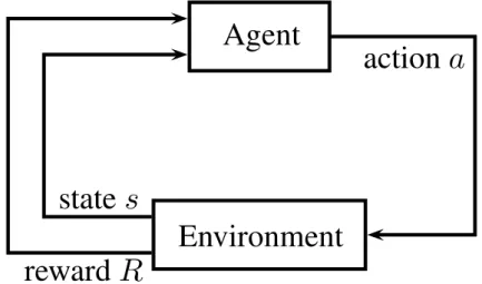
2.1 An illustration of the reinforcement learning framework. . . 10
3.1 A screenshot of a portion of the Ms. Pac-Man environment. . . 50
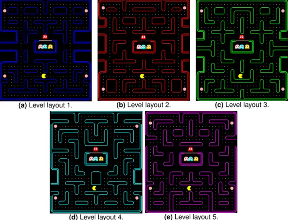
3.2 Initial level layouts for the Ms. Pac-Man environment. Each layout is used for two levels. . . 52
3.3 A screenshot of the Marioenvironment. . . 55
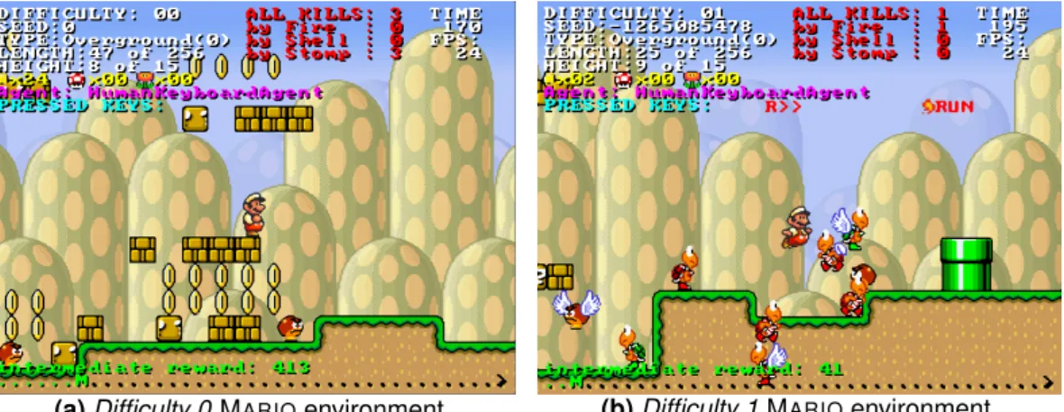
3.4 Example screenshots of the two Mariodifficulties. . . 57
3.5 A screenshot of the Carcassonne environment. . . 63
3.6 The set of tiles used in the game of Carcassonne. . . 66
5.1 A 3-block BlocksWorldstate observation example. . . 96
5.2 An example 3-block Blocks Worldstate. . . 99
6.1 Cerrla’s performance for the four BlocksWorldgoals. . . 120
6.2 Example policies created by Cerrlafor the four BlocksWorld goals. . . 122
6.3 The relationship between the number of Cerrla’s rules and the performance in BlocksWorld. . . 123
6.4 A comparison of Cerrla’s rate of learning on different sized BlocksWorldenvironments for theOnG0G1 goal. . . 123
6.5 A optimal OnG0G1 policy for 3-block Blocks World environ-ments produced by Cerrla. . . 124
6.6 A comparison of performance in BlocksWorldbetween using agent observations to simplify rules, and not using them. . . 127
6.7 An optimalOnG0G1BlocksWorldpolicy produced by Cerrla after 20,000 episodes without using simplification rules. . . 129
6.8 Cerrla’s performance using an alternative representation of
BlocksWorld. . . 129
6.9 Cerrla’s performance in a stochastic BlocksWorld. . . 131
6.10 Cerrla’s performance for the three goals in Ms. Pac-Man. . . 134
6.11 Example policies created by Cerrlafor the three Ms. Pac-Man goals. . . 135
6.12 The relationship between the number of Cerrla’s rules and the performance in Ms. Pac-Man. . . 136
6.13 Cerrla’s performance for the three goals in an alternative rep-resentation of Ms. Pac-Man. . . 138
6.14 Example policies created by Cerrla for the three goals of an alternative representation of Ms. Pac-Man. . . 139
6.15 Cerrla’s performance on theTen Levelsgoal when seeded with aSingle Levelpolicy in the Ms. Pac-Man environment. . . 140
6.16 The hand-coded rules used to seed Cerrla. . . 141
6.17 Cerrla’s performance on theSingle Levelgoal using the seeded rules from Figure 6.16 in the Ms. Pac-Manenvironment. . . 142
6.18 Cerrla’s performance for the two difficulty goals in Mario. . . 144
6.19 ExampleDifficulty 0Mario policy. . . 145
6.20 ExampleDifficulty 1Mario policy. . . 146
6.21 The relationship between the number of Cerrla’s rules and the performance for the two Mariogoals. . . 147
6.22 Cerrla’s performance on the Difficulty 1 goal when seeded with aDifficulty 0policy in the Marioenvironment. . . 148
6.23 Cerrla’s performance for the various goals of Carcassonne. . 153
6.24 ExampleSingle PlayerCarcassonne policy. . . 154
6.25 Example Cerrlavs. Random Carcassonne policy. . . 155
6.26 Example Cerrlavs. Static AI Carcassonne policy. . . 156
6.27 Example Cerrlavs. CerrlaCarcassonne policy. . . 156
6.28 Example Cerrlavs. 3 Static AI Carcassonne policy. . . 158
6.29 Example Cerrlavs. 3 CerrlaCarcassonne policy. . . 158
6.30 Example Cerrlavs. 5 Static AI Carcassonne policy. . . 159
6.31 Example Cerrlavs. 5 CerrlaCarcassonne policy. . . 159
6.32 The relationship between the number of Cerrla’s rules and the performance in Carcassonne. . . 161
List of Figures xiii
6.33 Cerrla’s performance when seeded withSingle Playerbehaviour for the Carcassonne Cerrlavs. Static AI goal. . . 162
List of Tables
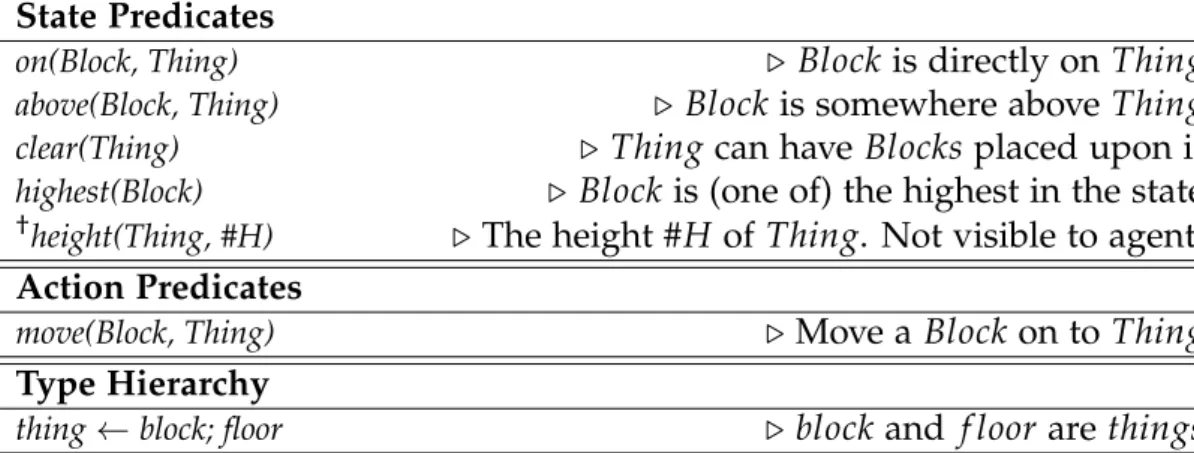
3.1 Predicate definitions for Blocks World. . . 47
3.2 Predicate definitions for Ms. Pac-Man. . . 53
3.3 Predicate definitions for Mario. . . 58
3.4 Terrain scoring in Carcassonne. . . 65
3.5 Predicate definitions for Carcassonne. . . 67
6.1 Cerrla’s performance for the BlocksWorldgoals. . . 120
6.2 Cerrla’s performance for different sizes of BlocksWorld en-vironments. . . 124
6.3 A comparison of performances for various RRL algorithms us-ing the BlocksWorldenvironment. . . 126
6.4 Comparison of performance between using and not using sim-plification rules in BlocksWorld . . . 128
6.5 Cerrla’s performance using an alternative representation of BlocksWorld. . . 130
6.6 Cerrla’s performance in a stochastic BlocksWorld. . . 131
6.7 Cerrla’s performance for the Ms. Pac-Mangoals. . . 133
6.8 Cerrla’s performance using an alternative representation of Ms. Pac-Man. . . 137
6.9 Cerrla’s performance when seeded with initial rules for the Ms. Pac-ManTen Levelsgoal. . . 141
6.10 Cerrla’s performance on theSingle Levelgoal using the seeded rules from Figure 6.16 in the Ms. Pac-Man environment. . . 141
6.12 Cerrla’s performance when seeded with initial rules for the
MarioDifficulty 1goal. . . 149 6.13 Cerrla’s performance for the various Carcassonne goals. . . 152 6.14 Cerrla’s performance when seeded withSingle Playerbehaviour
List of Acronyms
AI Artificial Intelligence
CEM Cross-Entropy Method
CERRLA Cross-Entropy Relational Reinforcement Learning Agent DP Dynamic Programming
EA Evolutionary Algorithm
GA Genetic Algorithm
GGP General Game Playing
ILP Inductive Logic Programming
JESS Java Expert System Shell KL Kullback-Leibler
LCS Learning Classifier System
LHS Left-Hand Side
LOMDP Logical Markov Decision Process
MDP Markov Decision Process
ML Machine Learning
POMDP Partially Observable Markov Decision Process
RHS Right-Hand Side
RLGG Relative Least General Generalisation
RMDP Relational Markov Decision Process
RRL Relational Reinforcement Learning
SARSA State-Action-Reward-State-Action
TD Temporal Difference
Publications
The following papers have been published throughout the course of this research:
Sarjant, S. (2013). A Direct Policy-Search Algorithm for Relational Rein-forcement Learning. In New Zealand Computer Science Research Student Con-ference (NZCSRSC) 2013.
Sarjant, S. (2012). Using the online cross-entropy method to learn rela-tional policies for playing different games. InNew Zealand Computer Science Research Student Conference (NZCSRSC) 2012.
Sarjant, S., Pfahringer, B., Driessens, K., Smith, T. (2011) Using the on-line cross-entropy method to learn relational policies for playing different games. In Computational Intelligence and Games (CIG), 2011 IEEE Conference on, pp. 182–189. IEEE.
Sarjant, S. (2011). CERRLA: Cross-entropy relational reinforcement learn-ing agent. In New Zealand Computer Science Research Student Conference (NZCSRSC) 2011.
Sarjant, S. (2010). Cross-entropy relational reinforcement learning. InNew Zealand Computer Science Research Student Conference (NZCSRSC) 2010.
1
Introduction
Look around. What do you see? Perhaps a computer monitor, sitting on a desk before you. Perhaps a collection of pages bound together with ink printed upon them. You may even see other people, doing whatever it is that they’re doing. You are probably reading this thesis because it has some meaning to you and your goal is to understand the information contained within. Reading a thesis (or any written document), involves relatively few actions. Turning the pages (or scrolling, if digital) and reading the infor-mation in front of you is basically all you need to do, perhaps occasionally looking up a cited paper that interests you. You will continue to read and turn pages until you have achieved your goal, whether that is to read the entire thesis, or just find the ‘juicy parts.’
The above scenario could be represented as a Relational Reinforcement Learning (RRL) problem: there is a collection of objects (tangible and in-tangible) and relations between those objects (e.g. contains(thesis, page1) is a relation that states that the object thesis contains the object page1). An ‘agent’ (i.e. the reader) can act upon these objects with the intent of achiev-ing a goal such as readachiev-ing the entire thesis (e.g.turnPage(thesis, page1, right-Hand) causes the agent to turn page1 in thesis with its rightHand), prefer-ably achieving that goal in a minimal amount of time. For example, some actions could be turnPage(thesis, page1, rightHand), readPage(thesis, page1, reader), makeCoffee(reader, mug), etc. In this scenario, every second spent reading the thesis is a second not used for other enjoyable activities,1which
could be represented numerically as a ‘reward’ of−1 per second with per-haps some large positive reward upon completing reading. Hence, the quicker an agent completes reading the thesis, the better the accumulated reward.
But how does an agent formally represent thesis-reading behaviour? Some approaches include:
1. A naive approach is to define the appropriate actions to perform for every possible state of thesis reading (e.g. per page, per thesis, per reading-format, etc.), but this approach is not generalisable and rep-resentation grows exponentially larger with the number of possible objects and relations involved in the thesis-reading problem.
2. A better approach is to define some form of abstraction, such that given a rough description of a state, the agent knows which action leads to maximal reward. This still requires the agent to learn which actions are best in what state, but the abstraction allows it to represent this information much more compactly than the first approach. 3. An even more general approach is to define some simple rules for
reading the thesis: read the page until it is completed, then move on to the next page. This behaviour is the implicit result in the prior two approaches, but it skips the first steps of explicitly representing which actions have the greatest value.
The algorithm developed in this research attempts to learn behaviour for solving a problem using the third approach. The problem with this ap-proach is that the algorithm needs to be able to create useful behaviour without explicitly learning per state which actions lead towards the great-est reward.
Before explaining the formal goal of this research, the following section provides a broad overview of the fields that it is based within.
1.1 Research Fields 3
1.1 Research Fields
1.1.1 Artificial Intelligence
The field of RRL is based within the broad field of Artificial Intelligence (AI). AI is a field within computer science that is concerned with the de-velopment of intelligent machines. This is a broad definition, as intelligence covers a wide range of behaviour and is difficult to formally define. There have been many definitions of AI, but they generally define AI as “anagent or system that ‘thinks’ and acts in a rational or human manner” (Russell and Norvig, 2003). Initially, early AI researchers were optimistic regarding how soon human-level intelligence AI was going to be developed, but this proved to be much more difficult than anticipated. AI research gravitated towards specialised applications (e.g. an AI that only plays Chess, or filters spam, etc.), but lately research has begun to return towards creating AI that can perform multiple tasks effectively.
1.1.2 Machine Learning
Machine Learning (ML) is a branch of AI concerned with learning solutions to problems when they are encountered, rather than simply acting out a rigid behaviour. A famous definition of ML by Tom Mitchell is:
A computer program is said to learn from experience E with respect to some class of tasks T and performance measure P, if its performance at tasks in T, as measured by P, improves with experience E(Mitchell, 1997).
That is, if a program’s performance increases after being provided with experience, it is said to be capable of learning. ML techniques can be broadly divided into three separate subfields: supervised learning (learning a model from labelled training data), unsupervised learning (learning the structure of unlabelled data), and reinforcement learning (learning which actions to take to maximise numerical reward).
1.1.3 Reinforcement Learning
Reinforcement Learning (RL) is a form of ML in which an agent seeks to maximise a numerical reward by performing actions within an environment.
Actions are selected by using the current observed stateas an input to the agent’s policy, which outputs the actions the agent takes. RL differs from supervised learning in that the ‘correct’ action is never explicitly stated; an agent only ever receives a numerical reward, and this reward may not even be received directly after an action is taken. For example, when playing a game such as Chessor Checkers, a player only receives a single reward at the end of a game of eitherwin (+1),loss (-1), ordraw (0). The actions per-formed throughout the game contributed to this reward, and so an agent must learn a policy that outputs an effective combination of actions and achieves the greatest reward.
1.1.4 Relational Reinforcement Learning
Relational Reinforcement Learning (RRL) is the name given to RL per-formed within environments represented asfirst-orderobjects and relations between the objects. The relational representation allows a flexibility in the state and action descriptions that otherwise could not be achieved with standard reinforcement learning. A relational state can be composed of any number of objects and relations and the number of actions available to the agent also varies based on the objects and relations present. How-ever, this flexibility also results in an enormous (even infinite) number of possible states, complicating the learning process. Since its conception in 1998 (Dˇzeroski et al., 1998), numerous algorithms have been developed for solving RRL problems, though many have only been tested upon the benchmark BlocksWorldenvironment (Section 3.3). The majority of RRL algorithms use value-based approaches to represent expected reward for relational states. An agent’s behaviour is then extracted from these values by greedily performing actions with the largest expected reward.
1.2 Motivation and Goal
The goals of this research are to:
• Develop a new RRL algorithm that learns effective behaviour using direct policy search methods.
• Investigate the utility of the algorithm over a range of environments of differing sizes and formats.
1.2 Motivation and Goal 5
The decision to learn behaviour via direct policy search methods was made because firstly, there already exists a large number of different value-based approaches with varying levels of performance, and secondly, direct policy search methods do not need to learn the expected value of actions, and so are unaffected by changes in the reward function (by changing the size of the environment, or as a result of modified behaviour).
The proposed approach for the algorithm is to utilise the Cross-Entropy Method (CEM), a distribution-based optimisation method, to generate rule-based policies by storing relational rules within distributions and generat-ing policies by randomly samplgenerat-ing rules, where the probability of samplgenerat-ing a rule is increased with the rule’s usefulness. This approach allows the al-gorithm to automatically explore different policies as random samples, but gradually modifies the sampling distribution such that the generated poli-cies result in a greater reward. The CEM has been shown to be effective in a range of different problems, so this research will investigate an application of the CEM towards learning behaviour in RRL problems.
The second goal is concerned with applying RRL algorithms to larger prob-lems. Most RRL algorithms are primarily evaluated on the benchmark ‘Blocks World’ environment, which is ideal for demonstrating the core challenges of RRL, but remains an artificial ‘toy’ problem. This research will be tested both upon Blocks World problems, and larger problems with more complex interactions. Games provide excellent environments for this purpose because they have a set of well-defined gameplay rules, an obvious reward function (the score), object-orientated elements, com-plex and often random gameplay elements, and are relatable to humans. To demonstrate the algorithm’s ability to learn behaviour over a range of environments, three different games will be used as testbeds for the algo-rithm.
Regarding additional requirements, the algorithm should be able to: • Learn behaviour quickly. If it takes a long time to learn effective
behaviour, then the algorithm’s usefulness is reduced.
• Learn effective behaviour without guidance from an external ‘expert.’ It needs to be able to infer its own useful rules when only provided with observations on the environment and the language in which the
environment is represented.
• Represent the behaviour in a comprehensible manner, such that it is obvious to a human viewer how the policy selects its actions.
1.3 Thesis Structure
The remainder of this thesis is structured as follows:
• Chapter 2 describes the fundamental concepts behind this work and presents an introduction to the existing related work. These include an introduction to Reinforcement Learning (RL) and a brief descrip-tion of the various approaches for RL algorithms, a formal descripdescrip-tion of Relational Reinforcement Learning (RRL) and a summary of the al-gorithms developed for it, and an overview of various AI applications to playing games.
• Chapter 3 formally defines the syntax that is used by the algorithm and the specification language that each environment is represented in. Each of the four environments used within this research are also formally defined here.
• Chapter 4 presents a full explanation of the algorithm developed in this research, the Cross-Entropy Relational Reinforcement Learning Agent (Cerrla). This chapter primarily describes how the algorithm utilises the CEM to explore and exploit the relational rules that are created by the algorithm (detailed in Chapter 5).
• Chapter 5 describes how the algorithm extracts information about the environment to create and explore relational rules for acting within the environment. This includes initial rule creation, specialisation conditions, and inferring simplification rules for removing redundant rule conditions and reducing the effective number of rules the algo-rithm needs to search.
• Chapter 6 presents evaluation results for Cerrla on the four envi-ronments defined in Chapter 3. These results include the perfor-mances on different environmental goals, the effects of alternative environmental representations, and comparisons to other learning al-gorithms.
1.3 Thesis Structure 7
• Finally, Chapter 7 discusses the algorithm presented in this disserta-tion and summarises the work presented in previous chapters, pre-senting conclusions on the outcome of the work and identifying pos-sible future work.
A list of the figures, tables, algorithms, acronyms and publications can be found directly after the table of contents.
2
Background
The previous chapter introduced the concepts that are necessary for un-derstanding the aim of this research. This chapter should give the reader a solid understanding of various solutions for Relational Reinforcement Learning (RRL) and how this research fits into the RRL context. This chap-ter describes the current state of RRL research, but before that, it describes the key concepts and existing approaches for Reinforcement Learning (RL) problems as many RRL algorithms are inspired by propositional RL algo-rithms and ‘lifted up’ to the relational setting. Three of the testing envi-ronments used in this research are games, so we also look at various AI applications towards playing games.
We begin by firstly reviewing the RL framework and existing approaches towards solving RL problems (Section 2.1). Section 2.2 then formally de-fines RRL, describing how RL aspects can be ‘lifted’ to the relational set-ting. We also examine existing RRL algorithms, investigating their relation to existing RL algorithms and their strengths and weaknesses. Section 2.4 outlines the various reinforcement learning and other related learning al-gorithm approaches that have been applied to games. Finally, Section 2.5 summarises the content presented in this chapter and discusses how it ap-plies to the algorithm presented in the following chapters.
2.1 Reinforcement Learning
Reinforcement Learning (RL) is a method of machine learning in which a learningagentseeks to maximise a numericalreward by interacting with its environment(Sutton and Barto, 1998; Kaelbling et al., 1996). An agent inter-acts with anenvironment in discrete time steps tand at every time step the environment provides a description of the currentstateof the environment st to the agent. The agent then selects an action at to perform, which is re-turned to the environment. This causes the environment state to transition to another state st+1 and produce numerical feedback about the quality
of the state transition. The goal of the agent is to maximise the overall feedback received. Figure 2.1 presents an illustration of the reinforcement learning loop.
Example 2.1.1. For example, an agent’s interaction with a generic environ-ment described by a set of numerical features is as follows:
Agent
Environment
action
a
state
s
reward
R
2.1 Reinforcement Learning 11
Environment: At time step 0, you are in state 23. Feature 2, 6 and 9 are true. You have 4 possible actions.
Agent: I’ll take action 3.
Environment: You receive a reward of 2. At time step 1, you are now in state 16. Feature 2, 3 and 5 are true. You have 6 possible actions.
Agent: I’ll take action 1.
Environment: You receive a reward of−4. At time step 2, you are now in state 3. Feature 9 is true. You have 2 possible actions. ..
. ...
Unlike most forms of machine learning, the ‘correct’ action is not known to the agent; there is only a numerical reward. This is one of the main chal-lenges in RL: the problem of exploration vs. exploitation. The agent needs to exploitactions that it knows produce high reward, but also needs toexplore other actions to check if they produce even higher reward. A greedy agent would simply exploit the first strategy that provides reward, which is prob-ably not optimal, therefore a learning agent needs some sort of exploration strategy. This is complicated by the fact that the learning is performed online within the environment, meaning the environment is a ‘black box’; states can only be accessed by taking the necessary actions to get to them. Offline learning allows an agent to select any state and perform an action, but this thesis will not cover this form of RL.
A comprehensive explanation of RL techniques can be found in Kaelbling et al. (1996), Sutton and Barto (1998), Szepesv´ari (2010), Bus¸oniu et al. (2010) and Wiering and van Otterlo (2012).
2.1.1 Markov Decision Process
Markov Decision Processes (MDP) (Bellman, 1956; Puterman, 1994) are an intuitive framework for representing reinforcement learning (Bertsekas and Tsitsiklis, 1996; Kaelbling et al., 1996; Sutton and Barto, 1998), decision-theoretic planning (Boutilier and Dearden, 1994) and other stochastic state-driven domains. A Markov Decision Process (MDP) represents a problem as a set of connected states that are navigated by selecting actions. Each transition between states has a probability and a reward associated with it and the goal of the agent acting within the MDP is to maximise the amount
of reward received by selecting an appropriate action at each time step.
Definition 2.1.1(Markov Decision Process (MDP)). Formally, an MDP is a tuple M =hS,A,T,Ri, defined as:
• A finite set of states S, • A finite set of actions A,
• A transition function T : S×A×S→[0, 1], • A reward function R: S×A×S→R.
For every states ∈S, the agent is provided with the set of actionsA(s)that can be performed for the current state. When action a is applied in state s, the transition function defines the probability of transitioning to state s0 ∈ S as T(s,a,s0). Every T(s,a,s0) ≥ 0 and T(s,a,s0) ≤ 1, and for every s and a, ∑s0∈ST(s,a,s0) = 1. A numerical reward is also produced using
R(s,a,s0), where the value may be any real numerical value.
The agent’s job is to learn a policy π : S → A (or a probabilistic policy π : S×A→ [0, 1], but this work focuses on the deterministic form), which maps states to actions (π(s) = a). The policy is the agent’s method of interaction with the environment and the agent’s goal is to create a policy that receives maximal reward when interacting with the environment. An MDP may also specify a distribution of starting states and/or termi-nal states. The starting states define the first state an agent may begin in when learning begins, and terminal states define states in which theepisode is complete (either because the agent reached the goal, or cannot act any-more).
A core aspect of MDPs is the Markov assumption which states that: “the current state provides enough information to make an optimal decision.” This clause restricts the number of environments that fit into the MDP framework, as environments that are not fully-observable (e.g. hidden-information domains such as Poker) do not fit this assumption. Nonethe-less, the MDP framework provides an approximate description for such environments.
2.1 Reinforcement Learning 13
Partially Observable Markov Decision Process
A Partially Observable Markov Decision Process (POMDP) is a generali-sation of an MDP where the agent does not have access to all state ob-servations (Kaelbling et al., 1998). A POMDP assumes there is an MDP modelling the environment, but the agent only has access to a partial ob-servation of it. Many real-world environments are only partially observ-able, due to an element of randomness, imperfect sensors, the presence of other ‘black box’ agents, etc. The three game environments presented in the next chapter could all be classified as POMDPs because each environ-ment contains competing agents with unknown behaviour (as well as other unknown elements of the environment).
Definition 2.1.2(Partially Observable Markov Decision Process (POMDP)).
Formally, a POMDP is a tuple hS,A,O,T,R,Ωi, such that S,A,T,R are defined as usual, Ois a set of observations upon the actual state S, andΩ is the observation function Ω : S×A×O → [0, 1] defining a probability distribution over observations received given an action and resulting state. A POMDP can be treated as an MDP, but the learning algorithm may need to make use of a belief state to probabilistically infer what fully-observed state the agent is in. Without knowing what state the agent is actually in, calculations that make use of previous rewards cannot be effectively utilised.
2.1.2 Solving Markov Decision Processes
The most obvious approach to solving reinforcement learning problems is to maintain a value function Vπ = S → R that returns an expected reward
for states if following policyπ. The goal is then to create a policyπ∗ such that the value function Vπ∗ achieves the maximal possible reward in every
state. Value functions are defined as: Vπ(s) = E[
∞
∑
t=0
γtR(st,π(st),st+1)] (2.1)
where 0 < γ < 1 (usually γ = 0.9) to prevent the sum of rewards going to infinity in environments without a terminal state. This definition states that the value of a state while following policy π is equal to the expected reward of all following states.
A value function can also be recorded for every action a in state s, known as the Q-functionQπ(s,a)(Quality-function). Instead of estimating the
ex-pected reward for every state, the Q-function estimates the exex-pected reward for every state-action pair:
Qπ(s,a) = E[
∞
∑
t=0
γtR(st,a,st+1)] (2.2)
The values of each function can be estimated by recording an average of the rewards following each state, or for the Q-function, the rewards following each individual action taken from the state. As the number of times the state value is updated approaches infinity, the estimated value becomes closer to the true value of the state (or state-action).
Existing Value-Based Algorithms
Reinforcement learning problems can be solved with two main approaches: learning (or being provided with) a model of the environment and using dynamic programming (DP) to iteratively determine the optimal policy, or learn the values for states withtemporal-difference learning.
Dynamic Programming (DP) computes the value of states by iteratively propagating rewards back through the MDP using the known transition and reward functions. While not strictly part of RL, DP provides an alter-native method of solving MDPs. DP approaches are guaranteed to find the optimal policy because the optimal value function V∗ can be represented as the following equation (using theinfinite horizon metricas the optimality metric, Equation 2.1): V∗(s) = max a∈A s
∑
0∈S T(s,a,s0)R(s,a,s0) +γV∗(s0) (2.3)which can be used to calculate the optimal policy π∗ (by always selecting the action that leads to the greatest reward). This equation is known as the Bellman optimality equation(Bellman, 1956) which states that the value of a state s is equal to the immediate reward received R(s,π(S),s0) following the current policy π plus the average expected reward for the following statesV(s0) with respect to their transition probability T(s,a,s0).
it-2.1 Reinforcement Learning 15
eration (Howard, 1960). Value iteration computes the optimal value func-tion using the Bellman optimality equafunc-tion to propagate rewards between states. Policy iteration switches between recomputing the value function and improving the current policy based on the recomputed value function, eventually converging to an optimal solution. Both methods are guaran-teed to find the optimal solution as each iteration always improves the quality of the agent’s behaviour.
The main problem with dynamic programming approaches is that the tran-sition and reward functions are usually not known. In this case, an agent must learn the transition and reward functions if it is to use DP techniques (known as indirect RL). The DYNA architecture (Sutton, 1991) combines Q-learning and DP by learning a model while concurrently acting in the environment. The learned model is then used to generate extra learning ex-perience by simulating extra interaction with the environment. Prioritised Sweeping (Moore and Atkeson, 1993) improves upon this idea by prioritis-ing updates of the learned model to areas where the change in observed values is greatest.
The other option for value-based learning is Temporal Difference (TD) learning (directRL). TD learning incrementally updates the expected value of states using the immediate observed reward and the estimated rewards of future states (known asbootstrapping). TD(0) (Sutton and Barto, 1998) is the simplest form of TD learning. At every time step, the algorithm can update the value of states using the observed rewardrand value estimate for the following state V(s0).
Vk+1(s) =Vk(s) +α
r+γVk(s0)−Vk(s)
(2.4) where α ∈ [0, 1] is the step-size (or learning rate) parameter that controls how much values get updated. Like Equation 2.3, the value of a state depends on following states, but instead of a weighted average of all fol-lowing states, TD learning only uses the observed transition to update the value.
To avoid converging to a single, possibly sub-optimal strategy and to search for potentially better strategies, the agent needs to occasionally explore ac-tions that are not simply selecting the action that leads to the largest ex-pected reward. The simplest approach is e-greedy explorationwhich selects
a random action with probability e, otherwise it selects a greedy action. A problem with this strategy is that it performs unnecessary exploration in the later stages of learning and that random actions can lead to highly undesirable states. Another approach is to useBoltzmann exploration, which uses a ‘temperature’ variableTand the current Q-value estimates to control action selection: P(a) = e Q(s,a) T ∑a0∈A(s)e Q(s,a0) T (2.5) where P(a) defines the probability of selecting action a. The temperature T is gradually decreased to reduce exploration and increase exploitation. Q-learning is a popular variation of TD learning, which learns Q-values for states in a similar manner to TD(0) (Watkins and Dayan, 1992). The Q-learning update equation is:
Qk+1(s,a) = Qk(s,a) +α r+γ max a0∈A(s0)Qk(s 0 ,a0)−Qk(s,a) (2.6) This equation is nearly identical to Equation 2.4, except it utilises the max operator to select the best estimated value for the next state. Because of this operator, Q-learning is anoff-policy algorithm, because it only updates Q-values with the best estimated Q-values. Anon-policyvariation of Q-learning is SARSA: Qk+1(s,a) =Qk(s,a) +α r+γQk(s0,π(s0))−Qk(s,a) (2.7) Note that the SARSA equation uses the policy’s output action for Q-value updates instead of the max operator. Both techniques are guaranteed to converge to the optimal solution given infinite samples, but SARSA re-quires that the algorithm eventually ceases to explore.
An alternative value-based class of algorithms areactor-criticmethods (Wit-ten, 1977; Barto et al., 1990; Konda and Tsitsiklis, 2003). Actor-critic meth-ods maintain an explicitly separate policy to the value function. The policy is known as theactorbecause it selects the actions and the value function is known as thecriticbecause it criticises the actions performed by the policy. The criticism is in the form of TD error:
2.1 Reinforcement Learning 17
If positive, the critic strengthens the probability of selecting the action and vice-versa. The following update equation defines thepreferenceof selecting actionat in a given statest(where actions with a higher preference are more likely to be selected):
p(st,at)← p(st,at) +βδt (2.9) where β is a step-size parameter determining how much the value is up-dated. Note that together, Equation 2.8 and 2.9 are very similar to the value and Q-learning update equations.
2.1.3 Generalisations and Abstractions
In small environments, maintaining a table of values for every state (or every state-action in the case of Q-learning) is enough to learn an optimal policy in reasonable time. But for larger or more complex environments, the size of the table grows exponentially larger and becomes difficult to manage, both in terms of memory usage and value-propagation, resulting in a slower rate of learning. The following subsections define core general-isations or abstractions that can be applied to RL techniques to reduce or approximate the state space of an environment.
Value Function Approximation
Instead of recording the expected value of each state directly, a parame-terised function can be used to represent the value function of states (Bert-sekas and Tsitsiklis, 1996; Sutton and Barto, 1998; Bus¸oniu et al., 2010). By representing the expected reward of states as a function, the agent only needs to learn the function, which allows it to estimate the expected value of unseen states as well. This is known as learning a regression model for predicting a state’s estimated value. A learned model takes a state (and action) as input and outputs the expected value of the state, in accordance with the model.
Learning a regression model is a well-understood problem in supervised learning, but the key difference with learning a regression model in RL is that learning is performed online, with non-stationary expected state re-wards. Therefore, the regression model needs to be able to incorporate new examples and changes to the existing data as the expected values for states
change. This can be achieved either by using anincremental regression model or learning function approximators with batches of examples (known as batch RL). Theoretically, any supervised learning algorithm can be used as a function approximator, either in an incremental or batch fashion, e.g. lin-ear function approximation(Samuel, 1967; Utgoff and Precup, 1998), decision trees (Chapman and Kaelbling, 1991; Wang and Dietterich, 1999), neural networks(Tesauro, 1994; Bertsekas and Tsitsiklis, 1996), evolutionary methods (Whiteson and Stone, 2006),kernel-based methods (Ormoneit and Sen, 2002) andsupport-vector machines(Dietterich and Wang, 2001).
Direct Policy Search
Most approaches in RL learn an optimal policy by maximising the expected value of actions, where the expected value is either computed from a table of values or a value-function approximation. Direct policy search com-pletely skips the need for expected values by instead computing a policy directly. Value functions are typically larger than the policies generated from them, and usually encode more information than the policy requires. For example, given a simple ‘corridor’ environment of length ten, where the actions available are to goleftor right, and the goal is to be in the
far right edge of the corridor, a value function needs to represent the ex-pected value for each state and each action, whereas a policy simply needs to saygo right.
An obvious method of learning policies is to treat RL as asupervised learning problem by gathering a number of good examples (goal-achieving) and use them as input to a classification model. This method transforms RL into a series of supervised learning tasks (Barto and Dietterich, 2004; Langford and Zadrozny, 2005). Lagoudakis and Parr (2003) use anapproximate policy iteration(API) framework that uses policy rollouts(Boyan and Moore, 1995) to create a number of policy samples as input for a classifier algorithm. P-learning (Dˇzeroski et al., 2001) is partially a value-function approxima-tion method as it maintains the same structure as Q-learning, but instead of encoding the expected state values, it simply encodes whether an action within a state is optimal or not (1 for optimal, 0 for non-optimal). This usu-ally results in a smaller representation of the state compared to Q-learning, and does not need to maintain the expected value of state-actions.
2.1 Reinforcement Learning 19
A policy gradient approach uses gradient-descent techniques to locate the optimal policy. By representing the policy such that a gradient can be defined for its parameters, the optimal policy can be found by using tech-niques such as hill-climbing. The REINFORCE algorithm (Williams, 1992) learns the policy gradient by repeatedly testing the policy against the en-vironment, then updating the weights of the policy through hill-climbing. A problem with this algorithm is that it is on-policy and can be relatively slow. Sutton et al. (1999a) extend the REINFORCE algorithm by combining it with function approximation to aid the policy gradient estimation and speed up the rate of convergence.
Baird and Moore (1999) present an alternative policy gradient method named VAPS (Value and Policy Search). The VAPS algorithm combines both value function approximation and policy search, allowing the agent to select actions using either technique. Wierstra and Schmidhuber (2007) adapt the actor-critic method to learn policy gradient critics in POMDP environments.
Policies can be generated through the use of an Evolutionary Algorithm (EA) (Holland, 1992; Goldberg, 1989), either by evolving the entire policy, or the individual rules that compose the policy (Moriarty et al., 1999). EA maintains a population of chromosomes, where the best chromosomes are mutatedto produce different chromosomes. EAs require two key factor for creating policies: 1) an evolvable policy representation, 2) an appropriate fitness function for the policies. The reward function typically serves as the fitness function (i.e. reward received for the episode). EAs have been combined with RL to evolve rule-based policies (Smith, 1983; Grefenstette et al., 1990) and neural networks (neuro-evolution) (Belew et al., 1992; Whit-ley et al., 1993; Moriarty et al., 1999).
An alternative application of EA is to learn parts of the policy and bring them together in combination. In these systems, learning is performed both on the overall structure of the policy and on the individual compo-nents that make up the policy. Learning Classifier Systems (LCSs) (Hol-land, 1995; Lanzi et al., 2000) use a EA and RL techniques to maintain a population of ‘if-then’classifiersthat map input to an action. The classifiers represent the agent’s policy, so when input is received, all classifiers with matching conditions activate. Every classifier has astrengthassociated with
it that records the expected reward (like value-based RL techniques) and that strength is also used as a fitness function for selecting classifiers for ge-netic mutation operations. Dorigo and Colombetti (1998) combine several LCSs hierarchically to learn behaviour for multiple subtasks.
The XCS classifier (Wilson, 1995) alters the LCS algorithm by using the ac-curacyof a classifier as the fitness function for genetic mutations instead of the strength. The accuracy of a classifier is the error between the classifier’s expected reward and the actual reward received. The fitness of a classifier is a function of the inverse error such that classifiers that accurately pre-dict the reward received are more favourable than those that simply have a high, but erroneous, expected reward. The ‘Hayekmachine’ (Baum, 1999) is similar to an LCS in that it maintains a collection of agents that bid on which actions to take, where agents that bid on high-quality actions receive a relative reward. This strategy allows each agent to focus its bids and rule learning on sub-problems within the environment. The rules each agent uses are created through evolutionary methods of mutation and random initial conditions.
Symbiotic, Adaptive Neuro-Evolution (SANE) (Moriarty and Mikkulainen, 1996) uses a neuro-evolution approach to learning behaviour by using sym-biotic evolutionto learn weights for individual neurons within a larger fixed-size neural network. Each neuron only learns a portion of the policy but they rely on other neurons to create effective behaviour. Neuro-Evolution of Augmenting Topologies (NEAT) (Stanley and Miikkulainen, 2002) is an extension to SANE that allows the topology of the network to change rather than using static-structure networks. Potter and De Jong (2000) define a rule-based form of symbiotic evolution, where each chromosome in the population represents a set of rules that only address a subset of the task. The Cross-Entropy Method (CEM) is a relatively recent optimisation algo-rithm similar to Learning Classifier Systems and Evolutionary Algoalgo-rithms (Rubinstein, 1997; De Boer et al., 2004). The CEM can be summarised in two steps: 1) Generate a number of random samples from the current dis-tribution of data, 2) Update the data disdis-tribution such that the best subset of the random samples (elite samples) are more likely to be sampled in the next iteration (i.e. minimise the cross-entropy distance between the current distribution and the observed elite samples). Applied to RL problems, it
2.1 Reinforcement Learning 21
can be used to generate a number of policies, the best of which are used to influence the sampling distribution such that they are more likely to be randomly sampled again. Although CEM has been applied to a multi-tude of different problems, this subsection only describes the applications of CEM to RL. Other applications include clustering (Kroese et al., 2007), control and navigation (Helvik and Wittner, 2001), DNA sequencing (Keith and Kroese, 2002), network reliability (Hui et al., 2005), and continuous optimisation (Kroese et al., 2006).
Mannor et al. (2003) demonstrate a simple application of CEM to a maze-traversing RL by representing the agent’s policy as an action distribution (e.g. move up, down, left, or right) for every location in the maze. The al-gorithm learns by generating N policy samples, testing them, and the best policy samples (elite samples) are used to update the sampling probabilities for every action distribution, such that favourable actions are more likely to be sampled. Chaslot et al. (2008) apply CEM towards playing the board game Goby using it to tune the parameters of aMonte-Carlo Tree Search al-gorithm, improving the results of the algorithm over the non-tuned learner. Szita and L ¨orincz (2006) apply CEM to the Tetrisvideo-game by represent-ing the policy as a vector of weights for features in the game. They also inject noise into the sampling process to reduce the likelihood of early con-vergence. Thiery and Scherrer (2009) improve upon this work by adding additional features and Kistemaker (2008) also applies CEM to learning to play Tetris.
Szita and L ¨orincz (2007) create rule-based decision-list policies for playing the Ms. Pac-Mangame by using the CEM to identify which rules are useful and what order they should be used in. Each decision-list policy is created from multiple rule distributions by sampling one rule from each distribu-tion where each distribudistribu-tion also has a probability of being included in the sampled policy. Each distribution contains the same ‘condition-action’ rules that use high-level actions for the agent’s behaviour (e.g. toDot,
fromGhost, etc. rather than directional movement). The order of the rules
in the policy is dependent on the order of the distributions. The sampled policies are also hierarchically structured such that multiple rules can be ac-tivated at once (e.g. Ms. Pac-Man can eat dots while avoiding ghosts). The algorithm evaluates a number of sampled policies and uses the best poli-cies (the elite polipoli-cies) to alter the rule distributions such that effective rules
are more likely to be included in later policies. The authors use predefined rules, but they also run experiments using (bounded) randomly generated rules. The research presented in this thesis was initially based upon this work and uses a similar (relational) method of acting in the Ms. Pac-Man environment.
2.1.4 Reinforcement Learning Summary
The above summary of algorithms shows that there already exist a large number of solutions for RL problems but all solutions have a common weakness: they can only learn behaviour in environments where the repre-sentation is a static set of features. In many cases this is sufficient, but often an environment will utilise a changing number of objects and relations be-tween objects. This can be dealt with by adjusting the state representation to represent all possible aspects of the environment but every additional object or relation can exponentially increase the number of features re-quired to model every possible state of the environment. The following section introduces Relational Reinforcement Learning (RRL), a subfield of RL in which an environment is represented as a collection of objects and relations, providing more freedom in expressing the environment state.
2.2 Relational Reinforcement Learning
Relational Reinforcement Learning (RRL) is a representational generali-sation of RL that expresses the environment as logical relations between objects and actions taken upon those objects (Dˇzeroski et al., 2001). Tra-ditional RL algorithms are based in propositional environments, where the structure of the states is fixed. But in more complex environments this form of state representation is not sufficient. States can be dynamically chang-ing, introducing new objects or removing old objects. RRL represents these object-based environments using first-order logic, both for observations on states, and for actions to take within states.
RRL is strongly based on the field of Inductive Logic Programming (ILP), a subfield of ML in which hypotheses are inductively learned from a set of logically-defined examples (Lloyd, 1993; Genesereth and Nilsson, 1987; Muggleton, 1991; Dzeroski, 2001). Examples are represented as sets of facts
2.2 Relational Reinforcement Learning 23
consisting of objects and relations, and additional information about the examples can be inferred using background knowledge to infer new facts. ILP’s expressive representation of facts is ideal for representing problems with a non-fixed number of features.
The syntax used in RRL is strongly based on ILP syntax, defined below (for a full definition, see Lloyd (1993), Genesereth and Nilsson (1987) or Dzeroski (2001)):
Definition 2.2.1 (Logic Programming Syntax). Each environment defines analphabetΓofpredicatesthat make up therelational state observations, a sep-arate set of predicates that make up the availablerelational actionsan agent can take, and a set of named objects (constants) that are present within the environment. Each predicate is instantiated with terms: either a constant, variable, orfunction. Constantsrepresent unique objects within the environ-ment, variables are placeholders for constants, and functions return a value when provided with argument terms. Anatom is a predicate that contains terms. A literal is a negated or non-negated atom. If an atom or literal does not contain any variable terms, it isgrounded. Asubstitutionis a set of assignments of terms to variables, where each variable is only assigned a single term.
The Herbrand base of Γ (HBΓ) is the set of all ground atoms that can be constructed with the state predicatesPS (and action predicates PA) and the constants C. AHerbrand interpretation is a subset of HBΓ.
The main advantage of this alternative representation is the flexibility in expressing facts about the environment. Where traditional RL defines a fixed set of attributes with which to represent the environment, RRL is able to describe any number of facts about any number of objects.
2.2.1 Relational Markov Decision Process
Relational environments are structured using the Relational Markov Deci-sion Process (RMDP) framework; an extenDeci-sion of the MDP framework seen in Section 2.1.1. There are multiple definitions of RMDPs (e.g. Wang et al. (2008), Croonenborghs et al. (2007), Kersting and Raedt (2004), Fern et al. (2006)), and we use the same one given in Croonenborghs et al. (2007):
is defined as the five-tuple M = hPS,PA,C,T,Ri, where PS is a set of state predicates, PA is a set of action predicates, and C is a set of constants. A ground state (action) atom is of the form p(c1, . . . ,cn) with p/n ∈ PS (p/n ∈ PA) and ∀i : ci ∈ C. A state in the state space S is a set of ground state atoms; an action in the action state A is a ground action atom. The transition function T and reward function R are defined as usual by T : S×A×S →[0, 1] and R: S×A×S→R.
The Herbrand base for an RMDP defines all the possible atoms used to describe a state, though not every atom is necessarily legal. Some combi-nations of constants could be infeasible for the current environment, and some combinations of atoms could represent illegal states.
Note that compared to an MDP definition, the RMDP definition is one which implicitly defines the state and action space, as it simply defines the components that compose the state and action space. Because states may have any number of facts, an explicit definition of the state space is impossible because the number of states may be infinite. However, this flexibility is also the primary benefit of RRL as there are no restrictions on which objects or facts are present.
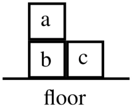
An example environment commonly used in RRL and planning algorithms is the BlocksWorldenvironment (Slaney and Thi´ebaux, 2001). It consists of a number of blocks stacked on top of one-another, and a floor upon which to stack the blocks. A full definition of BlocksWorldcan be found in Section 3.3. A possible RMDP for a small BlocksWorldis as follows:
Example 2.2.1(Blocks World RMDP). Defining the Blocks World alpha-bet as PS = {on/2,clear/1} (such that on takes two arguments and clear takes one argument), PA = {move/2}, and C ={a,b,c,d,e,f,fl}, a possible state could bes1 ={clear(a), on(a,b), on(b,d), on(d,e), on(e,c), on(c,fl)}. s1
defines a single stack of blocks, witha on top and a single action A(s1) = {move(a,fl)}, which moves blockato thefl, resulting in states2 (with some
probability given by T(s1,a1,s2) and reward given by R(s1,a1,s2)). Note
that the block f is not present in the state, because relational states do not necessarily need to include every object.
2.2 Relational Reinforcement Learning 25
2.2.2 Benefits and Challenges of RRL
The relational format has several benefits over the propositional represen-tation in RL:
• States may contain any (legal) combination of objects and relations. Each state is a snapshot of the current state of the environment, with information about each object and the relations between the objects composing the state description.
• Actions can directly relate to the objects in the state. In proposi-tional representations, actions may only implicitly relate to objects (e.g. openDoor1, openDoor2), whereas relational representations ex-plicitly define the objects required for the action (e.g. open(door1), open(door2)).
• The first-order representation allows agents to leverage variables to generalise across objects. This is one of the most important abstrac-tions of RRL as it allows an agent to define generalised behaviour by acting upon objects that satisfy the relational properties, rather than defining behaviour for each individual object.
• Background knowledgecan be provided by the environment that defines rules to automatically infer new facts and define illegal states.
However, it also introduces a number of new challenges as well:
• The flexibility of state descriptions results in an enormous number of possible states, even when using background knowledge to remove illegal states. This makes brute-force state-action tables impractical, so abstractions must be used to create effective learners.
• Measuring distances between first-order states is more difficult than propositional representations due to the variable number of facts and objects present between states.
• First-order reasoning is generally slower than propositional methods. van Otterlo and Kersting (2004) provide more detail about the challenges faced by RRL.
2.3 Existing RRL Algorithms
This section briefly summarises the distinct approaches that have been used to learn behaviour within RRL problems, many of which are based on tech-niques presented in Section 2.1. Refer to the following for comprehensive surveys on RRL techniques: van Otterlo and Kersting (2004), Tadepalli et al. (2004), van Otterlo (2005), van Otterlo (2009), or the most recent sur-vey Wiering and van Otterlo (2012).
There are three primary approaches towards solving RRL problems: static generalisation methods, which provide the environment generalisations for value-based methods prior to learning (model-based methods also fall into this approach);dynamic generalisation methods, which create generalisations for the environment and use value-based methods for learning; and policy search methods, which create policies directly, thereby removing the need to generalise the states of the environment. This section will describe each approach and discuss existing algorithms that have been created for each approach.
Static Generalisation Methods
Static generalisation methods provide an abstraction of the state-actions table such that each entry represents a partial, possibly variable, abstract state. Standard value-based learning techniques are then used to locate the optimal policy for the abstract state-action table. This includes algo-rithms such as CARCASS (van Otterlo, 2004), Logical Markov Decision Process (LOMDP) framework (Kersting and Raedt, 2004), and Relational Q-learning (rQ) (Morales, 2003).
Dynamic Generalisation Methods
One of the earliest algorithms for solving RRL problems was the RRL-system (Dˇzeroski et al., 2001; Driessens, 2004), which combined RL and ILP to define a general system for learning Q-functions in RRL problems. The basic idea of the algorithm is to gather a collection of state-action examples over the course of an episode, updating the Q-value of each state-action pair using Q-learning, then use the examples as input into a relational regression classifier to produce a compact classifier that predicts the Q-value for a state-action.
2.3 Existing RRL Algorithms 27
The first implementation of the RRL-system used the TILDE-RT relational decision-tree learner (Blockeel and De Raedt, 1998) to represent the Q-function (denoted as the Q-RRL algorithm). Each node contains a test consisting of a single query that may share variables with other nodes and the leaves of the tree contain Q-values. The main problems with Q-RRL is that it needs to store each state-action example in order to learn an accu-rate function approximator and that it builds a new tree after every episode (which takes increasingly longer as the set of examples grows). Driessens (2004) created several incremental algorithms that remove the need to store each example: RRL-TG, an incremental relational decision-tree learner that learns trees of the same structure as the TILDE-RT (Driessens et al., 2001); RRL-RIB, an instance-based learner that uses a set of well-chosen, expe-rienced state-action instances to calculate distances for state-action pairs (Driessens and Ramon, 2003). This distance metric needs to be defined beforehand by the user. RRL-KBR uses graph kernels and Gaussian pro-cesses as a regression technique for approximating the value of state-action pairs (Driessens et al., 2006).
The RRL-TG algorithm was also extended into several different directions: TGR incorporates tree-restructuring operations to mitigate the effects of ineffective splits or tests by pruning sub-trees or revising the split (Ramon et al., 2007). TGR is also able to capably deal with concept drift (goal of the environment changes). Driessens and Dˇzeroski (2005) combined RRL-TG and RRL-RIB to create Trendi, a tree-based model with instance-based representation for the leaves of the tree.
The NPPG algorithm (Kersting and Driessens, 2008) uses policy-gradient techniques to optimise a weighted sum of regression models created in stage-wise optimisation during learning. The regression models are cre-ated usingboosting: each regression model is created to cover the examples previous models do not adequately cover. In the relational setting, this can mean creating a model for previously unseen features of the state. Each model is also weightedby a value that is multiplied with the model’s output predictions. This value can be changed using policy gradient tech-niques to create better weights. The overall combined model resulting from the regression models accurately approximates the value function for rela-tional, propositional and continuous domains (by using the appropriate regression models for the problem) and does so relatively quickly.