Robust and Efficient Data Clustering with Signal Processing on Graphs

POUR L'OBTENTION DU GRADE DE DOCTEUR ÈS SCIENCES

acceptée sur proposition du jury: Prof. R. Urbanke, président du jury Prof. P. Vandergheynst, directeur de thèse

Prof. A. Jung, rapporteur Dr P. Gonçalves, rapporteur

Dr O. Lévêque, rapporteur

5REXVWDQG(IÀFLHQW'DWD&OXVWHULQJZLWK6LJQDO

3URFHVVLQJRQ*UDSKV

THÈSE NO _{8184 (2018)}

ÉCOLE POLYTECHNIQUE FÉDÉRALE DE LAUSANNE PRÉSENTÉE LE 26 JANVIER 2018

À LA FACULTÉ DES SCIENCES ET TECHNIQUES DE L'INGÉNIEUR LABORATOIRE DE TRAITEMENT DES SIGNAUX 2

PROGRAMME DOCTORAL EN INFORMATIQUE ET COMMUNICATIONS

PAR

Though you can love what you do not master, you cannot master what you do not love. — Mokokoma Mokhonoana

Acknowledgments

While finishing to write this thesis, I’m feeling simultaneously proud and nostalgic. This thesis has been a long trip, strewn with pitfalls, enforcing me to adapt and evolve with the situation. However, I would not be where I stand today without the people around me along the way. Indeed, the world of research is complicated to apprehend at first and sometimes felt unsuitable. It is in those moments that support and guidance are the most important as a student. I would like to thank first my thesis advisors who helped me significantly passing over the puzzling moments of my thesis. For that, I’m thanking cheerfully Pearl Pu and Pierre Vandergheynst. Pierre deserves an extra thanks and a very special one. I would never have ended my thesis without his support (, my insistence,) and his kindness. Thank you for opening your door when I needed it the most and allowing me to meet so many great people in the lab.

A particular thanks goes to Johann Paratte, Nathanaël Perraudin and Andreas Loukas with whom I shared most of my scientific interests and had the chance to collaborate on the different projects. Thank you also for proofreading my thesis at the last minute. I would like to thank also Max, Fabien, Yann, Gil, Alex, Nico and Basile with whom I shared my office. We had a lot of great times there, mixing long philosophical debates, karaoke sessions, unstoppable laughs with some attempts of productivity.

During my PhD, I’ve been working on many different things where I met a lot of great people, whether it was during teaching, while working on the scientific side projects, in the lab or elsewhere. I do not forget these people and the good times we had together! Many thanks to Vassilis, Naumann, Michaël, Rodrigo, Kostas, Kirell, Helena, Youngjoo, Volodymyr, Benjamin, Xavier, Sibylle, Virginie, Daniel, Julien, Mihailo, Yu, Valentina, Onur, Julien, Virginie, Laurène, Anaïs, Manu, Michaël Gastpar, Olivier Lévêque, Peter Wittwer and Jean-Cédric Chappelier. I would also like to thank my mother for her uninterrupted love, her endless support and the many encouragements in all my projects. I’m not forgetting the rest of my family and friends neither. I’ve had my ups and downs during this journey but you were always here for me, thank you! Obviously, last but not least, I want to thank Charlotte for everything that we lived together since we met. These last years have been amazing and I can only hope to live many more like these.

Abstract

Data is pervasive in today’s world and has actually been for quite some time. With the increasing volume of data to process, there is a need for faster and at least as accurate techniques than what we already have. In particular, the last decade recorded the effervescence of social networks and ubiquitous sensing (through smartphones and the Internet of Things). These phenomena, including also the progresses in bioinformatics and traffic monitoring, pushed forward the research on graph analysis and called for more efficient techniques.

Clustering is an important field of machine learning because it belongs to the unsupervised techniques (i.e., one does not need to possess a ground truth about the data to start learning). With it, one can extract meaningful patterns from large data sources without requiring an expert to annotate a portion of the data, which can be very costly. However, the techniques of clustering designed so far all tend to be computationally demanding and have trouble scaling with the size of today’s problems.

The emergence of Graph Signal Processing, attempting to apply traditional signal processing techniques on graphs instead of time, provided additional tools for efficient graph analysis. By considering the clustering assignment as a signal lying on the nodes of the graph, one may now apply the tools of GSP to the improvement of graph clustering and more generally data clustering at large.

In this thesis, we present several techniques using some of the latest developments of GSP in order to improve the scalability of clustering, while aiming for an accuracy resembling that of Spectral Clustering, a famous graph clustering technique that possess a solid mathematical intuition.

On the one hand, we explore the benefits of random signal filtering on a practical and theoretical aspect for the determination of the eigenvectors of the graph Laplacian. In practice, this attempt requires the design of polynomial approximations of the step function for which we provided an accelerated heuristic. We used this series of work in order to reduce the complexity of dynamic graphs clustering, the problem of defining a partition to a graph which is evolving in time at each snapshot. We also used them to propose a fast method for the determination of the subspace generated by the first eigenvectors of any symmetrical matrix. This element is useful for clustering as it serves in Spectral Clustering but it goes beyond that since it also serves in graph visualization

(with Laplacian Eigenmaps) and data mining (with Principal Components Projection).

On the other hand, we were inspired by the latest works on graph filter localization in order to propose an extremely fast clustering technique. We tried to perform clustering by only using graph filtering and combining the results in order to obtain a partition of the nodes.

These different contributions are completed by experiments using both synthetic datasets and real-world problems. Since we think that research should be shared in order to progress, all the experiments made in this thesis are publicly available on my personal Github account.

Key words:graph signal processing, clustering, spectral graph theory, temporal graphs,

evolu-tionary networks, graph sampling, active sampling, low-rank reconstruction, spectrum analysis, subspace approximation, visualization, graph diffusion, graph localization, partitioning, eigen-count, graph filter design.

Résumé

Les données numériques sont omniprésentes dans le monde d’aujourd’hui et le sont en fait depuis quelque temps. Avec l’accumulation des données et l’augmentation du volume à traiter, il est nécessaire de continuer à chercher des méthodes de traitement de données qui soient toujours plus rapide et au moins aussi efficace que celles qui existent à l’heure actuelle. En particulier, la dernière décennie a vu exploser l’utilisation des réseaux sociaux et l’arrivée des objets connectés. Ces phénomènes, comme en témoignent aussi les progrès dans les domaines de la bio-informatique ou de la surveillance du trafic, ont poussé les recherches dans le domaine de l’analyse de graphes à se développer afin de trouver des méthodes encore plus efficaces. Le clustering est un domaine important parmi les techniques d’apprentissage automatisées puisqu’il appartient à la classe des méthodes non supervisées (c.à.d. qui ne nécessitent pas de posséder de connaissances particulières pour commencer à faire apprendre le modèle). En effet, il est possible d’extraire des motifs à partir de grands ensembles de données sans avoir besoin d’un expert pour en annoter une partie. Malheureusement, les techniques de clustering qui sont le plus utilisés à présent ont toutes tendance à être coûteuses en temps de calcul et de ce fait rendent le traitement de très grands ensembles de données problématique.

Le développement du Traitement de Signal sur Graphes, qui tente d’appliquer les méthodes classiques de traitement du signal sur des graphes à la place de l’axe temporel, a apporté des outils efficaces pour l’analyse de données sur graphes. En considérant le résultat du clustering comme un signal sur les noeuds du graphe, il est possible d’appliquer les outils du TSG afin d’améliorer le clustering sur graphe et plus généralement l’analyse de données sur graphes. Cette thèse présente plusieurs techniques qui utilisent certains de ces outils pour améliorer la mise à l’échelle du clustering, tout en visant à obtenir une qualité qui s’approche de celle du clustering spectral, une méthode de clustering sur graphe très célèbre qui bénéficie d’une intuition mathématique bien fondée.

Dans un premier temps, nous explorons les bénéfices du filtrage de signaux aléatoires d’une manière pratique et théorique pour déterminer les vecteurs propres du Laplacien. En pratique, cette tentative nécessite de toucher au design des filtres sur graphes qui approximent un passe-bas idéal avec des polynômes. Nous proposons une amélioration à ceux-ci en accélérant l’heuristique qui sert à déterminer la valeur de la fréquence de coupure du filtre. Nous utilisons cette série

de travaux afin de réduire la complexité du clustering des graphes dynamiques (problème qui cherche à partitioner un graphe qui évolue dans le temps pour chaque instant que nous observons). Nous les avons également utilisés pour proposer une méthode rapide à même de déterminer le sous-espace généré par les premiers vecteurs propres d’une matrice symétrique quelconque. Cet élément est utile pour le clustering puisqu’il fait partie des prérequis pour faire fonctionner le clustering spectral, mais son intérêt va au-delà puisqu’il est également utile dans le cadre de la visualisation de graphes (avec Laplacian Eigenmaps) et du traitement de données (avec la projection sur les composantes principales).

Dans un second temps, nous avons été inspirés par les récents travaux sur la localisation des filtres dans le but de proposer un algorithme de clustering extrêmement rapide. Notre contribution a été de réaliser la procédure complète pour le clustering en n’utilisant que des filtrages sur graphes et en combinant les résultats pour former un partitionnement des noeuds.

Les différents travaux présentés dans cette thèse s’accompagnent d’expériences qui utilisent à la fois des données synthétiques et des ensembles de données extraits de problèmes de la vie réelle. Puisque nous soutenons le fait que la recherche se doit d’être un domaine ouvert, qui se partage afin qu’elle avance, l’ensemble des expériences est publiquement disponible sur mon compte personnel sur Github.

Mots clefs: traitement du signal sur graphe, clustering, théorie spectrale des graphes, graphes

temporels, réseaux évolutifs, échantillonnage sur graphe, échantillonnage actif, reconstruction de rang faible, analyse spectrale, approximation de sous-espaces, visualisation, diffusion sur graphe, localisation sur graphe, partitionnement, compte de valeurs propres, design de filtres sur graphes.

Contents

Acknowledgments i

Abstract / Résumé iii

List of Figures xi

List of Tables xiii

1 Introduction 1

2 From Signal Processing to Clustering 9

2.1 Fundamentals of Graph Signal Processing . . . 10

2.1.1 Graph theory . . . 10

2.1.2 Graph signals . . . 13

2.1.3 Spectral theory . . . 15

2.1.4 Filtering graph signals . . . 17

2.1.5 Localization operator . . . 19

2.1.6 Other approaches to GSP . . . 20

2.2 Clustering . . . 21

2.2.1 Data similarity . . . 22

2.2.2 Clustering techniques . . . 24

2.2.3 Graph-based approaches and metrics . . . 27

2.2.4 Graph hierarchical methods . . . 28

2.2.5 Graph partitioning . . . 30

From data to graphs . . . 33

3 Fast Approximation of Spectral Clustering for Dynamic Networks 35 3.1 Introduction . . . 35

3.2 Compressive spectral clustering (CSC) . . . 37

3.3 The approximation quality of static CSC . . . 38

3.3.1 The approximation quality of CSC . . . 39

3.3.2 Practical aspects . . . 43

3.4 Static experiments . . . 44

3.4.2 Required number of filtered signals . . . 44

3.4.3 Evolution of the filtered signals with largerk . . . 45

3.5 Compressive clustering of dynamic graphs . . . 46

3.5.1 Algorithm . . . 47

3.5.2 Analysis of dynamic CSC . . . 49

3.5.3 Managing the approximation of the assignment . . . 52

3.6 Experiments . . . 52

3.6.1 Spectral similarity . . . 53

3.6.2 Dynamic clustering of SBM . . . 55

3.6.3 Comparison with state-of-the-art . . . 57

3.6.4 Real-world dataset . . . 57

3.7 Conclusion and Future Work . . . 59

4 Approaching Laplacian Eigenspaces with Random Signals 61 4.1 Related works . . . 61

4.2 Fast eigenspace approximation using random signals . . . 63

4.2.1 Exact eigenspace recovery with random signals . . . 64

4.2.2 Ψas an approximation of_Uk . . . 66

4.2.3 Quality of approximation for various graphs . . . 67

4.3 Computational aspects of subspace approximation . . . 68

4.3.1 Acceleration using fast filtering . . . 69

4.3.2 Estimation ofλk . . . 72

4.3.3 Complexity analysis . . . 75

4.3.4 Experimental analysis of timing . . . 77

4.4 Applications of fast eigenspace estimation . . . 79

4.4.1 Clustering . . . 79

4.4.2 Visualization . . . 81

4.5 Conclusion . . . 84

5 Filter Localization for Graph Clustering 87 5.1 Related works . . . 88

5.1.1 Sampling clustering . . . 88

5.1.2 Applications of the localization operator . . . 89

5.2 Avoidingk-means with filter localization . . . 90

5.2.1 Propagating clustering information from key nodes . . . 90

5.2.2 Defining appropriate initial vertices . . . 92

5.3 Practical considerations . . . 96

5.3.1 Algorithm . . . 96

5.3.2 Impact of the graph kernel . . . 98

5.4 Experiments . . . 99

5.5 Conclusion . . . 101

Contents

6.1 Summary of findings . . . 105 6.2 Future works . . . 106

A Fast Approximation of Spectral Clustering for Dynamic Networks 109

A.1 Study of the JL constraints of Cor. 3.11 . . . 109

B Approaching Laplacian Eigenspace with Random Signals 111

B.1 Properties of projected Gaussians . . . 111 B.2 Numerical limits of rank approximation . . . 113

List of publications 115

Bibliography 117

Bibliography 126

List of Figures

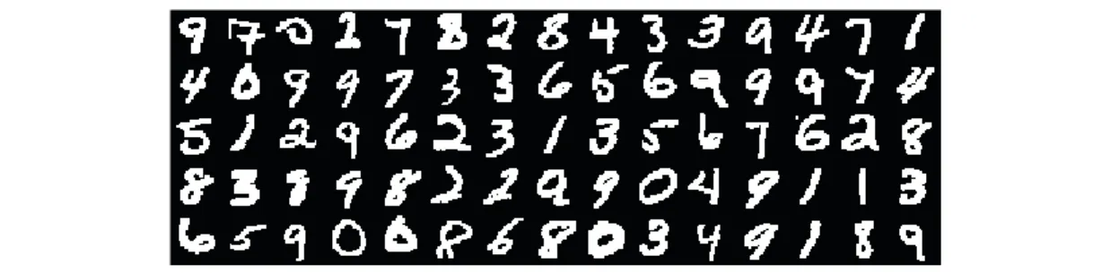
1.1 Examples of hand-written digits from the USPS dataset. The task is to recognize

the different digits and to separate all samples into ten classes. . . 2

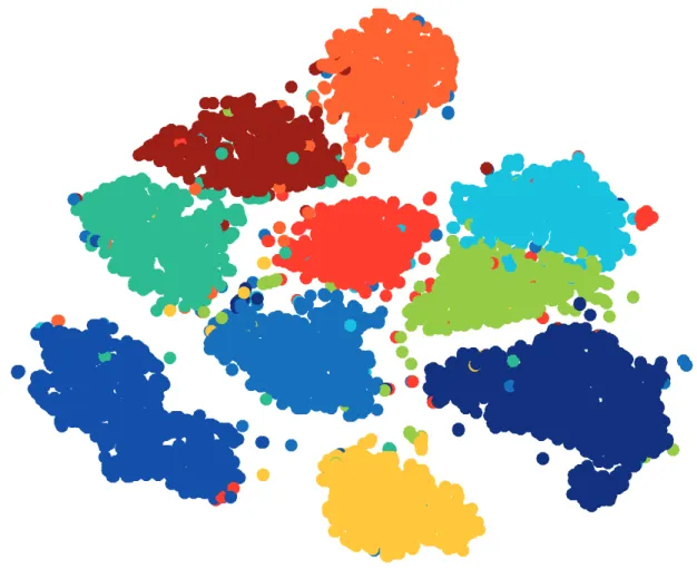
1.2 Clustering of the USPS dataset into ten classes. . . 3

1.3 Data acquisition with MNIST dataset. . . 4

2.1 An example graph signal representing traffic data in Minnesota. . . 14

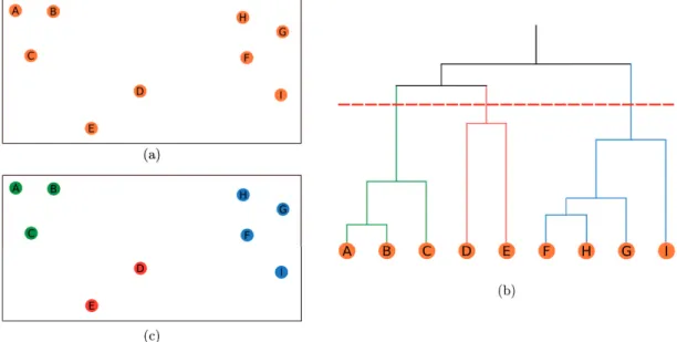
2.2 Dendrogram representation of a dataset. . . 25

2.3 Example of hierarchical clustering . . . 28

3.1 Study of the number of filtered signals on the assignment quality. . . 45

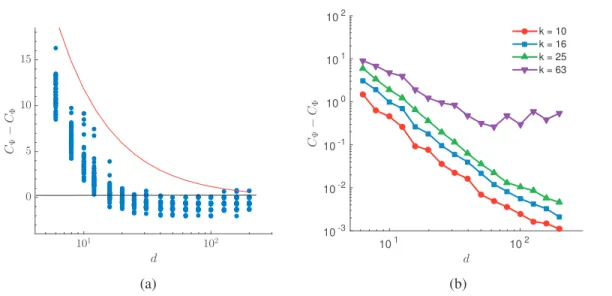
3.2 Accuracy of the theoretical bound of eq. (3.7) . . . 46

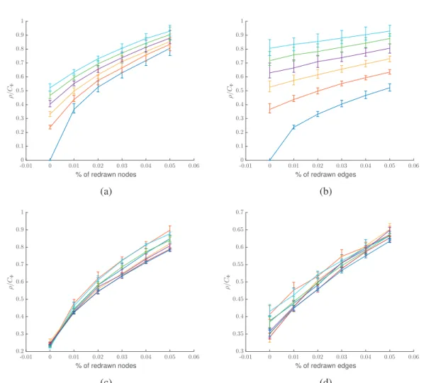
3.3 Impact onρof perturbation models for SBM . . . 54

3.4 Benefits of DynCSC over synthetically perturbed SBM. . . 56

3.5 Study of the proportion of filtered signals to reuse in dynamic graph clustering. . 56

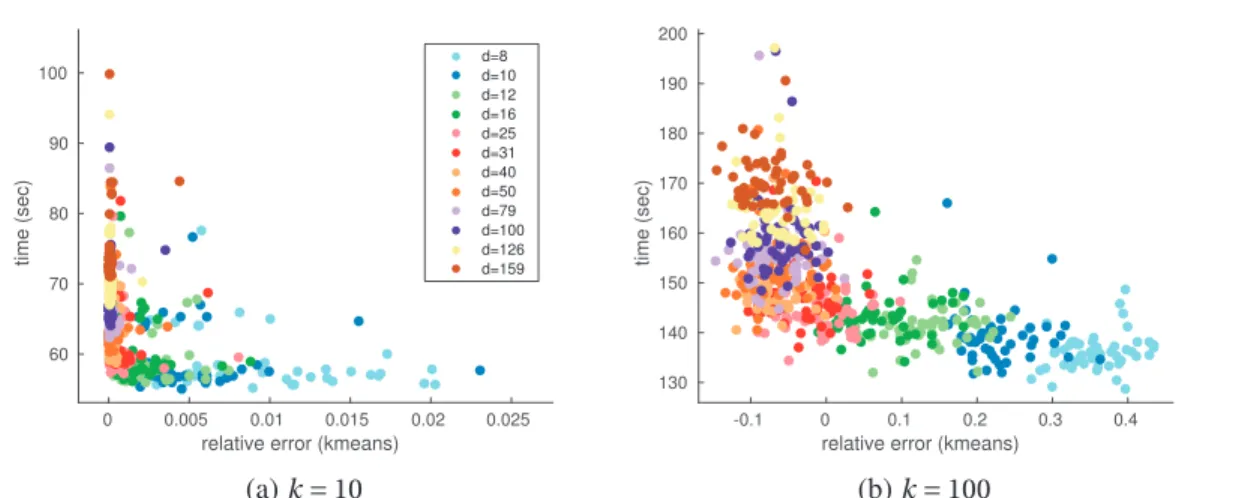
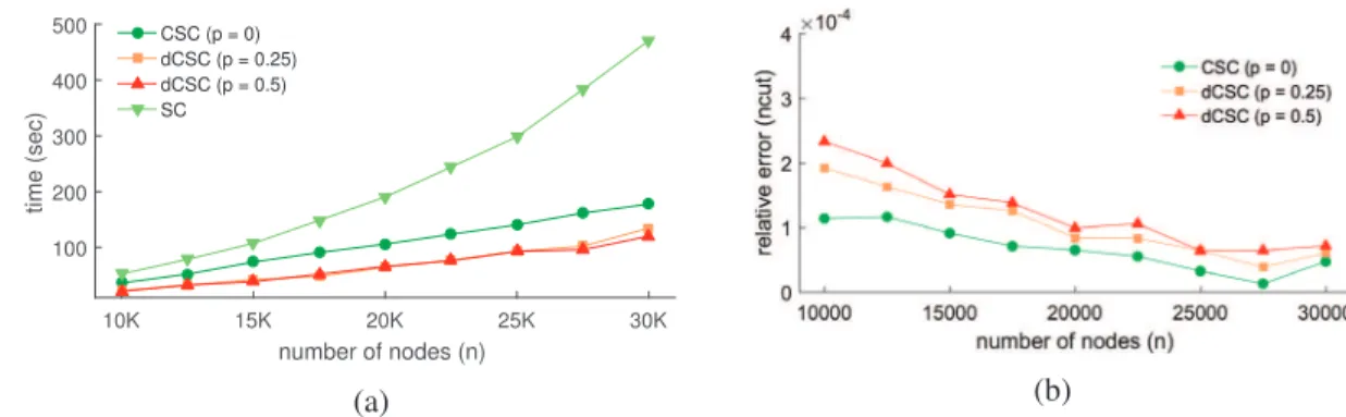
3.6 Scaling capabilities of SC and its approximations. . . 57

3.7 Statistics of our Arxiv dataset. . . 58

3.8 Comparison of DynCSC with SC and CSC on the evolutive graph of Arxiv citations between 1992 and 2004. . . 59

4.1 Quality of the second eigenvector estimation with FEARS. . . 69

4.2 The effect of approximating a step function with polynomials. . . 71

4.3 Timing of eigensubspace estimation. . . 78

4.4 FEARS applied to synthetic clustering of SBM. . . 80

4.5 2D projection of a Swissroll using FEARS. . . 83

4.6 Visualization of MNIST with FEARS and compared against state-of-the-art methods. . . 85

5.1 Information diffusion using heat kernel. . . 90

5.2 Approximation ofk-medoids with diffusion. . . 93

5.3 Approximation of the central nodes withTig 2 2. . . 94

5.4 Experimentation ofTig to determine the class centers with unbalanced classes. 96 5.5 Clustering quality of the light clustering method compared to Spectral Clustering on SBM of different clusterability. . . 100

List of Tables

3.1 Comparison of dynCSC against state-of-the-art methods. . . 58 4.1 Quality of the subspace approximation in theory and practice. . . 68 4.2 Measure of the approximation of the ideal low-pass filter with polynomial

ap-proximations. . . 70 4.3 Quality evaluation of our proposed methods for eigenspace estimation andλk

estimation . . . 74 4.4 Computational benefits of FEARS and compressedk-means in real world clustering. 81

4.5 Quality evaluation of FEARS and compressedk-means in real world clustering. . 81

4.6 Timing of 2D visualization of real-world datasets comparing FEARS with state-of-the-art methods. . . 84 5.1 Quality evaluation of the approximation ofk-medoids with kernel diffusion. . . . 92

5.2 Scaling capabilities of the light clustering method compared to Spectral Clustering.100 5.3 Comparison of light clustering with SC on the MNIST dataset clustering task. . . 101 5.4 Timing with the energy-based determination method for different graph kernels

and parameters. . . 101 5.5 Timing with the agglomerative selection method for different graph kernels and

parameters. . . 102 5.6 Quality evaluation using modularity with the energy-based determination method

for different graph kernels and parameters. . . 102 5.7 Quality evaluation using modularity with the agglomerative selection method for

different graph kernels and parameters. . . 102 5.8 Quality evaluation using the ncut objective with the energy-based determination

method for different graph kernels and parameters. . . 103 5.9 Quality evaluation using the ncut objective with the agglomerative selection

1

Introduction

Data is at the heart of the modern world. More or less every human activity relates to data. From purchase records, to social interactions, going through medical examinations, geo-positioning or internet browsing, our everyday activities generate tremendous amount of data. People use it to impact our daily life. For instance, purchase records might help target advertisements and suggesting interesting sales to the consumer, while aggregated medical records are expected to help understanding the causes of diseases. Even if the emergence of the internet in the last decades and, more recently, the global digitalization facilitated significantly the recording, storage and access to these pieces of information, data has been here since the very beginning.

Human beings have always been interested in preserving information from their past actions; experience is based on this previous knowledge accumulated over time. It is actually these very same data that allowed the understanding of our primitive History through the paintings of Lascau or the clay tablets found in Mesopotamia. However, while preserving information was reserved to a small number of people originally, it has been extremely facilitated in our modern world and one can now record and distribute any piece of information in real time across the world. This has dramatically lowered our expectations of the importance of stored data and led us to the generation of amazing volumes of data of partial interest. Indeed, studies show that 90% of the data that we now possess has been generated in the last two years. This means that 10 times more data should arrive in the next two years at that pace to reach an expected data volume exceeding 40 Zettabytes (4e22 bytes) in total by 2020. A significant part of it results

from the recent development of smartphones, Internet of Things (IoT) and wearables. These new sensors are of particular interest because they allow to measure events for which no systematic source of data existed so far. Interesting use cases include public transportation sensing [57, 22], personalized healthcare systems [28, 142] or optimizing the power grid [87] to cite a few. Moreover, with the new habit of storing everything, we noticed that all these tiny pieces of activity allowed to comprehend our world better. This trend made companies realize how important the data that they were producing could help them improve their services and profitability. With 80% of the information created and used by companies being unstructured, the necessity of data

analysis has never been as important.

A very famous, and quite old, example of classification problem is that of USPS (US postal service) who tried to recognize the digits on letters to automatically process the mail. They hand-labeled some of the instances of each of the ten categories (one category per digit) in order to illustrate the possible variations in the writing. Then, the goal was to classify all the incoming digits based on the knowledge base constructed with the hand-labeled samples. The initial database for the training contains 7’291 samples, which is already a lot to label by hand. However, in comparison with today’s volumes this is nothing. Statistical inference and learning thus became a large field of computer science; computational learning helping automatize various tasks.

Figure 1.1 – Examples of hand-written digits from the USPS dataset. The task is to recognize the different digits and to separate all samples into ten classes.

More recently, one of the major problems became the high speed of data. Due to the lack of interest for it in a near future, we want to compute a lot very fast or we will not need the output when it will be ready. Consider it in the following way: as a shop owner, it would be interesting to use the purchasing data of a given store accumulated over time to predict the attendance and help design the schedule for the months to come but this will not be of any help if the computation time is so large that the event that we want to predict happens before the predictions are produced. This imposes two important constraints in the design of new techniques: they must be able to manage very large datasets, on the one hand, and simultaneously, they must produce their results as quickly as possible. One must thus ensure that the complexity and the storage required to process the data are as low as possible. These two constraints are at the heart of this work and will be our primary focus when proposing new techniques for the analysis of data.

In most applications, hand-labeling is highly time consuming and expensive, even practically infeasible in some cases, because it requires expert knowledge, which is not always accessible. Thus, one of the tracks in automatized learning concerns only the unsupervised problems: those for which no ground truth is provided with the data. In this setup, one can expect to regroup similar data points and allow to efficiently characterize the incoming entries in the future. This is the goal ofdata clustering. For instance, assuming that USPS did not have the capability to hand label the digits in the mail, we could try to separate the different images into the ten categories based on their similarity.

Figure 1.2 – Clustering of the USPS dataset into ten classes.

The current situation points to a clear direction, that of improved data analysis techniques. More specifically, we focus in this thesis on the study of unsupervised methods and especially the task of data clustering. When applicable, we will extend the proposed method to the neighboring fields of data visualization and dimensionality reduction. In this context, the main question that I would like to contribute to in this thesis is the following:

What tools could we design to improve data clustering in order to reduce the computational time required to process the current volume of information? There are no doubts that a large number of researchers already addressed the problem of efficiency in data analysis. Indeed data science has already been a strong study field for a couple of decades. Actually, the methods used to extract efficiently meaningful pieces of information from the growing corpora at hand are split around several topics of interest, which are closely related. First isdata acquisition, which we could consider as data preprocessing. A piece of information such as an image can be acquired with various levels of details impacting its quality for instance

and also its size. When we try to understand a phenomenon based on a dataset, what is commonly done in the field is to extract the characteristics of each data point, that we callfeatures. Obviously, the more features we have, the more complicated will be the processing and thus the longer. We usually define thefeature spaceas the huge set of all the potential items that could exist. Sticking to the previous example with USPS data, we could characterize the images with their pixel colors generating a feature space of dimension proportional to the product of the width and the height of the image. On the extreme opposite, for instance under very tight space constraints, we could simply store the color of the average of the pixels and reduce the feature space to a one-dimensional space.

While this last example is an extreme case that has little practical purpose, we are interested in representing information with the smallest dimension that allows to solve the task. Very often, this will translate into a question of trade-offs between quality and speed. This is because the vast majority of embeddings that allow to reduce the dimensionality are discarding part of the information. This goes into a second category:dimensionality reduction.

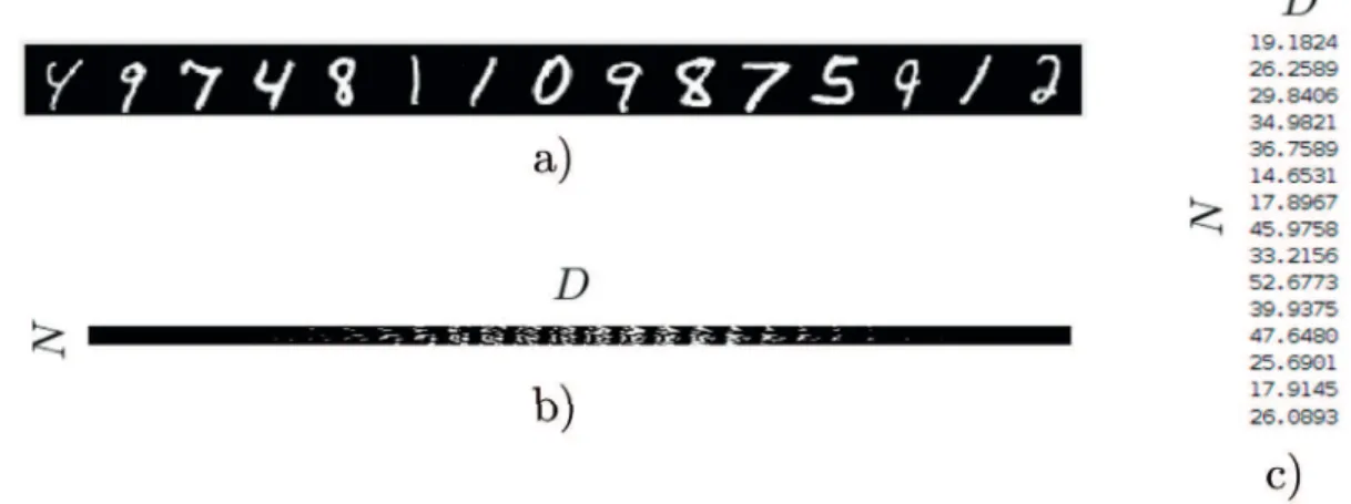
Figure 1.3 – Data acquisition of N =15 samples from the entries of MNIST under various representations. (a) displays the input data in the format it was scanned. (b) is the N×D

feature matrix associated with the entries above, where each column corresponds to a given pixel (D=784). In both (a) and (b) values are stored as integers in[0, 255]but are displayed in grayscale. (c) is an extreme application of dimension reduction where only the average of the pixels is kept andD₌1.

Ultimately, in order to visualize the data points one would reduce the dimensions down to two or three. Indeed, our comprehension of data also depends on our ability to represent it and get insights from it. Unfortunately, humans have difficulties to interpret data with many dimensions. Since we are not good for visualizing in more than three dimensions, a key challenge is to display the elements in such a space while they originally live in much larger spaces in order to simplify information while keeping the major differences on display. This specific reduction belongs to data visualization.

Overall, the field of dimensional reduction has been very active [134, 42] and at the same time the task of features selection has been clearly recognized through many research testing criteria to particular tasks [25, 117, 141]. Being able to accelerate even further the task of dimensionality reduction would help in the analysis of datasets, especially when the number of features is extremely large.

In the context of data clustering, a common practice of data preprocessing consists of constructing a graph from the high dimensionality features of the data points after their extraction. Graphs are useful because they allow to represent high dimensional objects with a single vertex and to model the similarity between the different entities with its links. They also contribute to the idea that the intrinsic dimensionality of a graph-based representation of a data set is actually lower than that produced by the feature extraction that we apply. Indeed, the construction of the graph would help capture only the intrinsic dimension, performing dimensionality reduction that would both fasten the following computations and help to explain the correlations between samples. Moreover, social networks and virtual interactions opened new perspectives to social sciences allowing studies to overpass the geographic limitations and ease the observation of masses. In these applications, graphs are natural ways to represent the data of study. In particular, we witnessed, in the last decades, the development of social networks like Facebook or Twitter but it goes much further in the scientific communities. Generally speaking, networks are interesting because they provide a well-structured information layer on top of data. We use them commonly to connect different pieces of information together and not specifically when it comes to people. Network science has also been very useful for gene expression, vehicular traffic monitoring, influence detection, epidemics localization and many more. In this thesis, the goal is to address methods that can be applied both on raw data as well as network data.

Motivations

In the past, many accurate techniques have been introduced to tackle the questions of dimen-sionality reduction, clustering, and visualization. Mostly, they used the fact shared among those problems that high-dimensional data (inRD) often admits an accurate low-dimensional intrinsic representation. Finding this embedding alleviates the processing and storage constraints of further processing tasks by representing data points in a space of smaller dimensionsd≪D.

In particular, it gave rise to the domain of low-rank representation and spectral graph theory that are theoretically well-founded and allow to solve the partitioning problem optimally. This enabled great improvements in the domain of data clustering and introduced the problem of graph eigendecomposition.

Eigendecomposition has been at the core of famous techniques used to extract low-dimensional embeddings from high-dimensional data by using the eigenvectors associated with specific eigenvalues. This has been used for partitioning (e.g., spectral clustering [98, 122]), data visualization (e.g., Laplacian eigenmaps [12]), but also simply as a dimensionality reduction

technique for preprocessing (e.g., principal components analysis [70]). The main drawback of all the aforementioned techniques is that they tend not to scale well as they have a rather high complexity. Indeed, a full eigendecomposition of the covariance matrix between feature costs O_D3.

The recent development of Graph Signal Processing (GSP) provides new tools for the study of diagonalizable matrices using frequency analysis, similarly to what is done in Discrete Signal Processing. The reader is referred to Chapter 2 for a detailed introduction. Within this framework, I will propose a set of new techniques for dimensionality reduction and clustering applied in particular to network data. I will briefly recall a way to extend these techniques to any data analysis problem by constructing graphs based on the data similarity, using nearest neighbor graphs.

With these tools, I suggest taking a new look at spectral graph theory. We are now capable of avoiding the computation of the eigendecomposition while still obtaining the well-studied solution of partitioning. This allows to reduce drastically the complexity of the quite old method of Spectral Clustering (SC) with a loss of accuracy that is both small and adaptive to the task. One can indeed decide to set the threshold between speed and accuracy at her will. This new approach sets a whole new viewpoint and promises to go even further.

Well designed filters of a given kind will allow to solve the eigendecomposition problem while others tend to provide graph centrality measures efficiently. With the latter, I aim to replace the

k-means algorithm, very often used for data partitioning and underlying in a lot of algorithms

across various domains. Overall, the goal with GSP is definitely to help solve some of the central problems of data science, not necessarily with an improved accuracy but providing ways to apply them efficiently on large amount of data while achieving an accuracy similar to some of the most famous algorithms existing so far.

Contributions and thesis structure

I describe in more details the state-of-the-art inChapter 2, together with the basic definitions

and the notation used throughout this thesis. It contains an introduction to GSP, presenting the fundamental results on which the rest of the thesis is built. This chapter also serves to describe comparative methods in detail in order to present the benefits of the following works.

This thesis then focuses on the improvement of approximated methods mainly for the task of graph clustering using the latest developments in the field of GSP. In this regard, inChapter 3, I

recall the recent advances based on filtering of random signals and propose two improvements. On the one hand, I analyze theoretically the assignment quality guaranteed by the random filtering and establish a characterization of the approximation error to SC and a way to trade between accuracy and time. On the other hand, I introduce a natural extension for dynamic graphs where I consider that connections between the entities can vary over time and thus impact the partitioning

of the graph. We will see that one can reuse part of the information from the previous time step in order to approximate the result of SC with a reduced complexity.

Clustering, visualization and dimensionality reductions have an important common factor that is also studied in this thesis inChapter 4. By contributing to the problem of efficient graph Fourier basis determination, we will see that we can improve the complexity for exact subspace recovery and thus the problems that use it such as visualization (with Laplacian eigenmaps) or graph clustering (with spectral clustering). Although not perfect for Principal Component Analysis (PCA), I show how to use this for Principal Component Projection (PCP).

Then, since graph clustering is at the heart of this thesis, we will also see how the localization operator defined on graphs can help partitioning graphs inChapter 5. I will briefly talk about

structural clustering where nodes are grouped based on their role in the graph, and not their similarity anymore before I move to use this tool for standard clustering. Since I present how to avoid the eigendecomposition in SC in the previous chapters, I now try to remove thek-means

step using properties of graph signals.

Finally, Chapter 6summarizes the findings and concludes the work. It also presents future

directions that are left as open problems and would benefit from additional research. A natural extension to this problem would be to consider multilayer clustering next. The primary concern is to combine several sources of information to cluster a single set of nodes. This problem is very interesting because we often possess several sources of information that we do not know how to combine and end up combining them to obtain a single adjacency matrix.

In the various chapters of this thesis, all the experiments are designed using the open-source Graph Signal Processing toolbox (GSPBox [107]) and the code is available on my personal Github account to promote open research and collaborations: https://github.com/lionel-martin/. Please note that since our methods use random processes, it is expected for the results to be slightly different in the details, but overall consistent with the presented figures and tables.

2

From Signal Processing to Clustering

This chapter will present the foundations of the works presented in the following of the thesis. It regroups all the pre-existing tools and techniques that are of principal interest for one or several of the following chapters together with the most famous and/or best performing methods of clustering with which this work should be compared.

It is organized into a couple of distinct parts. The first one is dedicated to the study of signal processing on graphs, starting from the formal definition of graphs to the latest development in the signal processing field around it. The second part is specifically going to present various data analytics methods and connects data clustering to graph clustering, our primary focus. Finally, a presentation of very famous clustering techniques, used in the latter parts as baselines for the evaluation of the quality of our proposed methods, gives a good opportunity to recall the mathematical properties behind it.

Notation

All along this thesis, we will use a consistent notation regarding the variable names. • Sets are written with calligraphic letters (e.g.,A,B) as well as the usualN,ZandR; • Scalars are denoted with lowercase letters such asaorb;

• Vectors are defined as column vectors and are represented with boldface letters (e.g.,a,b);

• Matrices and higher order tensors are bold uppercase letters (e.g.,A,B). Their elements are

referred to using comma-separated indices such asAi,j for a matrix, defining the element

in thei-th row andj-th column;

• Functions defined over matrices have to be interpreted as elementwise operations over diagonal matrices. For non-diagonal matrices, we should first diagonalize it and then apply the elementwise operator. For instance, ifgis a univariate variable overR,g(L)₌Ug(Λ)U⊤

2.1

Fundamentals of Graph Signal Processing

2.1.1 Graph theory

Graph theory is a field of discrete mathematics, whose origin dates back to several centuries ago, that is dedicated to the concept ofgraphs. Graphs are mathematical structures, generally used to model connections between two different entities. Although graph theory was initially used to solve puzzles such as the seven bridges of Königsberg [44] or the Knight tour problem [110], graphs’ discrete structure made it a compelling field. Over the centuries, lots of theories involving graphs were proposed and various problems were solved such as perfect matching, coloring, routing, covering and more [18]. It thus became the ideal tool to observe networks in the recent developments of network science, given its core properties making it both a good data structure for the problems posed on networks and a well-studied tool for routing problems. Graphs are at the center of the works presented in this thesis. We will start this section by an introduction of graphs and add concepts related to these objects in a step by step fashion. We define a graphG by a triplet(V,E,W)whereV is the set of vertices (also called nodes throughout

the thesis with no distinction) andEthe set of edges representing connections between nodes in V. AdditionallyWweights the different edges, characterizing how the nodes relate to each other.

The verticesv_∈V of the graph are ordered fromv1tovN,N= |V|. In the most common setting,

an edge is a direct connection between two nodes of the graph:E_⊂V_×V. Rarely, we will be

considering hypergraphs instead that are constructed in the same way except edges will become abstractions connecting a subset of the nodes together: E _⊂P(V), the power set of V. We

characterize the graphs depending on the number of edgesM_{= |}E_|. We callsparse graphsthose withM=O_(N)and_{dense graphs}when_M=Θ_(N2₎. In between, the characterization is not well defined.

The matrixWis called the weighted adjacency matrix of the graphG. This can be interpreted

as a similarity measure between the nodes and is the most important part of the description of the graph. Although this might be an oversimplification in practice sometimes, a common assumption that we will also make throughout the thesis is that the connections are symmetrical, that is, the connection froma tobis as important as that fromb toa. Such graphs are called

undirected graphs.

The elementWi,j represents the weight of the edge between verticesvi andvj and a value of 0

means that the two vertices are not connected. The degreedi of a nodevi is defined as the sum

of the weights of all its edges

di= N

j=1

Wi,j. (2.1)

2.1. Fundamentals of Graph Signal Processing

Another characterization of the graph connectivity is represented through the incidence matrix of the graph, which we will be using in the following of this chapter.

Definition 2.1: Oriented Incidence Matrix.

The oriented incidence matrixE of a graph is a matrix of size|V_{| × |}E_|where each column

describes an edge. In weighted directed graphs, the elements are populated with values such that:

Ei,j=          −Wi,j, ifei,j leavesvi Wi,j, ifei,j entersvi 0 otherwise (2.2)

The undirected case is treated similarly by selecting any extremity of each edge as the source, setting the remaining as sinks.

Through this thesis we will be referring to a small set of different synthetic graphs, useful to give insights on the new techniques that we will present. In the following, we present the properties of these various graphs.

Example 2.2: Nearest Neighbors Graph.

A Nearest Neighbors Graph (usually called NN-graph) is a graph whose edges are defined based on a distance metric between the vertices and where only the closest ones are connected to each other. Nodes are usually positioned beforehand into a dimensional space depending on their features. Often, the distance metric is defined to measure their similarity, usually as a kernelized version of the Euclidean norm (ℓ2-norm):d(u,v)=kfu−fv

₂.

There are two common classes of unweighted nearest neighbors. One is based on the number of neighbors, calledk-NN graphs it restricts the connections to thekclosest vertices of each source.

The other one is namedǫ-NN graph and keeps only the neighbors at a distance of at mostǫof their source independently of the number of close neighbors.

Additionally, the weights of the edges can either be binary (i.e., 1 when there is a connection and 0 otherwise) or be a function of the distance between the two vertices. We refer the latter model as the kernelized NN-graphs. Among the different kernels, the Gaussian kernel is prominently used and yields the following weighting

Wi,j=exp −d(xi,xj) 2 σ2 , (2.3)

whered(·,·) is the distance metric of your choice andσ describes the speed of decay of the exponential. When not specified, we will be using the Euclidean distance fordand the average

Example 2.3: Sensor Graph.

A sensor graph is ak-NN graph whose nodes have been randomly placed in the unit square inR2. It resembles networks of measurements such as temperature networks or traffic networks, hence the name.

Example 2.4: Stochastic Block Model.

The Stochastic Block Model (SBM) is a probabilistic generative model of graphs designed specifically for clustering tasks. In this model, all the nodes are assigned a class between 1 and

k at the beginning. Then, the graph is populated based on the class appertaining of the two

extremities of the edge. Namely, if two nodes u andv belong to the same class, they have a

probabilityq1of being connected. On the opposite, if they do not have the same class, the edge

probability isq2. We refer toq1 as the intra-class probability while we callq2the inter-class

probability. By definition, we must setq1>q2 in order to emphasize the clusterability of the

graph.

Abbe et al. [1] studied the regimes where we could almost surely detect a community structure. They deduced that ifq1,q2∝log(_NN)and q1+₂q2−q1q2>log(_NN) then such community structure

existed.

Alternatively, this model can be characterized entirely with the knowledge of the average degree in the graphdG and the ratioε=q_q2₁. Decelle et al. [36] suggested the existence of a threshold

above which community detection is impossible:

εmax= dG− dG dG+k−1dG . (2.4)

For a given ratioε,q1andq2can be determined assuming that the sizes of the classes are known.

If we call themni fori=1, . . . ,kwe have q1=

dGN

k

i₌1ni(ni−1+ε(N−ni))

and q2=q1ε. (2.5)

If we assume thekclasses to be of equal size, this yields q1=

dGk

N(k₋1)ε₊N₋k and q2=q1ε. (2.6)

Example 2.5: Erdös-Rényi.

Named after the two scientists that made a breakthrough in the field of random graph theory [43], this model is a simplified version of the SBM. Here, no classes are assigned beforehand and all edges have the same probabilityp.

Additionally, the authors proved that if p> (1+ε) ln(N N), then the graph will be almost surely

2.1. Fundamentals of Graph Signal Processing

We decided to make two remarks before we proceed. First, this model is important in graph clustering because it sometimes serves as the null hypothesis for clustering. Indeed, given its construction, it represents a set of graphs that do not possess any community structure. Then, the study of the discrepancies between a graph of interest and the statistics of the Erdös-Rényi points out the potential community structure of the given graph. This topic is detailed in Sec. 2.2.4. Second, note that we can also reuse the property of connectivity to compute the threshold for

q1andq2in the SBM to ensure connectivity. By computing the average probability in an SBM,

assuming uniformly distributed clusters, this gives

dG N = q1+(k−1)q2 k > (1+ε) ln(N) N . (2.7) 2.1.2 Graph signals

When the nodes of the graph represent locations (e.g., with sensor graphs or road networks), additional data is associated with the nodes. The reader is referred to Fig. 2.1 for an example of traffic data where the nodes are crossroads that possess the additional information of the jam at their position. The fluidity of traffic is a signal living on the graph. In practice, it frequently happens that the graph generated from a dataset represents the sampling of a continuous structure that might be known or not. In such a case, the assumption that the data is smoothly evolving on the graph is often used to model the behavior of the phenomenon under study. This can be measured by summing the square of the differences between each pair of connected nodes and this measure corresponds to the Dirichlet energy of the process. However, the signal can also be simply a categorization of the different parts of the network (e.g., for the study of epidemics or influence detection). We now introduce the mathematical definition of graph signals before to go back to Dirichlet energy and smoothness.

Definition 2.6: Graph signal.

A graph signalf is defined as an application f :V _→Rand is represented as a vector of sizeN

where thei-th component of the vector is the value of the signal at vertexvi. Multidimensional

signals can be defined by extension as a vector of value instead of scalars on the nodes, potentially describing temporally evolving behaviors.

From there, an important mathematical tool that has been defined is the Laplacian. There exist several definitions possessing each a slightly different interpretation but all of these relate to the continuous definition of the Laplace operator on Euclidean spaces, hence the name.

The link between the two has been presented in great details in [13] where they highlight the fact that it can be expressed as the divergence of the gradient over graphs. In this case the gradient

(a) Map data ©2017 Google (b) Minnesota graph with traffic signal

Figure 2.1 – An example graph signal representing traffic data in Minnesota.

computes the derivative along all the edges of the graph based on the value at its endpoints ∇Gf e=(vi,vj)= _∂f ∂e e=(vi,vj)= Wi,jf[j]−f[i] (2.8)

and the divergence is its adjoint operator.

The gradient in this case can be represented by a multiplication with the incidence matrix of the graph. Indeed, we have

E⊤f e= Wi,jf[j]−f[i] =∇Gf e₌(vi,vj) . (2.9)

With this definition, the Dirichlet energy that was discussed above can be computed as

f⊤EE⊤f _=∇Gf ⊤ ∇Gf = e=(vi,vj) Wi,j(fi−fj)2. (2.10)

This provides the most common definition of Graph Laplacian which is that of the combinatorial LaplacianLC simply computed as

LC=EE⊤=D−W. (2.11)

While possessing already useful properties for the analysis of the graph structure, there exist two additional famous versions of the Laplacian that we are going to present quickly before explaining with more details its properties.

2.1. Fundamentals of Graph Signal Processing

components in order to be unaffected by the local node degree. Its formulation is

L=D−12L_CD− 1

2. (2.12)

The second one is the random walk Laplacian:

LRW=D−1LC. (2.13)

This one contains in its elements the probability distribution of the random walk over the graph following the edge weight as prior for the next movement.

In the last two cases, by convention, we setD−

1 2

i,i =0whendi=0and thusLi,i=0for isolated

verticesvi. For graphs with no isolated vertices, we can relate the Laplacians to the weight matrix

as:

L=I−D−12_WD− 1

2 and _LRW=I−D−1_W. (2.14)

2.1.3 Spectral theory

Now that signals are defined, signal processing is a natural way to proceed for its analysis. In traditional signal processing, signals represent the amplitude of temporal observations of an event (either continuous or discrete). Among the different transforms, the frequency content can be obtained via a Fourier transform of the signal. Frequency analysis allows to perform lots of different operations on the signal in order to improve it (e.g., denoising) or to ease its transmission or storage (e.g., compression) for instance.

The signals defined on graphs cannot be interpreted in the Fourier domain following the traditional signal processing workflow. However, we would like an operator that would allow its frequency analysis. Noticing that in the time domain, the classical Fourier transforms compute the inner product of the signal with the eigenfunctions of the Laplace operator, a natural definition for the Graph Fourier Transform (GFT) is to take the inner product with the eigenvectors of the graph Laplacian. To this end, we first need to define the eigen-decomposition of the Laplacian.

Definition 2.7: Eigendecomposition of the Laplacian.

By application of the spectral theorem, we know thatLcan be decomposed into an orthonormal

basis of eigenvectors noted uℓ_{ℓ=0,...,N−1}. The ordering of the eigenvectors is given by the

eigenvalues notedλℓ_{ℓ=0,...,N−1}sorted in ascending orderλ0≤λ1≤. . .≤λN₋1=λmax.

The eigenvalues are computed by minimizing the following objective λℓ= min

f∉Sℓ−1 f⊤Lf

f⊤_f , (2.15)

of the minimizer of each eigenvalueλℓis theℓ-th eigenvector associated with this eigenvalueuℓ.

In a matrix form we can write this decomposition as L₌UΛU∗ withU₌u0

. . .uN₋1the

matrix of eigenvectors andΛthe diagonal matrix containing the eigenvalues in ascending order.

It is called a Fourier transform by analogy to the continuous Laplacian whose spectral components are Fourier modes, and the matrixUis sometimes referred to as the graph Fourier matrix (see

e.g., [33]). By the same analogy, the setλℓ

ℓ=0,...,N−1 is often seen as the set of graph

frequencies [126].

We now have the tools to represent the Fourier transform on graphs.

Definition 2.8: Graph Fourier Transform.

Given a signal f defined over the vertices of a graphG, its GFTfis defined by the inner product

of f with the eigenvectors ofL. We thus have

f[ℓ]_{= 〈}f,uℓ〉 = N

i₌1

u∗_ℓ[i]f[i] or equivalently in matrix form f=U∗f. (2.16) SinceUis an orthonormal basis, the inverse Fourier transform is simply

f =Uf which corresponds to f[n]= N−1

ℓ=0

uℓ[n]f[ℓ]. (2.17)

The Laplacian1_{is an interesting operator for graphs since it combines a complete characterization}

of the graph and useful algebraic properties. We will conclude this section by presenting some of them and refer interested readers to [33, Chap. 1] for a deeper analysis.

Properties 2.9: Graph Laplacian.

First, we present several properties that work for both the combinatorial and the normalized Laplacians. A very simple fact about those two is that they are symmetric matrices. Thus, the eigenvalues of their eigen-decomposition are all real and non-negative. On top of that, they both possess 0 as an eigenvalue. Indeed, if we take u0= 1_N, then LCu0=0 and similarly

with f ₌D12u₀ for the normalized Laplacian L_N. Actually, this particular eigenvalue has a

multiplicity that depends on the connectivity of the graph. Indeed, for a disconnected graph with

c components of sizesN1, . . . ,Nc, thecsignals containing the constant value _N1_i for the nodes

of thei-th component and zeros elsewhere all returnLCf =0hence producingcorthonormal

signals that are thecfirst eigenvectors of the graph Laplacian.

Next, note that the normalized Laplacian has a bounded spectrum, withλmax≤2. This is an

equality if and only if the graph is bipartite, meaning that the graph can be separated into two

1_{We interchangeably mean the Laplacian matrix, and the operator defined by the multiplication of the Laplacian} in the rest of the thesis.

2.1. Fundamentals of Graph Signal Processing

disjoint subsetsSandS¯and the edges all possess one end inSand the other one inS¯. Regarding

the spectrum of the normalized Laplacian, we also know that

ℓ

λℓ≤N, (2.18)

with equality if and only if the graph does not possess isolated vertices (vertices with degree 0). More generally, sinceTr(LN)=Tr(Λ), the sum of the eigenvalues corresponds to the number of

non-isolated nodes in the graph.

2.1.4 Filtering graph signals

The frequency analysis of graph signals called for the definition of operations defined in the frequency domain. Continuing on the example of smooth signals on a discretized surface, we notice by definition that those must possess only low-frequency components in order to possess low Dirichlet energy. Thus, filtering out the high frequency components of a signal can help to generate smooth signals on a graph. It can also serve to compress complex signals into smooth approximations defined by only a few components.

One of the most important properties of Fourier in the traditional domain is that convolutions in the time domain are transformed into multiplications in the frequency domain. This property is preserved in graph analysis as we recall in the next definition.

Definition 2.10: Graph convolution.

Let us denote the GFT of a given signalxwithx=F{x}. If we now consider two given signalsx

andy, the convolution between the two signals reads

F x∗y[ℓ]₌x[ℓ]_·y[ℓ] thus x∗y[n]=F−1x·y[n]. (2.19) Thus, filtering can be carried out by a pointwise multiplication in Fourier in the exact same way as in the traditional domain. To this end, we define a graph filter as a continuous functiong:R+→R

directly in the graph Fourier domain.

Definition 2.11: Graph filtering.

If we consider the filtering of a signal f, whose GFT is written f, by a filtergthe operation in the

spectral domain is a simple multiplication f′_{[ℓ]=g(λℓ)·f[ℓ], with f}′_andf′_{the filtered signal}

and its GFT respectively. Using the graph Fourier matrix to recover the vertex-based signals, we get the explicit matrix formulation for graph filtering:

f′=F−1g(λℓ)·f[ℓ]=F−1g(Λ)F f. (2.20)

vector-matrix formulation for the graph filtering:

f′=Ug(Λ)U∗f. (2.21)

Using the definition of functions over matrices,g(L) :₌Ug(Λ)U∗_{, this is most often shortened}

into

f′₌g(L)f. (2.22)

Since the filtering equation defined above involves the knowledge of the full set of eigenvectors

U, it implies the diagonalization of the LaplacianLwhich can become intractable for large graphs.

To circumvent this problem, a solution is to determine the value ofg(L)without the knowledge of

U, bypassing the computation of (2.21). A common method, introduced in [58], suggests to use

the degree-nChebyshev interpolation formula. The authors noticed that the recurrence relation

used in the definition of the Chebyshev polynomials of the first kind allows to compute a faithful approximation of the filter iteratively and with a reduced cost.

Definition 2.12: First-kind Chebyshev polynomials.

The Chebyshev polynomials of the first-kind are defined with the recurrence relation

T0(x)=1 T1(x)=x Tn(x)=2xTn−1(x)−Tn−2(x). (2.23) Properties 2.13.

Among the different properties of the Chebyshev polynomials, we stress the fact that 1. Tn(x)=cos(narccos(x)),∀x∈[−1, 1]

2. The roots of the polynomial are xj ₌cosπ₂₍2_nj+₊1₁₎,j ₌0, . . . ,n. They are called the

Chebyshev nodes and are often used in polynomial interpolation since they minimize the Runge’s phenomenon (i.e., the fact that interpolation might increase the error with the polynomial order). Interpolating at these points provides an approximation close to the optimal solution under the maximum norm.

Definition 2.14: First-kind Chebyshev interpolation.

Given a continuous functiong: [−1, 1]→R, the degree-nChebyshev interpolation is gn(x) := n m=0 cmTm(x), wherecm= 2−δ(m) n+1 n j₌0 g(xj)Tk(xj). (2.24)

In our case, since the spectrum is not contained in[₋1, 1], there is an extra step of renormalization of the domain. The mappingθ:x→ λmaxx

2.1. Fundamentals of Graph Signal Processing

contained in the support. Finally, the Chebyshev approximation of orderPo of the graph filter is g(L)f _≈ Po m₌0 cmTm(L)f, wherecm= 2₋δ(m) Po+1 Po j=0 g(θ−1(xj))Tk(xj), andT0(L)f =f T1(L)f =θ(L)f Tm(L)f =2θ(L)Tm₋1(L)f −Tm₋2(L)f. (2.25)

Apart from this frequently used approximation, recent works in the GSP community also used Lanczos method to approximate any filter [129] and Jackson-Chebyshev approximation alleviat-ing the Gibbs oscillations of the standard Chebyshev approximation developed above [39]. In the particular case of approximating the sign function in[₋1, 1], Allen-Zhu and Li [6] proposed an approximationgn that converges even faster to the step function. It has been introduced jointly

with mathematical guarantees that we recall quickly.

Properties 2.15: Estimation of the sign function with truncated polynomials.

The approximation of the sign function with these polynomial can be as precise as necessary. The polynomial is guaranteed to:

1. _|gn−sgn(x)| ≤ǫfor allx∈[−1,−α]∪[α, 1],

2. gn(x)∈[−1, 0]for allx∈[−α, 0]andgn(x)∈[0, 1]for allx∈[0,α].

The choice ofǫandαenforce a minimum degree such thatPo_≥1

2αlog

3 ǫα2

.

This polynomial is constructed in two steps. First using Chebyshev approximation, we can generate a polynomial approximationqPo=

1₊κ₋x 2

−12 for_κ

∈[0, 1). Thengnis computed simply

asgn=x·qPo(1+κ−2x

2_{). The value ofκhas a direct impact on the approximation sinceκ} =2α2. Finally, the degree ofgnis2Po+1due to the composition ofx2andqPo(x).

All these methods scale with the number of edgesM and reduce the complexity of a filtering

operation to O_(PoM), which is especially advantageous in the case of sparse graphs. When the graphs are large, then Po _≪N and there is an undoubted gain to consider polynomial

approximations instead of theO_N3computational cost induced by the eigendecomposition.

2.1.5 Localization operator

The localization of signals over their support is interesting in general. For discrete time signals, which are defined over a chain graph, translations, corresponding to time shifts, enable the localization of the signal. Translations are, moreover, particularly useful for stationarity analysis. Here, the support (i.e., the vertex set) is not ordered and a direct transposition of the concept to graphs is an ill-posed problem. However, in contrast to discrete time signals, all frequencies are not spread equally over the nodes (while it is the case with time in signal processing). In fact,

frequencies can be localized around certain nodes depending on the graph and the generalization of localization on graphs can be organized around this fact.

Several attempts were made to generalize the concept of localization from time signals to graph signals . However, the lack of order over the support alters the meaning of a signal translation and requires to find a correspondence in the spectral domain instead. Shuman et al. [126] as well as Perraudin et al. [106] proposed similar definitions for the graph translation. They started from the classical definition of the translation being the convolution between a signal and a Kronecker delta in time. Using (2.19) they obtain similar definitions, up to a normalization factorN,

which we state in the following definition.

Definition 2.16: Graph translation.

Given a signal f _∈RN and a graphG, the translation on graph reads

Tif[n]₌

N−1 ℓ=0

f[ℓ]uℓ[i]uℓ[n]. (2.26)

Note that this definition of translation is very close to the definition of the Graph Wavelet Transform [58]. Moreover, we notice that this operator is kernelized and although any signal cannot be localized around a predetermined vertex, it is the case for filters defined in the spectral domain under certain assumptions. Since localization is an interesting property, that we will be using in the following chapters, we extend the definition of graph translation and callTig the

localization operator of the filtergaround vertexi:

Tig[n]= N₋1 ℓ₌0

g(λℓ)uℓ[i]uℓ[n]. (2.27)

An isometric alternative to the definition of graph translation has been proposed in [50] but this one does not possess the localization properties of filters.

2.1.6 Other approaches to GSP

The field of signal processing on graphs emerged simultaneously from different research groups in the recent years. Although, a large community agreed on the definitions stated above, there is an alternative concept called DSPG, mainly used by Moura and its co-authors [119, 88, 29], that

deserves to be quickly introduced as well.

The alternative approach, just as the one presented above, tries to extend the concepts of traditional signal processing to graphs. Similarly to the works on Graph Signal Processing, they also presented the ring graph (a cycle graph) as a convenient structure on which to start the comparisons but aim at defining different properties with this structure. Their corner stone is the definition of the equivalent of a time delay, denoted byz−1_{in the classical domain. For this specific application,}

2.2. Clustering

they define the graph shift as the shift of the signal on the vertices. Namelys˜[n]=s[n−1]with a circulant application on the borders of the domain ensuring thats˜[1]=s[N]. They generalize this with the notations˜₌AswhereAis the adjacency matrix of any graphG.

From that point on, they are able to characterize the class of linear shift-invariant graph filters and prove that it corresponds to the polynomials inA:H₌h0I+h1A+ ··· +hLAL. The form of

A being more general than that ofL, there is no guarantee forAto be diagonalizable and thus the

spectral decomposition associated withA isVJV−1, its Jordan Normal Form (JNF). For detailed

explanations about its determination, readers are referred to [138]. In practice, however, this decomposition is untractable because the form is unstable (e.g., aε-difference on the input can produce a very different output).

Although the application might not seem as obvious as spectral clustering in the case of GSP, the methods detailed in the following section could be extended to this definition of signal processing on graphs allowing potentially the computation of fast JNF. Despite the numerous applications that have been proposed following the two different approaches, the lack of complexity analysis in the DSPGcommunity makes it difficult to summarize the generalization in this section. We

refer the reader to the works on denoising [123, 29], stationarity [106, 88] and big data analysis [78, 120] for a deeper analysis of the frameworks allowing a clearer comparison between them.

2.2

Clustering

Clustering is an important problem in Artificial Intelligence (AI) that has long been studied and tries to solve the following problem: based on data, the goal is to find a categorization of the entries that assign together those with common properties and separate the dissimilar data points. It differs from classification in the sense that a ground truth is not required in order to classify the data points. This is advantageous because it avoids the need of experts attributing labels on the samples (or a subset of them) which can be very expensive and time consuming. Data processing is then easier to automatize.

The fact that many methods are proposed in the literature can be explained by a lack of rigorous problem definition. Many techniques share similar approaches but have different formulations. In particular, the definition of similarity, and thus the solution to the problem often depends on the application and the subjectivity of the criteria involved. Nevertheless, clustering is a famous field of research among the AI community, attracting even more interest than before with the data deluge. Famous works of clustering allowed the segmentation of pixels in images [122], objects recognition [79], information retrieval [68, 27], text recognition [26], data mining [14, 2], protein-protein interactions [143] and others. The basics and main contributions are highlighted in this section. For a deeper analysis of this large field, readers are referred to the surveys of Jain et al. [67], Fortunato [45] and Porter et al. [111] as well as the book of Gan et al. [47].