RIT Scholar Works
RIT Scholar Works
Theses11-14-2019
Deepfake detection and low-resource language speech
Deepfake detection and low-resource language speech
recognition using deep learning
recognition using deep learning
Bao Thai [email protected]
Follow this and additional works at: https://scholarworks.rit.edu/theses Recommended Citation
Recommended Citation
Thai, Bao, "Deepfake detection and low-resource language speech recognition using deep learning" (2019). Thesis. Rochester Institute of Technology. Accessed from
This Thesis is brought to you for free and open access by RIT Scholar Works. It has been accepted for inclusion in Theses by an authorized administrator of RIT Scholar Works. For more information, please contact
low-resource language speech
recogntion using deep learning
by
Bao Thai
A Thesis Submitted in Partial Fulfillment of the Requirements for the
Degree of Master of Science in Computer Engineering
Department of Computer Engineering
Kate Gleason College of Engineering
Rochester Institute of Technology
Rochester, NY
Approved By:
Dr. Raymond Ptucha Date
Primary Advisor - R.I.T Dept. of Computer Engineering
Dr. Alex Loui Date
Secondary Advisor - R.I.T Dept. of Computer Engineering
Dr. Emily Prud’hommeaux Date
ACKNOWLEDGEMENTS
I would like to take this opportunity to thank Dr. Ray Ptucha and Dr. Emily Prud’hommeaux for the guidance and continuous support in my research. I am also thankful for Dr. Alex Loui for being on the thesis committee. I would also like to thank Dr. Wright for the guid-ance on the audio spoofing research. I would like to thank Robert Jimmerson and Dominic Arcoraci for their help with the research on speech recognition for Seneca. Finally, I would like to thank all the friends and family for their support throughout my time at RIT.
Contents
1 Abstract 11
2 Introduction 12
2.1 Low-resource automatic speech recognition . . . 12
2.2 Audio spoofing detection . . . 12
2.3 Contributions . . . 13
3 Background 14 3.1 Acoustic modelling . . . 14
3.2 Mel-frequency cepstrum coefficients (MFCCs) . . . 16
3.3 Connectionist Temporal Classification (CTC) . . . 18
3.4 Language modelling . . . 20
3.5 Generative Adversarial Networks (GANs) . . . 20
3.6 Recurrent Neural Network (RNN) and Long-Short Term Memory cells (LSTM) 22 3.7 DeepSpeech . . . 25
3.8 Audio Spoofing . . . 26
3.9 Constant Q Cepstral Coefficients (CQCC) . . . 27
4 Previous works 28 4.1 Resource Constrained ASR . . . 28
4.2 Audio spoofing detection . . . 32
5 Datasets 33 5.1 Resource Constrained ASR . . . 33
5.1.1 Seneca dataset . . . 33
5.1.2 Iban dataset . . . 34
5.2 Audio Spoofing . . . 35
6 Methodology 36
6.1 Resource Constrained ASR . . . 36
6.1.1 Data augmentation . . . 36
6.1.2 Acoustic modelling . . . 39
6.1.3 Multi-staged learning . . . 44
6.2 Audio Spoofing . . . 46
6.2.1 Convolution-Recurrent Neural Network . . . 46
6.2.2 Convolutional-based detection . . . 47
7 Evaluation metrics 48 7.1 Low-resource ASR . . . 48
7.1.1 Character/Word Error Rate . . . 48
7.2 Audio spoofing detection . . . 49
7.2.1 Equal Error Rate (EER) . . . 49
7.2.2 Tandem Detection Cost Function (t-DCF) . . . 49
8 Results and Analysis 50 8.1 Low-resource ASR . . . 50
8.1.1 DeepSpeech with data augmentation . . . 50
8.1.2 mini-Gated Convolutional Neural Network (mGCNN) . . . 52
8.1.3 Wide Inception REsidual Network (WIRENet) . . . 54
8.2 Audio spoofing detection . . . 59
9 Conclusion 61
10 Future works 62
List of Figures
1 A typical ASR system consists of digitization of acoustic signal, feature ex-traction, acoustic modelling, and optional language modelling. . . 14 2 The process of extracting MFCCs from a raw audio signal focuses on the
fre-quencies that are important to human hearing. . . 16 3 A rectangular window (a) is simpliest to implement but results in audio being
abruptly cuts off at the edges. A Hamming window (b) avoids this problem by fading toward 0 at the edges. . . 17 4 The output of a neural network is color coded and also labelled for each
timestep. The solid paths represent the alignments corresponding to the ground truth ‘a’, while the dashed path represents the only possible alignment for the output ‘’ 1. . . . . 19
5 A generative adversarial network aims to create a realistic image from a la-tent vector space by training a generator to generate the fake image and a discriminator to detect such fake images. . . 21 6 A feed-forward layer (a) produces the output vector (y) based on an input
vectorx. A recurrent layer (b) produces the output vector y based on an input
vector x and a hidden state h. . . 22
7 At each timestep, a recurrent layer computes its output based on the current timestep input and the hidden state from the previous timestep.. . . 23 8 An LSTM cell contains gates which allow for the control of how much
infor-mation from previous timesteps is passed through2. . . . 24
9 The DeepSpeech architecture consists of fully-connected layers followed by a re-current layer that captures temporal dependencies, and a fully-connected layer to predict output characters. . . 25
10 The main building block of Transformer models are Multi-Headed Attention blocks (right), which computes multiple scaled dot-product attentions (left) for each sequence. . . 30 11 In Wav2Vec, the context network (gar) is used to obtain a context vector ct
which is then used to predict future encodingzt. The encoding is obtained from
raw audio using an encoder genc. . . 31
12 StarGAN uses a domain classifier as well as domain vectors to allow many-to-many style conversion.. . . 37 13 The mGCNN consists of 8 Gated Linear Unit (GLU) blocks with different
kernel widths and a final linear layer which predicts one character per timestep 40 14 A GLU consists of two paths: one performs the feature extraction (Conv B)
while the other (Conv A) determines how much information from each feature map is passed to the next layer. . . 41 15 A Wide Block contains multiple paths, each with different convolution kernel
size, to learn different ranges of temporal dependencies. . . 42 16 WIRENet consists of 1-D convolution layers and Wide Blocks. The
dimen-sions of the filters are: input channels, kernel width, output channels. . . 43 17 Multiple learning stages can help extract useful features related to human
speech (stage 1), the specific language (stage 2), and cleaning up the artifact from augmentations (stage 3) . . . 44 18 The architecture of the proposed convolution-recurrent network consists of
con-volution layers to extract features and downsample the input audio, and a recurrent layer to obtain information from all the timesteps. . . 46 19 The architecture of the proposed convolution approach for spoofing
20 Mel-spectrograms of a randomly selected utterance. The original utterance (mean F0=153, duration=2048msec) is on the bottom right, while the various augmentation methods, counter-clockwise from bottom left, are: pitch modifi-cation (mean F0=179), speaking rate modifimodifi-cation (duration=3132msec), and StarGAN-VC. . . 51 21 WERs for all convolution-based models are lower than all DeepSpeech models
on Seneca . . . 56 22 In general, WER decreases with more training data . . . 57
List of Tables
1 ASVspoof 2019 LA dataset speaker and attack type composition . . . 35 2 ASVspoof 2019 LA dataset ground truth composition . . . 36 3 WER and CER across different acoustic models (Kaldi and DeepSpeech) and
augmentation strategies (rows) vs. language models (columns). . . 51 4 WER (word error rate) and CER (character error rate) for various transfer
learning (TL) and augmentation strategies (rows) for mini-GCNN (m-GCNN) with and without a tri-gram language model. . . 53 5 Seneca WER and CER for various transfer learning (TL) and augmentation
(Aug) strategies (rows) for WIRENet without (no LM) and with (w/LM) a trigram language model. . . 54 6 Seneca WER and CER using WIRENet when substituting log mel-filterbank
for MFCCs as input features without (no LM) and with (w/LM) a trigram language model. . . 55 7 Seneca WER and CER using WIRENet with context path, without (no LM)
and with (w/LM) a trigram language model. . . 56
8 Iban WER and CER for various transfer learning and augmentation stategies using WIRENet with log mel-filterbanks as input features without (no LM) and with (w/LM) a trigram language model. . . 58 9 Seneca and Iban WER for Kaldi HMM-GMM models and TDNN with LF-MMI. 58 10 Results of proposed countermeasures with other benchmarks and baseline
Abbreviations
ASR Automatic Speech Recognition
ASV Automatic Speaker Verification
CER Character Error Rate
CNN Convolution Neural Network
CQCC Constant Q cepstrum coefficients
CQT Constant Q transform
CTC Connectionist Temporal Classification
DFT Discrete Fourier Transform
EER Equal Error Rate
FFT Fast Fourier Transform
FNR False Negative Rate
GAN Generative Adversarial Network
GMM Gaussian Mixture Model
HMM Hidden Markov Model
LA Logical Access
LF-MMI Lattic-free Maximum Mutual Information
LM Language model
LSTM Long-Short Term Memory
LVCSR Large Vocabulary Continuous Speech Recognition
MFCCs Mel-frequency cepstrum coefficients
MHA Multi-Headed Attention
PA Physical Access
PSOLA Pitch Synchronous Overlap and Add
t-DCF Tandem detection cost function
TTS Text-to-Speech
VC Voice Conversion
1
Abstract
While deep learning algorithms have made significant progress in automatic speech recogni-tion and natural language processing, they require a significant amount of labelled training data to perform effectively. As such, these applications have not been extended to languages that have only limited amount of data available, such as extinct or endangered languages. Another problem caused by the rise of deep learning is that individuals with malicious in-tents have been able to leverage these algorithms to create fake conin-tents that can pose serious harm to security and public safety. In this work, we explore the solutions to both of these problems. First, we investigate different data augmentation methods and acoustic architecture designs to improve automatic speech recognition performance on low-resource languages. Data augmentation for audio often involves changing the characteristic of the audio without modifying the ground truth. For example, different background noise can be added to an utterance while maintaining the content of the speech. We also explored how different acoustic model paradigms and complexity affect performance on low-resource languages. These methods are evaluated on Seneca, an endangered language spoken by a Native American tribe, and Iban, a low-resource language spoken in Malaysia and Brunei. Secondly, we explore methods to determine speaker identification and audio spoofing detec-tion. A spoofing attack involves using either a text-to-speech voice conversion application to generate audio that mimic the identity of a target speaker. These methods are evalu-ated on the ASVSpoof 2019 Logical Access dataset containing audio generevalu-ated using various methods of voice conversion and text-to-speech synthesis.
2
Introduction
2.1
Low-resource automatic speech recognition
With modernization and globalization, many languages are becoming extinct. It is estimated that up to 90% of the seven thousand languages in the world may be extinct by the end of this century [17]. When a language becomes extinct, a big part of the culture associated with the language will also become unretrievable since documents, folklore, and many other arti-facts can no longer be understood. Additionally, each language provide linguists with unique information on the development and characteristic of human speech. Thus, it is extremely important to document and preserves the languages that are endangered or close to extinct. However, documenting endangered languages often come with challenges. Generating tran-scriptions of recorded speech from native speakers often requires a lot of manual labor and linguistic expertise. With the evolution of technology, automatic speech recognition (ASR) has slowly become a very useful tool to speed up the process of obtaining linguistic data from recorded speech. Despite the improvement in technology, developing a capable ASR system for endangered languages still comes with numerous challenges. One such challenge is the amount of data available to train an effective system. Acutely under-resource languages are typically spoken by a very small number of people [34]. Additionally, some speakers are not willing to share information about the languages due to sensitive reasons. Therefore, an effective ASR system aimed at preserving such languages have to be able to perform well without a large volume of training data.
2.2
Audio spoofing detection
One of the cornerstones of democracy is a well-informed population. With internet evolution seen in the past 25 years and the popularity of social networking platforms since the start of the decade, information can now be shared and distributed much easier than before. While this evolution allows people to feel closer together, it also presents a platform for
untrustworthy information (or disinformation) to be propagated very quickly. The advance of deep learning in recent years has allowed for the generation of media, such as videos or audio clips, that resemble real people doing or saying things that are not real. While most fake media is still easily discernable from bonafide, pristine media, many have achieved the quality that is able to fool human viewers. Such media threatens the legitimacy of information propagated on the internet. Additionally, adversaries can use such media to fuel unrest, political instability and conspiracy theories.
While videos often are the most common form of fake media being used for such purposes, fake, or spoofed, audio can also lead to mistrust in information as well. In a fake audio clip, speech is made to sound like it was spoken by a person, who did not actually said it. The ability to generate such audio clips, especially when produced with a good algorithm, can allow an individual to spread misinformation for political or economical gains, such as shorting a stock by spread false announcement by a company’s leader.
While there are key differences in low-resource ASR and spoofing detection, both problems involve inferring information from input audio. As such, we also aim to create a module which can be useful for both tasks. A module which proves to be useful for both ASR and spoofing detection tasks can then be applied to other audio processing tasks such as music analysis, noise detection, or sentiment analysis. Additionally, being able to use the same module or architecture for both problems allow the pre-training of models on one problem and then fine-tune on the other.
2.3
Contributions
The contributions of this thesis are:
recognition.
• A transfer learning strategy to leverage high-resource languages to enhance the perfor-mance of ASR systems on low-resource languages.
• Novel convolutional-based architectures targeting low-resource ASR. • Deep learning models aimed at detecting computer-generated speech.
3
Background
3.1
Acoustic modelling
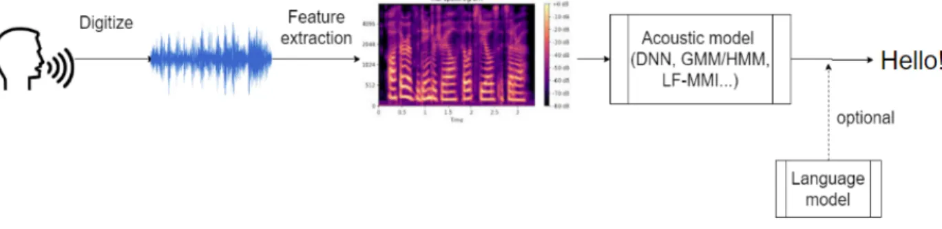
The goal of large vocabulary continuous speech recognition (LVCSR) systems is to map an input acoustic signal to the corresponding orthographic transcription, typically text. A typical LVCSR system often consists of several components as detailed in Figure 1.
Figure 1: A typical ASR system consists of digitization of acoustic signal, feature extraction, acoustic modelling, and optional language modelling.
The acoustic modelling step in Figure 1 aims to perform the mapping of acoustic input
O, which is a sequence of input frames o1, o2, o3, ..., ot, to a sequence of output symbols S (s1, s2, s3, ..., st). Before the emergence of deep learning, this task was often performed using Gaussian Mixture Model (GMM) and then Hidden Markov Model (HMM) to convert input audio features such as Mel-frequency cepstrum coefficients (MFCCs) to characters, which are then corrected using a language model.
Improvements and breakthroughs in deep learning for automatic speech recognition (ASR) have resulted in significant improvements in ASR performance in high-resource languages such as English and Mandarin [31, 27, 10, 6, 14]. Such methods, however, require very large volumes of labelled training data to achieve these notable results. Deep learning ASR sys-tems for languages with limited labelled training data typically must incorporate additional training resources such as cross-lingual acoustic models or in-domain synthetic acoustic data to begin to approach the word error rates found using traditional GMM/HMM frameworks.
The majority of deep learning ASR systems use recurrent neural networks (RNNs) to model temporal dependencies. In a RNN, the state and output of each timestep depends on the state of all previous timesteps in the sequence. Therefore, RNNs can use information from previous inputs as well as the current input to make predictions. For ASR, RNNs can be employed either to make one prediction per timestep, as seen in DeepSpeech 1 and 2 [28, 5], or to obtain an encoding of the audio sequence and then obtain the output text via a decoding network, as seen in Listen-Attend-Spell [10].
Despite good performance in sequence modelling tasks, RNNs often take a long time to train since the output of one timestep is dependent on the output of previous timesteps. As such, the computation of an RNN cell cannot be easily parallelized on modern GPUs. Meanwhile, convolution neural networks (CNNs) can easily take advantage of parallelized computation while still be able to model temporal dependencies by using different kernel sizes. CNNs have demonstrated superior performance on vision tasks such as image classification, im-age segmentation, and object recognition. Early CNN architectures require inputs to be of fixed size. However, as seen in object detection and image segmentation applications, fully convolutional variations can operate on multiple locations simultaneously and allow for variable-size inputs.
3.2
Mel-frequency cepstrum coefficients (MFCCs)
Speech signals can be represented digitally as an array of numbers with the same number of elements per second as the sampling rate. However, this representation does not contain information useful for speech recognition. To counter this problem, the raw audio signal can be converted to the frequency domain using fast Fourier transform (FFT) on small audio window. While the FFT contains energy information at each frequency band in the audio window, it does not put emphasis on the band that is important for human hearing, which is below roughly 1000 Hz. To overcome this problem, Stevens et al. [53] suggested a scale, as shown in (1) , to improve the emphasis on the frequency important to human hearing.
mel(f) = 1127ln(1 + f
700) (1)
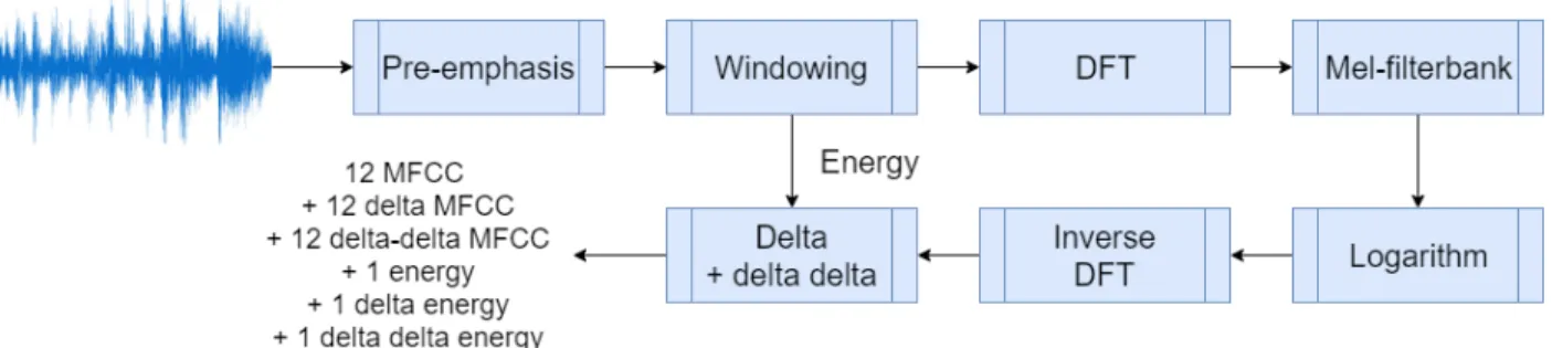
The mel-frequency cepstrum coefficient (MFCC) is a speech signal feature commonly used in ASR research as well as music classification research. Figure 2 shows the process of extracting MFCCs for a speech signal.
Figure 2: The process of extracting MFCCs from a raw audio signal focuses on the frequencies that are important to human hearing.
Since the characteristic of speech changes throughout an utterance, spectral features obtained over the entire utterance would not convey useful information. Instead, features are typically extracted over a small window, typically 25 ms, strided by 10 ms. Each window is then passed
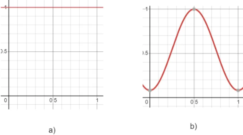
through the pipeline shown in Figure 2. The pre-emphasis step in Figure 2 aims to boost the energy of the signal at high frequency since the high frequency of human speech typically has lower energy than low frequency, but is also important to speech recognition task. After the pre-emphasis step, the windowing step involves multiplying the signal with a pre-defined window. While a rectangular window (Figure 3a) is the simplest window to use, it causes the signal to be abruptly cuts off at the edge. The cutoff causes problems when the discrete Fourier transform of the signal is obtained. Instead, a Hamming window (Figure 3b) is used. A Hamming window approaches 0 at its edges, which shrinks the value of the input signal toward 0 at the boundaries [36].
Figure 3: A rectangular window (a) is simpliest to implement but results in audio being abruptly cuts off at the edges. A Hamming window (b) avoids this problem by fading toward 0 at the edges.
The discrete Fourier transform (DFT) of each window is then computed. To approximate the mel scale described in (1), mel-filterbanks are then used to filter the output from the DFT. Typical mel-filterbanks consists of 10 linearly-spaced filters from 0 to 1000 Hz. Above 1000 Hz, the filters are spaced logarithmically. The spacing of the filters put more emphasis on the lower frequency, similar to how the mel scale operates. The logarithmic of the output is then taken to reduce variations in the input. While the log of the mel spectrum can be used as input features to an ASR system, it does not separate the information from the glottal pulse, which affects the speaker’s fundamental frequency, from the information about
the vocal tract, which shapes the phones. An inverse DFT operation is then performed to obtain the cepstrum of the signal. A cepstrum aims at separating the fundamental frequency, which is more important for speaker identification and ASR for tonal languages, from the shape of the vocal tract, which is important to speech recognition tasks. The lower cepstral values contain information related to the vocal tract, while the higher cepstral values contain information related to the glottal pulse. Prior research [36] have shown that the first 12 cepstral values are typically used in ASR application. In addition to the cepstral values, the average energy level over each window is also added as a feature. Finally, the first and second derivatives of the cepstrum as well as the energy level from each window is taken to obtain 39 MFCCs.
3.3
Connectionist Temporal Classification (CTC)
One of the challenges of LVCSR is the alignment of the audio and ground truth text. Because the input is an audio stream while the output is typically a string of characters or words, manual ground truth alignment can be very time consuming and labor intensive. Since the length of speech can be different between speakers for the same ground truth, each character of the transcription must be aligned to the exact location in the audio for training. For either recurrent or convolutional architectures, the number of input audio windows is often much greater than the number of characters in the target transcripts. The CTC operation [23], allows systems to be trained without the need for alignment.
The CTC loss function avoids the alignment problem by summing over the probability of all possible alignments between the encoded text and the ground truth. To obtain an alignment, an encoded text consisting of repeating characters in consecutive timesteps can be collapsed into a single character. A special CTC blank token (” ”) is used to separate consecutive characters that should not be collapsed.
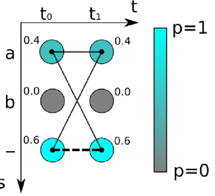
A CTC-trained neural network learns to produce the encoded text from a given input se-quence. At each timestep, the network produces the probability for each character in the alphabet, including the CTC blank. The sum of the probability of all possible alignments corresponding to the ground truth yields a score for the encoded text. The CTC loss is sim-ply the negative log likelihood of the score for the encoded text. Figure 4 shows an example of how CTC score can be computed using an example of 2 timesteps and 3 unique tokens.
Figure 4: The output of a neural network is color coded and also labelled for each timestep. The solid paths represent the alignments corresponding to the ground truth ‘a’, while the dashed path represents the only possible alignment for the output ‘’ 4.
As seen in Figure 4, there are 3 different paths which can lead to the output ‘a’, namely ‘aa’ with probability 0.4×0.4 = 0.16, ‘a ’ (probability 0.4×0.6 = 0.24), and ‘ a’ (probability 0.6×
0.4 = 0.24). There is only 1 path corresponding to the output ‘’, namely ‘ ’ (probability 0.6×
0.6 = 0.36). The CTC score for the output ‘a’ is the sum of the probabilities corresponding
to all paths that produce output ‘a’, which is 0.16 + 0.24 + 0.24 = 0.64. The CTC score 4
for the output ‘’, computed in similar fashion, is 0.36. The CTC loss can be obtained by
computing the negative log of the probability of the path leading to the correct ground truth.
3.4
Language modelling
As shown in Figure 1, an ASR system can include a language model (LM) along with the acoustic model to obtain better performance. While the use of a LM is not necessary to obtain output from the system, it is often critical to obtaining usable output. The goal of a LM is to determine the most likely sequence of words or characters given the output of the acoustic model. With the advancement of deep learning, neural language models such as RNN-based models [45, 54, 24], CNN-based model [18], or attention-based models [19, 50] have been proposed. However, n-gram language models are still common used for decoding in ASR tasks. In an N-gram language models, the probabilities of sequences of 1 to N tokens, where a token is a word, are computed from a given text corpora, such as the transcripts of the training data or written data obtained from books, webpages, historical documents, etc. Additional processing steps such as smoothing and pruning of the probability can be applied to simplify the language models. For the experiments performed in this research, N-gram language models generating with the KenLM tool [30] were utilized.
3.5
Generative Adversarial Networks (GANs)
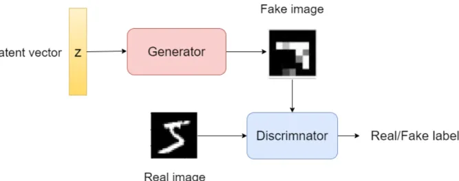
While deep learning becomes prevalent due to discriminative models used in image classi-fication, Goodfellow et al. [21] proposed a generative model that can learn the underlying distribution of the data based on adversarial training. Figure 5 shows the architecture of a basic generative adversarial network (GAN).
A GAN pits a discriminatorDagainst a generatorG. The goal of the generator is to generate
an output that closely resembles a sample from a distribution, while the discriminator seeks to distinguish an input as either the output of the generator or a real sample from the
Figure 5: A generative adversarial network aims to create a realistic image from a latent vector space by training a generator to generate the fake image and a discriminator to detect such fake images.
distribution. These objectives can be represented by (2).
min
G maxD V(D, G) = Ex∼Pdata(x)[logD(x)] +Ez∼Pz(z)log(1−D(G(z)))] (2) In (2), the generator aims to minimize the probability that the discriminator would classify the generated output as fake. The discriminator, on the other hand, aims to maximize the probability of making the correct prediction. As the discriminator gets better at detecting the fake images generated by the generator, the generator also learns to generate more realistic images that can fool the discriminator. As a result, the generator can eventually generate images that closely resemble those used to train the network.
By adding different constraints to the architecture of the network, GANs can be used to generate samples that maintain certain characteristics while changing others. Using convo-lution and transposed convoconvo-lution instead of vanilla feed forward layers, Radford et al. [49] proposed DCGAN, which can represent local dependencies and texture better. Zhu et al.
[66] managed to generate images of a different style while still maintaining the structure of the images by using cycle-consistency loss to ensure images can be converted between two styles. Choi et al. [15] proposed a single network that can perform mutli-domain image translation by adding a domain classifier which can identify which domain the output image belongs to. With the domain classifier, the generator has to learn the characteristics of the target domain.
3.6
Recurrent Neural Network (RNN) and Long-Short Term
Mem-ory cells (LSTM)
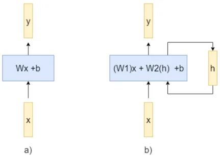
For sequence understanding, it is important to have information from not only the current timestep, but also from tiemsteps before, and optionally after. A typical feed-forward neural network does not have the capability to process information at different timesteps. However, a RNN is designed to learn temporal dependencies. Figure 6 shows the difference between a feed forward layer and a recurrent layer.
Figure 6: A feed-forward layer (a) produces the output vector (y) based on an input vector x. A recurrent layer (b) produces the output vector y based on an input vector x and a hidden state h.
weight matrix, andb is a bias vector. The output of a recurrent layer, however, is computed
using (4), whereW1, W2, W3,W4 are weight matrices,h is a hidden vector, and b and c are
a bias vectors.
y=W x+b (3)
y=W1x+W2h+b (4)
h=W3x+W4h+c (5)
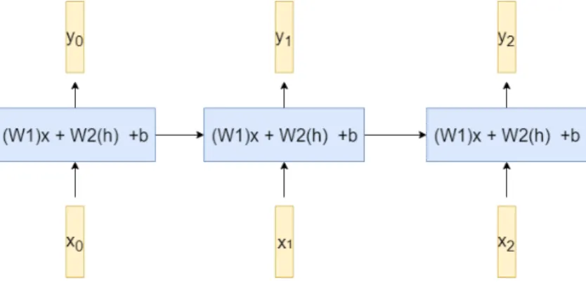
At each timestep, a recurrent layer computes the prediction as well as the next hidden state based on the previous timestep hidden state and the input at the current timestep. Figure 7 demonstrates the use of the hidden state to obtain information across many timesteps. While Figure 7 only shows the information being passed in one direction, a bidirectional RNN can also propagate information from future timestep to past timestep.
Figure 7: At each timestep, a recurrent layer computes its output based on the current timestep input and the hidden state from the previous timestep.
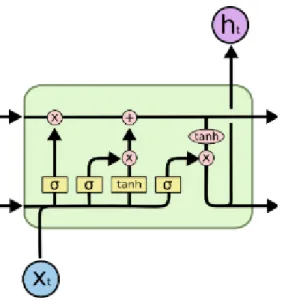
While RNN manages to model sequences fairly effectively, it typically experiences vanishing or exploding gradient problems as the number of timesteps in a sequence grows. The van-ishing gradient problem is caused by small gradients being multiplied together, eventually approaching 0. The exploding gradient, on the other hand, is caused by large gradients being multiplied together, eventually approaching infinity. To tackle these problems, Long-Short Term Memory cells (Figure 8) was introduced.
Figure 8: An LSTM cell contains gates which allow for the control of how much information from previous timesteps is passed through6.
An LSTM consists of a forget gate, represented by the left-most sigmoid activation function, an input gate, represented by the middle sigmoid and tanh function, and an output gate, represented by the last sigmoid. The forget gate controls how much of information from past timesteps to affect the output of the current timestep. The input gate computes the new cell state C from past hidden state and the current input. This cell state is then added to
the previous cell state, whose information has been controlled by the forget gate. Finally, the new cell state and the current timestep input is used to compute the current timestep output and the new hidden state.
3.7
DeepSpeech
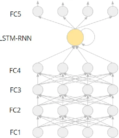
The baseline model for deep learning ASR is DeepSpeech [28], implemented by Mozilla 7. The model (Figure 9) consists of 6 layers: layers 1, 2, 3, and 5 are fully-connected layers of 2048 units, layer 4 is a recurrent layer with 2048 LSTM cells, and layer 6 is a fully-connected layer that predicts a character for a timestep. The input to the model consists of 39 MFCCs taken with window size of 25 ms with 10 ms stride. The model is trained using the CTC loss function. Using this model, different data augmentation techniques were evaluated.
Figure 9: The DeepSpeech architecture consists of fully-connected layers followed by a recur-rent layer that captures temporal dependencies, and a fully-connected layer to predict output characters.
3.8
Audio Spoofing
With the popularity of social media, the spreading of false information has recently become an important research area for public safety and cybersecurity. False information can be in the form of fake written news or fake media. The advancement of technology, in general, and deep learning, in particular, has lead to the creation of tools that allow the generation of images, videos, and audio segments that are not real but cannot be easily identified by human. While some of these tools can be helpful, they also lead to the generation of fake media which could have significant consequences in politics, economy, and public safety.
An audio spoofing attack happens when an attacker uses a fake audio signal to mimic the identity of another person. There are two main categories of audio spoofing attacks: Logical Access (LA) and Physical Access (PA). In the LA case, the spoofed audio is generated using either a text-to-speech or a voice conversion software. With a text-to-speech synthesis software, a text input can be converted to a speech output with a voice similar to that of a target speaker. A voice conversion software allows a speech given by a source speaker to be converted to a different utterance which has the same linguistic content (i.e. textual information) but with a different speaker identity. The PA scenario focuses on security systems that use voice detection. In this scenario, a pre-recorded spech from the target speaker is replayed in order to trick the security system to believe the target speaker is actually speaking. For this research, we focus on the LA scenario since this type of attack allows the adversary to easily create fake media by falsely representing the identity of the speaker or falsely creating the content with a given speaker identity.
LA attacks often involve the usage of text-to-speech (TTS) synthesis systems or voice conver-sion (VC) systems. Most voice converconver-sion systems use a neural-network-based and spectral-filtering-based approaches [44]. Additionally, GANs have also allowed the creation of non-parallel voice conversion systems, which do not require the source and target speakers to say
the same content.
3.9
Constant Q Cepstral Coefficients (CQCC)
The constant Q transform (CQT), first introduced for music processing [8], is a signal pro-cessing technique aimed at producing a spectrum with a constant Q factor. The Q-factor (6) of a filter is defined as the ratio between the the center frequency (fc) and the bandwidth
of the filter w.
Q= fc
w (6)
Human hearing have been shown to approximate a constant Q factor between 500 Hz and 20kHz [46]. The CQT aims at obtaining a spectrum with a constant Q factor by using geometrically spaced frequency bins instead of linearly spaced frequency bins as seen in Fourier-based methods. The advantage of the CQT over Fourier-based transformation is it provides higher frequency resolution at lower frequencies and higher temporal resolution at higher frequencies.
The CQCC can be obtained by first performing the CQT on the input signal. A power spec-trum is then computed from the output of the CQT, and its logarithm is taken. Afterward, a uniform re-sampling of the output is then performed before a discrete cosine transform is taken to obtain the CQCC. Details of how to obtain the CQCC can be found at [57].
4
Previous works
4.1
Resource Constrained ASR
When given sufficient in-domain monolingual training data, deep neural network methods for ASR often perform significantly better than traditional methods based on HMMs and GMMs [31, 22, 27, 4, 10, 65, 14, 2]. Common approaches for deep learning ASR rely on RNNs: sequence-to-sequence models like that in Chen et al. [10] use RNNs to generate a latent representation of the utterance before decoding with RNNs, while DeepSpeech 1 and DeepSpeech 2 [27, 4] use RNNs to capture temporal dependencies before making predictions for each timestep. Methods that produce characters, such as versions of DeepSpeech, cur-rently use Connectionist Temporal Classification (CTC) [23] to reduce streams of characters to plausible words by combining consecutive similar characters and pauses during speech.
Convolutional architectures have achieved remarkable results in computer vision tasks such as image classification [55, 64, 29, 55, 64] and image segmentation [40]. The first successful breakthrough of convolutional neural network came in 2012 when Krizhevsky et al. [38] achieves one of the best results in the ImageNet competition using AlexNet. Szegedy et al. [55] introduced the concept of an Inception block which consists of convolution with multiple filter sizes in a layer to capture different levels of regional dependencies. This concept can be applied to sequential data like speech by using filters with different widths to simultaneously capture different temporal dependencies. The Inception network also introduces 1× bottleneck filters to reduce the number of parameters in a model by reducing the number of filter maps being passed into the main filters in each Inception block. He et al. [29] came up with the idea of skip-connection to improve the flow gradient and improve convergence rate by allowing the model to learn the difference between the output and input rather than learning the transformation from input to output. Xie et al. [64] use Inception-like blocks but with similar filter sizes while adding skip connections similar to ResNet to
allow for better gradient flow.
Previous experiments have shown that transfer learning from a model trained on resource-rich languages can improve the performance of ASR for low-resource languages [20, 32]. Using synthetic data has also been found to yield improvements in true low-resource, arti-ficially low-resource, and resource-rich conditions [61, 7, 63]. Augmentation methods such as adding background noise, changing fundamental frequency, modifying speaking rate, and other distortions of the signal lead to WER reductions for ASR systems trained on less than two hours of audio [33]. Carmantini et al. [9] introduced sample overgeneration dur-ing initialization for low-resource ASR for improved semi-supervised traindur-ing on lattice-free maximum mutual information (LF-MMI) [43]. Malhotra el at. [42] selected samples with lower confidence in an active learning scenario for low-resource ASR.
Rosenberg et al. [51] investigated the use of a CTC-based RNN and an RNN Encoder-Decoder network in character-based end-to-end ASR for low-resource languages. While recurrent-based models have demonstrated usefulness in ASR and other sequence modeling tasks, these models cannot easily take advantage of parallelization on modern hardware since the output of an RNN cell at each timestep depends on the results from the previous timestep. To mitigate this problem, Collobert et al. [16] relies on convolution to capture temporal dependencies.
The fully convolutional, character-based architecture proposed by Collobert et al. [16] still requires training models with large numbers of parameters. Additionally, these models have a high number of layers causing the models to converge more slowly. Our proposed model aims to reduce the complexity of the model without reducing performance by using bottleneck filters and skip connections. Additionally, instead of relying on different layers to capture different levels of temporal dependencies, we combine filters with different widths into one
layer to reduce the number of layers in the model while still maintaining a wide context window.
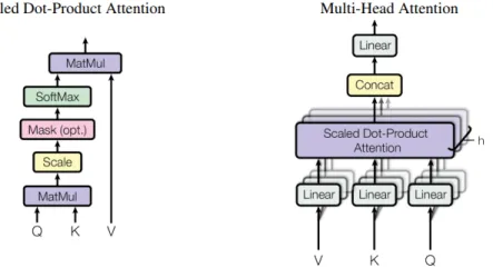
Another approach to mitigate the training time problem with RNN is the use of self-attention models. Vaswani et al. [62] proposes a self-attention model, called Transformer model, as a way to perform sequence-to-sequence tasks without relying on recurrent connections. The Transformer model relies on the concept of Multi-Headed Attention (MHA) (Figure 10) to emphasize important parts of a sequence. Each MHA consists of multiple scaled dot-product attention modules, each compute different attention matrices to allow the MHA to focus on multiple parts of the sequence at once. Since the sequence is represented as a matrix, a MHA module can compute scores for all timesteps at once.
Figure 10: The main building block of Transformer models are Multi-Headed Attention blocks (right), which computes multiple scaled dot-product attentions (left) for each sequence.
Another proposed method for deep learning without a large volume of labelled data is self-supervised learning. In self-self-supervised learning, unlabelled data can be used to train a neural network on pre-tasks. Such pre-tasks do not require knowing the groundtruth of the data. Some examples of pre-tasks are: determining a missing element in a sequence or picture based on surrounding elements, determining the correct order of a scrambled sequence. When trained on such pre-tasks, the neural network can learn rich feature representations of the
input, which can then be used to train the network on the targeted task such as image classification or speech recognition.
Noroozi et al. [47] proposed a method of self-supervised learning for images by training a network to solve a jigsaw puzzle of a small image patch. van den Oord et al. [48] pro-poses a method of self-supervised learning by asking a neural network to predict the next image patch, given several other incorrect image patches, based on previous image patches. Schneider et al. [52] takes this idea and applied it to audio representation, in a method called Wav2Vec, by training two neural networks: an encoding network and a context network (Fig-ure 11. The encoding network downsamples a raw audio while also learning representations from the raw audio, called embeddings. The context network produces a vector which is used to predict the correct embedding of several future timesteps.
Figure 11: In Wav2Vec, the context network (gar) is used to obtain a context vectorct which
is then used to predict future encoding zt. The encoding is obtained from raw audio using an
encoder genc.
While transfer learning and data augmentation separately have both shown improvements, we explore the effectiveness of combining both concepts on low resource ASR, as well as a final finetuning step using only unaugmented data to prevent digital artifacts in augmented data from degrading performance.
4.2
Audio spoofing detection
To counter the spoofing problem, different speech features, such as constant-Q cepstrum coefficients (CQCC) [58], or MFCCs, have been combined with GMM and DNN to produce a detection system. While these systems have performed very well against PA scenarios, there have not been any performance benchmark on LA scenarios. Additionally, the result of the Voice Conversion Challenge 2018 [41] shows many promising parallel and non-parallel voice conversion techniques, which allow fake audio to be created much easier.
In detecting fake images and videos, two main families of neural networks are often used: RNN-based architecture with CNN feature extractors, and pure CNN. One problem with fake audio and images is the frequency or resolution at which digital artifacts remain. To combat this problem in image forgery, Afchar et al. [1] opts to examine the mesoscopic level of images to identify forgery in a network called MesoNet. MesoNet consists of layers with different kernel sizes, which are aimed to examine different resolution levels. This idea can be extended to audio spoofing detection by combining kernels of multiple sizes to detect artifacts at different frequencies.
Another method that has been used to detect fake videos is Convolutional-Recurrent Neural Network (C-RNN) [26]. In this method, a convolutional neural network is used as feature extractor for each frame in the video. The features are then passed into a Long-short Term Memory (LSTM) cell, which will produce a vector which can be used to determine whether the entire video is fake or not. Similarly, for audio, audio features, obtained via signal processing techniques or via a CNN, can be passed into an LSTM and then through a classification layer to determine whether the audio is spoofed.
on cropped or padded audio, convolution-recurrent networks, 1-D CNN, Gaussian Mixture Model, and Support Vector Machines to perform spoofing detection on the ASVSpoof 2019 dataset. For the same dataset, Alzantot et al. [3] uses a 2-D CNN with skip-connection, trained on fixed size crops of audio to perform countermeasure.
5
Datasets
5.1
Resource Constrained ASR
5.1.1 Seneca dataset
The primary target language for this research is Seneca, a morphologically complex and endangered language spoken by Native Americans in the Western New York area. Currently, there are roughly only 50 individuals who speak Seneca as their first language, and a few hundred who speak Seneca as their second language. The raw audio recordings used in our experiments consist of roughly 720 minutes of conversational, spontaneous speech from eleven adult speakers, eight male and three female. All speakers use Seneca as their first language, with English as a second language. All speakers are middle-aged or elderly. The audio was recorded using various equipment, in different environemnts, and was made over many years. As such, the recordings have a diverse range of audio quality. The recordings were segmented at the utterance level and transcribed using Seneca’s current orthographic conventions by second-language Seneca speakers.
The transcribed audio data was partitioned into a 10-hour training set and a 2-hour test set as follows. Using the utterance boundaries provided in the reference transcripts, we randomly selected individual utterances from the full corpus of twelve hours until we had compiled ten hours of audio for training. The remaining two hours comprise the test set. We deliberately selected utterances in a random fashion in order to maximize diversity of gender,
age, dialect, voice quality, and content (e.g., narrative vs. conversation) of both the training and test sets and to avoid overfitting to any particular speaker or speaker characteristic. We note that selecting the test data in this way has the effect that certain speakers appear in both the testing and training data, a compromise we are obliged to make given the very small number of available speakers of the language.
Approximately six hours of the audio data consists of casual conversations between one of the authors and a Seneca elder dealing with current events, the weather, and anecdotes from the elder’s childhood. The remaining audio data was collected from a variety of other speakers and consists of community narratives and information about the natural world. In addition to transcriptions of this audio (roughly 35,000 words), the text data used to train the language model includes an additional 6000 words of previously transcribed texts for which there are no corresponding audio recordings.
5.1.2 Iban dataset
In order to determine how well the architectures and techniques investigated work for low-resource languages in general, the Iban language was also used to evaluate the performance of the system. Iban is a Malayic language spoken in Malaysia, Indonesia, and Brunei. There are about 800,000 estimated native speakers.
The Iban dataset [35] consists of 8 hours of audio obtained from local radio and television stations in Malaysia. The transcription was performed by Iban native speakers. The dataset was split into 71 minutes of testing data, consisting of 6 speakers (2 males, 4 females), and 408 minutes of training data, consisting of 17 speakers (7 males, 10 females).
5.2
Audio Spoofing
5.2.1 ASVspoof2019 dataset
To evaluate the fake audio detection algorithm, we use the ASVspoof 2019 dataset [59]. The dataset consists of two spoofing scenarios: Logical access (LA) and Physical access (PA). In the LA scenario, the fake audio is created using a speech synthesis or speech conversion software. In the PA scenario, the fake audio is created by replaying a pre-recorded audio using an output device, such as a speaker. For this research, the focus will be on the logical access data since it is easier, and more dangerous, to create speeches from any given text using logical access methods. Table 1 shows the composition of speakers’ trait in the dataset.
Table 1: ASVspoof 2019 LA dataset speaker and attack type composition
Partition Male speakers Female speakers Attack algorithms
Training 8 12 Known
Development (Validation) 8 12 Known
Evaluation (Test) 21 27 Known, Unknown
No speaker appears in more than one partition (training, development, or evaluation). All non-spoofed recordings were performed in the same condition. The training and development sets contain spoofed audio generated using the same algorithms. The evaluation set contains audio generated the algorithms used in the training and development sets as well as different algorithms. In total, there were 17 different spoofing systems used, with 6 systems designated as known attacks, and 11 designated as unknown attacks. The six known attack systems consist of 2 VC systems and 4 TTS systems, while the 11 unknown attacks consist of 2 VC systems, 6 TTS systems, and 3 hybrid TTS-VC systems. The training and development sets use only the 6 known attacks, while the evaluation set use 2 known attacks and all 11 unknown attacks. Thus, a good algorithm should be able to detect spoofing via unseen algorithms.
Table 2: ASVspoof 2019 LA dataset ground truth composition
Partition Spoofed samples Bonafide samples
Training 22800 2580
Development (Validation) 22296 2548
Evaluation (Test) 63882 7355
Table 2 shows the ground truth distribution of the dataset. Notably, in all partitions, the number of spoofed samples significantly outnumbers the number of bonafide samples. The ratio of spoofed samples to bonafide samples is approximately 10 : 1. This ratio can potentially lead to challenges in training the model since the model can achieve fairly high accuracy just by predicting any samples to be spoofed.
6
Methodology
6.1
Resource Constrained ASR
6.1.1 Data augmentation
Data augmentation involves generating new, synthetic data from existing data. For speech, data augmentation aims at creating new utterances with the same linguistic content (i.e. transcription) while modifying acoustic characteristics. Jimerson et al. [33] explored data augmentation via distortion of the speech signal, in which they added to the training corpus copies of the existing audio data that were modified to adjust the fundamental frequency (F0) and speaking rate or to include background noise. Here we focus on modifying pitch and speaking rate using the Pitch Synchronous Overlap and Add (PSOLA) algorithm [11]. For pitch augmentation, the F0 of the speech signal was varied in fractions of octaves ranging from 0.10 to 0.30 with a step size of 0.05. Speaking rate was adjusted by re-sampling the audio at multiples of the sampling frequency of the utterance ranging from 0.75 to 1.25 with a step size of 0.05. Each utterance in the training corpus was distorted 10 times
with parameters randomly chosen and added to the existing training corpus, resulting in an additional 6000 minutes of audio data.
Another way of generating synthetic training data is via non-parallel voice conversion. Non-parallel voice conversion techniques do not require the source and target speakers to say the same speech in the training process. As such, these techniques are suitable for gener-ating new data for low-resource languages where getting speakers to say the same speech is difficult. The StarGAN-VC model [37] modifies the image-based StarGAN [15] to acoustic features to perform many-to-many voice conversions. StarGAN implements a cycleGAN [66] architecture with an additional domain classifier, where the speaker identity was used as the domain. Figure 12 shows the overall architecture of StarGAN.
Figure 12: StarGAN uses a domain classifier as well as domain vectors to allow many-to-many style conversion.
As seen in Figure 12, the generatorG takes an input image as well as a vector representing
the target domain (zebra in the given example). Its goal is to generate an image that maintains the structure of the original image while has the style of the target domain. To ensure the same structure, a reconstructed image is created using the generated image and the domain vector from the source domain. The difference between the input image and the
reconstructed image is the reconstruction loss. To ensure the style of the generated image matches the target domain style, a domain classifier is used to determine which domain the generated image belongs to. Lastly, similar to the GAN model proposed by Goodfellow et al. [21], a real/fake discriminator is used to make sure the generated image looks as realistic as possible. The loss function used to train the discriminator, which consists of a real/fake classifier and a domain classifier, is shown in (7), and the loss function for the generator is shown in (8).
LD =−Ladv+λclsLclsreal (7)
LG =Ladv +λclsLclsf ake+λrecLrec (8)
In (7) and (8), Ladv represents the loss obtained from the real and fake detection. Lcls represents the loss of the domain classifier, which is ann-class classifier, wherenis the number
of domains. The recovery loss, which captures the differences between the reconstructed image and the original input image, is represented by Lrec. λcls and λrec represent the weights given for each of the loss to adjust the emphasis on either the domain similarity or the reconstruction similarity.
By replacing images with spectrograms and representing speaker identity with domain vec-tors, Kameoka et al. [37] proposed the architecture of StarGAN can be employed to perform many-to-many voice conversion. The output of StarGAN-VC is then converted back to raw audio using the Griffin-Lim algorithm [25].
For each of the voice conversion methods, we selected the three speakers with the largest volume of labelled data: Speaker A (94 minutes), Speaker B (250 minutes), and Speaker C (156 minutes). Since StarGAN-VC enables many-to-many voice conversion, only one StarGAN-VC model was trained to perform voice conversion among the three speakers. The StarGAN-VC model was trained for a total of 500,000 iterations, with sample outputs taken at every 50,000 iterations to subjectively determine whether the model produced intelligible utterances. A total of six VAWGAN models were trained to perform voice conversion among the three speakers since VAWGAN only allows for one-to-one voice conversion. Each VAW-GAN model was trained for 100 epochs, with samples taken every 10 epochs to determine whether synthesized utterances were intelligible. The trained StarGAN-VC and VAWGAN models were then used to convert utterances from each of the three speakers to the other two. From the original 500 minutes of audio produced by Speakers A, B, and C, we obtained 1000 minutes of synthetic data for each voice conversion model.
6.1.2 Acoustic modelling
Mini-Gated Convolutional Neural Network (m-GCNN) Based on the models sug-gested by Collobert et al. [16] and Liptchinsky et al. [39], fully convolutional approach for ASR was explored. Since speech and acoustic signals can be represented as a 1-D array of numbers, 1-D convolution operations can be used to learn temporal dependencies similar to how 2-D convolution operations have been used to learn spatial dependencies for vision tasks. At each timestep, the combination of all feature maps in a finite temporal window can be used to obtain a feature map in the next layer. After several layers, the network makes a character prediction at each timestep. These character predictions can then be decoded using the CTC function. Since predictions are made for each timestep, the input to the network can be sequences of variable lengths.
compact version of the Gated Convolutional Neural Network (GCNN) proposed in [39], called mini-GCNN or mGCNN. Figure 13 shows the overall architecture of mGCNN.
Figure 13: The mGCNN consists of 8 Gated Linear Unit (GLU) blocks with different kernel widths and a final linear layer which predicts one character per timestep
Compared to the original GCNN, mGCNN removes layers with kernel sizes from 8 to 20. This change was made to simplify the model in an attempt to reduce the number of parameters, making it more suitable for the small volume of training data. After the feature extraction step, a mid-size Gated Linear Unit (GLU) block is used to capture contextual information
before a series of GLU blocks with increasing kernel size extracts features with increasingly wider temporal dependencies. Finally, a GLU block with kernel size 1 and a linear layer (represented as a convolution block with kernel size of 1) perform the prediction. Figure 14 shows the components of a GLU.
Figure 14: A GLU consists of two paths: one performs the feature extraction (Conv B) while the other (Conv A) determines how much information from each feature map is passed to the next layer.
A GLU consists of two convolution operations of the same kernel size. One of the convolution (the bottom path in Figure 14) performs feature extraction similar to a normal convolution operation. The other convolution (the top path in Figure 14), however, learns the importance of each feature map produced by the other path. As such, the output of this path is passed through a sigmoid layer, which is then multiplied with the output of the feature extraction path. With the ability to learn the importance of individual feature maps, a GLU allows for better convergence and gradient flow in the network. Optionally, a skip connection can also be used between the input and the output of the GLU to further improve the gradient flow.
Wide Inception REsidual Network (WIRENet) While mGCNN uses GLU blocks of different kernel sizes in series to capture different level of temporal dependencies, convolution operations can also be performed in parallel path, as demonstrated in Inception models [56]. Based on this intuition, we propose a novel network, called Wide Inception Residual Network or WIRENet, comprised of multiple blocks of convolutions with different filter sizes. Figure 15 shows the architecture of a Wide Block, the key building block of this network.
Figure 15: A Wide Block contains multiple paths, each with different convolution kernel size, to learn different ranges of temporal dependencies.
The main building block of our architecture is the WideBlock (Figure 15), named for the high number of paths in each block. The architecture of the block, taking inspiration from ResNeXt blocks used in image classification [64], consists of several parallel streams, each consisting of bottleneck 1×1 convolution layers before and after a normal convolution layer. The bottleneck layers reduce the complexity of the model by reducing the number of param-eters required by the middle convolution operation. Instead of keeping the same filter size for all paths, we draw inspiration from Inception networks and employ filters with different sizes in each layer. The filter widths are odd numbers between 3 and 19. This choice is suitable for speech-related tasks since temporal dependencies in audio typically have more variance than spatial dependencies in visual tasks. The different filter sizes allow the model to pick up both short-term and long-term temporal dependencies. The output from each path is then summed before being added to the input of each block, forming a skip connection.
Figure 16: WIRENet consists of 1-D convolution layers and Wide Blocks. The dimensions of the filters are: input channels, kernel width, output channels.
small-size convolution layer after the feature extraction step. These embedding layers convert input audio features into a vector of desired depth and temporal content. The WIRENet architecture continues with five WideBlocks, then two 1×1 convolution layers which act as fully-connected layers. The final layer outputs a vector with size corresponding to the number of tokens to be predicted. Optionally, a context path, consisting of a convolution
layer with very wide kernel width, can be used in parallel with the Wide Blocks to obtain context information from a wide temporal window before the prediction is made. Batch normalization and ReLU are used after each convolution operation. To prevent overfitting due to limited data, dropout layers of 0.25 are added after each Wide Block. To train the network, the CTC loss function is used.
6.1.3 Multi-staged learning
A proposed learning strategy to mitigate the lack of training data is to train the models in multiple stages. Figure 17 shows the proposed multi-stage learning scheme.
Figure 17: Multiple learning stages can help extract useful features related to human speech (stage 1), the specific language (stage 2), and cleaning up the artifact from augmentations (stage 3)
In the first stage, an acoustic model is trained on 960-hour of LibriSpeech English corpus, with randomized initial weights. The models are trained for 75 epochs, with the best models saved to initialize weights in later stage. The best models were determined by word-error rate on the LibriSpeech validation set.
In the second stage, the weights of a second acoustic model are initialized using the weights from the best English models obtained in the first stage. The training data from this sec-ond model includes the original unaltered 10-hour Seneca dataset as well as up to a 10× augmentation of each utterance using one of the three data augmentation methods: speed and pitch modification (Augment10), or voice conversion via StarGAN-VC. This model is trained until convergence on the training dataset.
The motivation for the final stage is that the augmented data often contains heavy digital artifacts. Since the amount of augmented data is significantly higher than the amount of original data, the networks trained on augmented and original data might be skewed towards improving performance on augmented data. However, it is hoped that the network can still learn valuable representation with augmented data, which will allow the final network trained on original data to perform better.
In the final stage, the weights of the third acoustic model are initialized using the final weights from the second model. The training data for the third models includes only the original 10 hours of unaltered Seneca dataset with no augmented data. Models in this fine-tuning stage are trained until convergence on the training dataset. For the final stage, the learning rate is reduced by an order of magnitude.
6.2
Audio Spoofing
6.2.1 Convolution-Recurrent Neural Network
The first proposed model for spoofing detection is a convolution-recurrent neural network. Figures 18 show the architecture of the proposed model. The model takes raw audio signal as an input and produces the log probability of two classes: bonafide speech and spoofed speech.
Figure 18: The architecture of the proposed convolution-recurrent network consists of con-volution layers to extract features and downsample the input audio, and a recurrent layer to obtain information from all the timesteps.
Since raw audio is used instead of spectral features as the input to the network, five 1-D convolution layers are used to learn useful representation. Additionally, the convolutions are strided to downsample the input signal from 16kHz to 100 Hz, reducing the memory footprint while also speeding up the training process. The extracted features are then passed
to a bidirectional Long-Short Term Memory (LSTM) layer. After the features from the last timestep is passed through the LSTM, the hidden state of the LSTM is used to perform prediction using two fully-connected layers. Dropout and batch normalization are used after each layer to perform regularization. The network is trained using negative log-likelihood loss function. Due to the unbalanced nature of the dataset, a miss classification of a spoofed speech incurs heavier loss than a miss classification of a bonafide speech.
Figure 19: The architecture of the proposed convolution approach for spoofing countermeasure uses Wide Blocks to extract information from different temporal window.
6.2.2 Convolutional-based detection
Similar to the low-resource ASR problem, convolution neural networks are also examined for spoofing countermeasure. Since Wide Block shows promising results for ASR tasks, it is used as a key building block for the CNN countermeasure (Figure 19). Since a countermeasure
only needs to produce one score for an entire utterance instead of one prediction per timestep, the architecture in Figure 19 uses strided convolution and max pooling operations to reduce the length of the feature map as it passes through the network. For similar reason, the input audio is either clipped or repeated to a fixed length of four seconds before the log-mel spectrogram is obtained. Dropout and batch normalization are used after each layer to avoid overfitting. Similar to the CRNN model, the convolution model is also trained using weighted negative log-likelihood.
7
Evaluation metrics
7.1
Low-resource ASR
7.1.1 Character/Word Error Rate
The performance of augmentation methods, acoustic models, and learning strategy is eval-uated using word-error-rate (WER) and character-error-rate (CER). Both metrics are com-puted by aligning the output of the ASR system with the manually generated reference transcript. WER is the minimum edit distance over a word alignment, aggregated across utterances and normalized by the total number of words in the reference. CER is computed in the same manner, except the error is computed over characters instead of words. The minimum edit distance, normalized by the number of tokens, between two sequences is de-fined in (9), whereI,D, andS represent the number of insertion, deletion, and substitution
from to obtain one sequence from the other.
ED= I+D+S
7.2
Audio spoofing detection
7.2.1 Equal Error Rate (EER)
To evaluate the effectiveness of a spoofing detection algorithm, the equal error rate (EER) is used. EER is typically used to evaluate biometric security system. For a biometric system, EER is used to determine the threshold value at which the false acceptance rate, or false positive rate (FPR), shown in (10), is equals to the false rejection rate, or false negative rate (FNR), shown in (11). When F P R=F N R, the common error rate is the EER of the
system. Typically, lower EER corresponds to better accuracy of the system.
F P R= F P
F P +T N (10)
F N R= F N
F N+T P (11)
7.2.2 Tandem Detection Cost Function (t-DCF)
When a spoofing countermeasure is evaluated alone, EER is a good metric to evaluate different systems. However, spoofing countermeasures are often used in tandem with an automatic speaker verification (ASV) system. Thus, the effectiveness of a countermeasure system also needs to be evaluated with the ASV system in mind. To this end, the t-DCF is proposed as an evaluation metric by the organizer of ASVSpoof 2019 challenge [59]. Equation 12 shows how the t-DCF is computed, where Pmisscm and Pf acm corresponding to the FNR and
FPR of the countermeasure system, respectively. β represents the performance of the ASV
system. For the ASVSpoof 2019 challenge, the organizer provides the ASV score, so β is a
specific attack.
t−DCFnormmin = min s {βP
cm
miss(s) +P cm
f a (s)} (12)
8
Results and Analysis
8.1
Low-resource ASR
8.1.1 DeepSpeech with data augmentation
Figure 20 shows the mel-spectrogram of an unaltered Seneca utterance along with its corre-sponding synthetically generated spectrograms for randomly chosen speed and pitch distor-tions, as well as the StarGAN-VC and VAWGAN augmentation methods.
As seen in Figure 20, the speed augmentation resulted in a longer utterance while still main-taining the shape of the spectrogram. The fundamental frequency of the pitch augmentation is higher compared to the original sample. The two voice conversion methods synthesize the utterance from speaker A as if it were spoken by speaker B. The peak locations in the two voice conversion methods are maintained, but the signature characteristics of the voice are transformed.
Table 3 shows the result of different augmentation methods and transfer learning stages on DeepSpeech. For each acoustic model, we evaluate with: 1) no language model (no lm);
and 2) a tri-gram language model ((3-gram). All WERs greater than 1.0 are replaced with
1.0, indicating no useful output was produced.
Figure 20: Mel-spectrograms of a randomly selected utterance. The original utterance (mean F0=153, duration=2048msec) is on the bottom right, while the various augmentation meth-ods, counter-clockwise from bottom left, are: pitch modification (mean F0=179), speaking rate modification (duration=3132msec), and StarGAN-VC.
Table 3: WER and CER across different acoustic models (Kaldi and DeepSpeech) and aug-mentation strategies (rows) vs. language models (columns).
WER CER
no lm 3-gram no lm 3-gram
Baseline: Kaldi N/A 0.530 N/A 0.307
Baseline: DeepSpeech 1.000 0.970 0.891 0.872 Baseline: DeepSpeech w/TL 0.859 0.727 0.436 0.409 TL + Augment10 1.000 0.975 0.716 0.698 TL + Augment10 + finetune 0.850 0.693 0.427 0.421 TL + StarGAN-VC 0.911 0.790 0.497 0.474 TL + StarGAN-VC + finetune 0.772 0.571 0.364 0.333
a WER greater than 1.0, meaning it yielded no usable output. Applying a language model slightly reduces the error rate for this model. Applying transfer learning from English yields