Journal of Risk Volume 15/Number 3, Spring 2013 (39–68)
Asset allocation with conditional value-at-risk
budgets
Kris Boudt
Faculty of Business, Vrije Universiteit Brussel, Pleinlaan 2, 1050 Brussels, Belgium; email: [email protected]
and
Faculty of Economics and Business, VU University Amsterdam, de Boelelaan 1105, 1081 HV Amsterdam, The Netherlands Peter Carl
William Blair & Company, 222 West Adams Street, Chicago, IL 60606, USA; email: [email protected]
Brian G. Peterson
DV Trading, 216 W Jackson Boulevard, Chicago, IL 60606, USA; email: [email protected]
(Received October 19, 2011; revised May 24, 2012; accepted June 11, 2012)
Risk budgets are frequently used to allocate the risk of a portfolio by decompos-ing the total portfolio risk into the risk contribution of each component position. Many approaches to portfolio allocation useex postmethods for constructing risk budgets and take the variance as a risk measure. In this paper, however, we useex antemethods to evaluate the component contribution to conditional value-at-risk (CVaR) and allocate risk. The proposed minimum CVaR concen-tration portfolio draws a balance between the investor’s return objectives and the diversification of risk across the portfolio. For a portfolio invested in bonds, commodities, equities and real estate, we find that over the period from January 1984 to June 2010, the minimum CVaR concentration portfolio offers an attrac-tive compromise between the good risk-adjusted return properties of the minimum CVaR portfolio and the positive return potential and low portfolio turnover of an equally weighted portfolio.
The authors thank David Ardia, Bernhard Pfaff, Dale Rosenthal and two reviewers for helpful com-ments. Financial support from the National Bank of Belgium is gratefully acknowledged. The code to replicate the analysis is available in the R packages PerformanceAnalytics (Carl and Peterson 2010) and PortfolioAnalytics (Boudtet al2011). More information on the utilization of these packages for the estimation and optimization of portfolio risk budgets can be found at www.econ.kuleuven.be/ kris.boudt/public/riskbudgets.htm.
1 INTRODUCTION
Risk budgets are frequently used to allocate the risk of a portfolio by decomposing the total portfolio risk into the risk contribution of each component position. While volatility-weighted portfolio allocation methods have existed for many years, the
ex anteuse of risk budgets in portfolio allocation is more recent.
The risk parity portfolio of Qian (2005) allocates the portfolio variance equally across the portfolio components. Maillardet al(2010) show that the volatility of this portfolio is located between the volatilities of the minimum variance and the equally weighted portfolio. Zhuet al(2010) study optimal mean–variance portfolio selection under a direct constraint on the contributions to portfolio variance. Compared with the equally weighted portfolio, the most diversified portfolio of Choueifaty and Coignard (2008) and the global minimum variance portfolio, Lee (2011) finds that the risk-contribution approach is
potentially more applicable because of its heuristic nature, economic intuition, and the financial interpretation that ties its concept to economic losses.
However, to our knowledge, the literature on risk contribution portfolios lacks a detailed study on the use of downside risk budgets rather than portfolio variance budgets as an ex ante portfolio allocation tool. Given the nonnormality of many financial return series, the practice of assigning equal weights to positive and negative returns when computing risk contributions is likely to be suboptimal with respect to the allocation of risk through ex ante downside risk budgets. We fill this gap by explaining in detail the implementation of portfolio strategies that use downside risk contributions rather than variance contributions as an objective or constraint.
Our focus is on portfolio conditional risk (CVaR), since unlike value-at-risk (VaR), CVaR has all the properties a value-at-risk measure requires to be coherent and is a convex function of the portfolio weights (Artzneret al1999; Pflug 2000). Moreover, CVaR provides less incentive to load on to tail risk above the VaR level. By integrating the CVaR budget into their optimal portfolio policy, investors can directly optimize downside risk diversification.
For many practical applications, the risk parity constraint that requires all assets to contribute equally to portfolio risk is too restrictive. As an alternative, we propose to minimize the largest CVaR risk contribution in the portfolio. Unconstrained, this portfolio criterion still generates portfolios that are similar to the risk parity port-folio, but it has the advantage that it can be more easily combined with many other investor objectives and constraints (such as return targets or drawdown and cardinality constraints).
The outline of the paper is as follows. First, we review the definition and estimation of CVaR portfolio budgets in Section 2. In Section 3 we describe several portfolio
Asset allocation with conditional value-at-risk budgets 41
allocation strategies that use the portfolio component CVaR risk budget as an objective or constraint in the portfolio optimization problem. We conclude with a thorough performance study of the use of CVaR allocation methodology to find the optimal mix of bonds, commodities, equities and real estate. Portfolios are rebalanced quarterly, taking into account the salient features of financial return data, such as time-varying volatility and correlation, skewness and heavy tails. We find that over the period 1984–2010, the minimum CVaR concentration (MCC) portfolio offers an attractive compromise between the good risk-adjusted return properties of the minimum CVaR portfolio and the positive return potential and low portfolio turnover of an equally weighted portfolio.
2 PORTFOLIO CONDITIONAL VALUE-AT-RISK BUDGETS 2.1 Definition
The first step in the construction of a risk budget is to define how portfolio risk and its risk contributions should be measured. A naive approach is to set the risk contribution equal to the stand-alone risk of each portfolio component. This approach is overly simplistic and neglects important diversification or multiplication effects of the component units being exposed differently to the underlying risk factors. Using game theory, Denault (2001) has shown that the only satisfactory risk allocation principle is to measure the risk contribution as the weight of the position in the portfolio times the partial derivative of the portfolio risk Rw with respect to that
weight:
C.i /Rw Dw.i / @Rw @w.i /
: (2.1)
The standard deviation, VaR and CVaR of a portfolio are all linear in position size. By Euler’s theorem, we have that for such risk measures the total portfolio risk equals the sum of the risk contributions in (2.1).
Chow and Kritzman (2001), Litterman (1996), Maillardet al(2010), Peterson and Boudt (2008) and Scherer (2007) study the use of portfolio standard deviation and VaR budgets. In his bookRisk Budgeting, Pearson (2002, p. 7) notes that
value-at-risk has some well known limitations, and it may be that some other risk measure eventually supplants value-at-risk in the risk budgeting process.
We develop a risk budgeting framework for portfolio CVaR. Portfolio CVaR can be expressed in monetary value or percentage returns. Our goal is to apply the CVaR budget in an investment strategy based on quantitative analysis of the asset returns. We therefore choose to define CVaR in percentage returns.
Denote byrw tthe return at timeton the portfolio with weight vectorw. To simplify
notation, we omit the time indextwhenever no confusion is possible and assume that
the density function ofrw is continuous. At a preset probability level denoted by˛,
which is typically set between 1% and 5%, the portfolio VaR is the negative value of the˛quantile of the portfolio returns. The portfolio CVaR is the negative value of the expected portfolio return when that return is less than its˛quantile:
CVaRw.˛/D EŒrw jrw 6VaRw.˛/; (2.2)
with E the expectation operator. The CVaR contribution is the weight of the position in the portfolio times the partial derivative of the portfolio CVaR with respect to that weight:
C.i /CVaRw.˛/Dw.i /
@CVaRw.˛/ @w.i /
; (2.3)
wherew.i /is the portfolio weight of positioniand there areNassets in the investment
universe .i D 1; : : : ; N /. For ease of interpretation, the CVaR contributions are standardized by the total CVaR. This yields the percentage CVaR contributions:
%C.i /CVaRw.˛/D
C.i /CVaRw.˛/
CVaRw.˛/
: (2.4)
The CVaR contributions are directly linked to the downside risk concentration of the portfolio. Scaillet (2002) shows that the contributions to CVaR correspond to the conditional expectation of the return of the portfolio component when the portfolio loss is larger than its VaR loss:
C.i /CVaRw.˛/D EŒw.i /r.i /jrw 6VaRw.˛/: (2.5)
An interesting summary statistic of the portfolio’s CVaR allocation is what we call the portfolio CVaR concentration, defined as the largest component CVaR of all positions:
Cw.˛/Dmax
i C.i /CVaRw.˛/: (2.6)
As we will show later, minimizing the portfolio CVaR concentration leads to portfolios with a relatively low CVaR and a balanced CVaR allocation.
2.2 Estimation
The actual risk contributions can be estimated in two ways. One approach is to estimate the risk contributions by replacing the expectation in (2.5) with the sample counter-part evaluated using historical or simulated data. In a portfolio optimization setting, the risk contributions need to be evaluated for a large number of possible weights, and therefore fast and explicit estimators are needed. A more elegant approach for
Asset allocation with conditional value-at-risk budgets 43
optimization problems is therefore to derive the analytical formulas of the risk con-tributions. If the returns at timet are conditionally normally distributed with mean
t and covariance matrix˙t, then CVaR at timet is given by
CVaRw.˛/D w0tC p w0˙ tw .z˛/ ˛ ;
withz˛the˛quantile of the standard normal distribution andthe standard normal
density function. The contribution to CVaR is then
C.i /CVaRw.˛/Dw.i / .i /tC .˙tw/.i / p w0˙ tw .z˛/ ˛ : (2.7)
Financial returns are usually nonnormally distributed. In the empirical application, we use the modified CVaR (contribution) estimator proposed by Boudtet al(2008). Based on Cornish–Fisher expansions, the modified CVaR estimate is an explicit func-tion of the components of the underlying asset returns. It has been shown to deliver accurate estimates of CVaR (contributions) for portfolios with nonnormal returns. For the exact definition of this estimator, refer to Appendix A. The Cornish–Fisher-based estimates of CVaR work well for tail probabilities that are not too small, as shown by Boudtet al(2008). Throughout the paper, we set the loss probability˛to 5%. This is a common choice in practical portfolio optimizations, as mentioned, for example, by Keel and Ardia (2011) and Topaloglouet al(2002). For smaller values of˛, the Cornish–Fisher CVaR estimator becomes less reliable and eventually breaks down. A detailed study of the sensitivity of the portfolio performance to the choice of˛is left for further research.
3 CONDITIONAL VALUE-AT-RISK BUDGETS IN PORTFOLIO OPTIMIZATION
Previously, risk budgets based on portfolio standard deviation and VaR have been used as either anex postor anex antetool for tuning the portfolio allocation.
In theex postapproach, the portfolio is first optimized without taking into account the risk allocation. The risk budget of the optimal portfolio is then estimated and risk budget violations are adjusted on a marginal basis. The rationale for this is that the risk contributions in (2.1) can be interpreted as the marginal risk impact of the corresponding position. Because of transaction costs, traders and portfolio managers often update their portfolios incrementally, which makes the marginal interpretation of risk contribution useful in practice (Litterman 1996; Stoyanovet al2009). When the risk contribution of a position is zero, Litterman (1996) calls this the “best hedge” position for that portfolio component. The positions with the largest risk contribu-tions are called “hot spots”. If a risk contribution is negative, a small increase in the
corresponding portfolio weight leads to a decrease in the portfolio risk. Keel and Ardia (2011), however, show that reallocation of the portfolio based on these risk contributions is limited in two ways. First of all, as a sensitivity measure, the risk contributions are precise for infinitesimal changes, but these approximations can be poor for realistic reallocations. Second, they assume changes in a single position while keeping all other positions fixed. In the presence of a full investment constraint, this is unrealistic.
While various volatility-weighted portfolio allocation methods have existed for many years, theex anteuse of risk budgets in portfolio allocation is more recent. Qian’s (2005) “risk parity portfolio” allocates portfolio variance equally across the portfolio components. Maillardet al(2010) call this the “equally-weighted risk contri-bution portfolio” or, simply, the equal-risk contricontri-bution (ERC) portfolio. They derive the theoretical properties of the ERC portfolio and show that its volatility is located between those of the minimum variance and equal-weight portfolios. Zhuet al(2010) study optimal mean–variance portfolio selection under a direct constraint on the con-tributions to portfolio variance.
Our first contribution to the recent literature is to use (percentage) CVaR contri-butions rather than variance contricontri-butions as an objective or constraint in portfolio optimization. By integrating the CVaR budget into their optimal portfolio policy, investors can directly optimize downside risk diversification. The rationale for this is the result in (2.5) that the CVaR contributions correspond to the conditional expecta-tion of the return of the portfolio component when the portfolio loss is larger than its VaR loss. From (2.3) and (2.5), it also follows that the percentage CVaR contribution can be rewritten as the ratio of the expected return on the position at the time the portfolio experiences a beyond-VaR loss to the expected value of the beyond-VaR portfolio losses:
%C.i /CVaRw.˛/D
EŒw.i /r.i /jrw 6VaRw.˛/
EŒrw jrw 6VaRw.˛/
: (3.1)
In almost all practical cases, the denominator in (3.1) is negative, so that a high positive percentage CVaR contribution indicates that the position has a large loss when the portfolio also has a large loss. The higher the percentage CVaR, the more the portfolio downside risk is concentrated on that asset and vice versa.
Our second contribution is the proposal of two strategies for the use of CVaR budgets in portfolio optimization in order to balance the maximum return, minimum downside risk and maximum downside risk diversification objectives of an investor. The first strategy is the MCC portfolio, which uses the downside risk diversification criterion as an objective rather than a constraint. More formally, the MCC portfolio allocation is given by
wMCC Dargmin
w2W
Asset allocation with conditional value-at-risk budgets 45
with the portfolio’s CVaR concentrationCw.˛/as defined in (2.6).W is the set of
feasible portfolio weights. Unless otherwise mentioned,W is only restricted by a full investment constraint.
The second strategy consists of imposing bound constraints on the percentage CVaR contributions. This may be viewed as a direct substitute for a risk diversification approach based on position limits. It has the ERC constraint as a special case:
%C.1/CVaRw.˛/D D%C.N /CVaRw.˛/D1=N: (3.3)
Note that that for a portfolio that has the ERC property, the relative weights are inversely proportional to the marginal impact of the position on the portfolio CVaR:
w.i / w.j /
D @CVaRw.˛/[email protected] / @CVaRw.˛/[email protected] /
: (3.4)
It follows that the ERC allocation strategy yields portfolios that give higher weights to assets with a small marginal risk impact and downweights the investments with a high marginal risk (the so-called hot spots in Litterman (1996)).
In the following subsections, we study the properties of these two approaches in more detail. In the empirical section, we will compare these CVaR budget-based portfolio allocation rules with the more standard minimum CVaR (MC) and equal-weight (EW) portfolios:
wmin CVaR Dargminw2W CVaRw.˛/ and wEW D.1=N; : : : ; 1=N /0: (3.5)
3.1 Properties of the MCC portfolio
For the derivation of the properties of the MCC portfolio, it is useful to rewrite the portfolio CVaR concentration as the portfolio CVaR multiplied by the largest percentage CVaR contribution:
Cw.˛/DCVaRw.˛/maxf%C.1/CVaRw.˛/; : : : ;%C.N /CVaRw.˛/g: (3.6)
The first factor in (3.6) is minimized by the minimum CVaR portfolio. The second factor attains its lowest value when the portfolio has the ERC property, since
maxf%C.1/CVaRw.˛/; : : : ;%C.N /CVaRw.˛/g>1=N:
By minimizing the product of these two factors, the MCC portfolio strikes a balance between the objectives of portfolio risk diversification and total risk minimization. Compared with the unconstrained minimum CVaR portfolio, we obtain that the CVaR of the MCC portfolio is higher, but the risk is less concentrated. In fact, we show in
Appendix A that the percentage CVaR of the fully invested minimum CVaR portfolio coincides with the component’s portfolio weight:
%C.i /CVaRwmin CVaR.˛/Dwmin CVaR.i / : (3.7) It is well-known that the minimum CVaR portfolio generally suffers from the draw-back of portfolio concentration. By (3.7), this carries directly over to the CVaR allo-cation.
In many cases, the CVaR concentration is not a convex function of the portfolio weights, andCw.˛/may also not be differentiable. For this reason, we recommend
the use of a derivative-free global optimizer to find the MCC portfolio. We used the differential evolution algorithm developed by Priceet al(2005). Ardiaet al(2011) provide an example of how to implement the MCC portfolio.
The MCC objective can easily be combined with a return target. This serves the gen-eral purpose of maximizing return subject to some level of risk, while also minimizing the risk concentration at that risk level. We define the mean–CVaR concentration effi-cient frontier as the collection of all portfolios that achieve the lowest degree of CVaR concentration for a return objective. For a given return target rN, the mean–CVaR concentration efficient portfolio solves
min
w2W Cw.˛/ such thatw
0>r:N
(3.8) The minimum CVaR portfolio under the ERC constraint in (3.4) is an alternative to the MCC portfolio for attaining a balance between the objectives of portfolio risk diversification and total risk minimization. In our data examples, the two portfolios were always very similar.
The advantage of the MCC portfolio over the ERC constrained minimum CVaR portfolio is that it is computationally simpler and also will yield a solution if the ERC constraint is not feasible or conflicts with other constraints. Since most real-world portfolios are constructed with an explicit or implicit return objective and other con-straints, the ability to combine with other objectives and constraints is an important consideration for asset managers that is often incompatible with the published litera-ture on utilizing risk metrics in portfolio construction. Note also that the properties of the MCC portfolio generalize to any minimum risk concentration portfolio, as long as the portfolio risk measure is a homogeneous function of order one of the portfolio weights.
3.2 Portfolio allocation under CVaR allocation constraints
The risk allocation can also be controlled by imposing explicit constraints on the per-centage CVaR allocations. This process operates in much the same way that portfolio managers impose weight constraints on portfolios.
Asset allocation with conditional value-at-risk budgets 47 FIGURE 1 Percentage CVaR contribution of asset 1 as a function of its portfolio weight for a two-asset portfolio with asset returns that have a bivariate normal distribution with means1and2, correlationand standard deviations1and2, respectively.
Weight asset 1 0.0 0.2 0.4 0.6 0.8 1.0 0.0 0.2 0.4 0.6 0.8 1.0 % CVaR asset 1 0.0 0.2 0.4 0.6 0.8 1.0 0.0 0.2 0.4 0.6 0.8 1.0 0.0 0.2 0.4 0.6 0.8 1.0 0.0 0.2 0.4 0.6 0.8 1.0 0.0 0.2 0.4 0.6 0.8 1.0 % CVaR asset 1 % CVaR asset 1 % CVaR asset 1 Weight asset 1 Weight asset 1 Weight asset 1 0.0 0.2 0.4 0.6 0.8 1.0 (a) (b) (c) (d)
(a)1D2D0,1D2D1 andD0.5. (b)1D2D0,1D1,2D2 andD0.5. (c)1D1,2D0,
1D2D1 andD0.5. (d)1D2D0,1D2D1 andD0.
Such percentage CVaR contribution constraints reduce the feasible space in a way that depends on the return characteristics. Stoyanovet al(2009) study in detail the effect of the component return characteristics on the total portfolio CVaR. To build further intuition via a stylized example, we plot in Figure 1 the percentage CVaR contributions for a two-asset portfolio with asset returns that have a bivariate nor-mal distribution with means1 and2, standard deviations 1 and2 and a
cor-relation. Of course, the percentage CVaR contribution is 0 and 1, respectively, if the weight is 0 and 1. In between these values, the percentage CVaR displays an S-shape.
The dotted lines in Figure 1 illustrate the effect on the feasible space for portfolio weight 1 of imposing an upper 60% bound on the percentage CVaR contributions of the two assets. This implies that the percentage CVaR contribution of asset 1 has to be between 40% and 60%. In parts (a) and (d), the two assets are identical. In this case,
the feasible space is centered around the equal-weight portfolio. ForD0(part (d)), the percentage CVaR contribution of asset 1 as a function of its weight is more curved than that forD0:5(part (a)).
In the other figures, asset 1 is more attractive than asset 2 since it has either a lower volatility or a higher expected return. We see that this leads to a shift of the feasible space to the right, with allows portfolio weights around 60%. The set of possible weights satisfying the box constraints on the percentage CVaR contributions changes in an intuitively appealing way when differences in return and volatility are allowed. For general portfolios with nonnormal returns, there is no explicit representation of the percentage CVaR constraint as a weight constraint available for investment. A general purpose portfolio solver that can handle such percentage CVaR contribution constraints is available in the R package PortfolioAnalytics of Boudtet al(2011).
4 EMPIRICAL RESULTS
In this section, we apply the CVaR decomposition methodology to optimize portfolios that allocate across asset classes. The analysis is based on the January 1976–June 2010 monthly total USD returns of broad bond, commodity, equity and real estate asset class indexes, namely the Merrill Lynch Domestic Master index, the S&P Goldman Sachs commodity index, the S&P 500 index and the National Association of Real Estate Investment Trusts (NAREIT) index. The data is obtained from Datastream. We will start with a static two asset bond–equity portfolio, and expand to a larger portfolio to study the effects of rebalancing under various constraints and objectives. We impose in all portfolio allocations the full investment constraint and exclude short sales.
Because of the nonnormality in the data, we use the modified CVaR estimator of Boudtet al(2008). Its implementation requires an estimate of the first four moments of the portfolio returns. For the in-sample analysis in Section 2, all moments are estimated by their historical sample counterpart on the Winsorized data using the method of Boudtet al(2008). Over the January 1976–June 2010 period, the annualized average monthly returns (standard deviations) of the bond and US equity markets are 7.56% (5.36%) and 10.69% (14.51%), respectively. The 95% CVaRs of the bond and US equity index are 2.31% and 9.34%, respectively. The GSCI has a relatively low annualized monthly return (6.22%) and high risk (annualized standard deviation of 11.84% and monthly 95% CVaR of 11.84%). With an annualized return of 11.28%, an annualized standard deviation of 14.57% and a monthly CVaR of 10.61%, the NAREIT index offers a higher return than, and a similar standard deviation to, the S&P 500 index, but its downside risk is slightly higher.
Asset allocation with conditional v alue-at-r isk b udgets 49
TABLE 1 Weight and CVaR allocation of bond–equity portfolios, together with the in-sample annualized mean and monthly 95% CVaR
over the period January 1976–June 2010.
Weight allocation (%) CVaR allocation (%)
‚ …„ ƒ ‚ …„ ƒ Annual Annual 95%
Bond Equity Bond Equity mean (%) SD (%) CVaR (%)
Equal weight 50 50 4.11 95.89 9.13 8.13 4.57 60/40 weight 60 40 14.79 85.21 8.81 7.55 3.79 Min CVaR 77.51 22.49 50 50 8.27 5.68 2.79 concentration 60/40 CVaR 81.94 18.06 60 40 8.13 5.47 2.60 allocation Min CVaR 96.18 3.82 96.18 3.82 7.68 5.27 2.28 Research P aper www .r isk.net/jour nal
4.1 Static bond–equity portfolio
The simple bond–equity portfolio application in Table 1 on the preceding page illus-trates the impact of the portfolio policy on the risk allocation. Portfolio managers frequently rely on the heuristic approach of applying position limits to ensure diver-sification. Such a simple approach may ignore the individual risks of the portfolio assets and their risk dependence. A first example is the equal-weight portfolio, which is popular in practice because it does not require any information on the risk and return and supposedly provides a diversified portfolio. A second popular position-constrained bond–equity portfolio is the 60/40 portfolio, investing 60% in bonds and 40% in equity. The first two lines in Table 1 show the estimated risk allocation of these portfolios. We see that position limits clearly fail to produce portfolios with anex anterisk diversification: 97% and 86%, respectively, of the portfolio CVaR is caused by the equity investment in the equal-weight and 60/40 portfolios.
Note also in Table 1 that the equal-weight and 60/40 portfolios have a relatively high level of total portfolio CVaR. Rockafellar and Uryasev (2000), among others, recom-mend the minimum CVaR portfolio to investors wanting to avoid extreme losses. For our sample, the minimum CVaR portfolio has a monthly 95% CVaR of 2.28%, which is less than half the CVaR of the equal-weight portfolio. However, the portfolio risk is still heavily concentrated in one asset: the bond allocation is responsible for 96% of portfolio CVaR in the minimum CVaR portfolio.
This paper proposes the MCC portfolio for investors interested in having both a highex antedownside risk diversification and a low total portfolio CVaR. We see in Figure 2 on the facing page that for this sample the MCC portfolio has the highest CVaR diversification possible: it is an equal risk contribution portfolio with a 22% share in equity. It has only a slightly higher CVaR than the minimum CVaR portfolio, but it also has a higher average return.
Finally, we also consider substituting the 60/40 weight allocation with a 60/40 risk allocation: 82% of this percentage risk constrained portfolio is invested in bonds. As for the MCC portfolio, the price for risk diversification is a slight increase in the portfolio CVaR compared with the minimum CVaR portfolio, but this is also compensated by a higher average return.
4.2 Mean–CVaR concentration efficient frontier
In comparison with the ERC portfolio of Qian (2005), the MCC portfolio has the advantage that it may be easily combined with many other investor objectives and constraints. Adding a return target to the MCC objective, we plot in Figure 2 on the facing page and Figure 3 on page 53 the mean–CVaR concentration efficient portfolios for the investment universe consisting of the US bond, S&P 500, NAREIT and GSCI asset class indexes. These portfolios are compared with the mean–standard
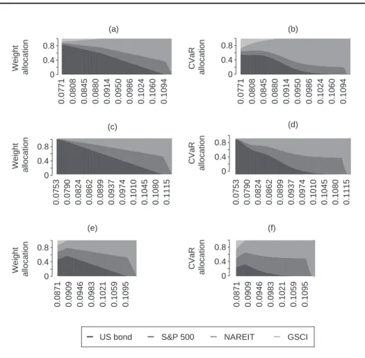
Asset allocation with conditional value-at-risk budgets 51 FIGURE 2 Weight and CVaR allocation of mean–standard deviation, mean–CVaR and mean–CVaR concentration efficient portfolios for various levels of annualized portfolio returns. 0.0771 0.0808 0.0845 0.0880 0.0914 0.0950 0.0986 0.1024 0.1060 0.1094 Weight allocation 0 0.4 0.8 0.0753 0.0790 0.0824 0.0862 0.0899 0.0937 0.0974 0.1010 0.1045 0.1080 0.1115 0.0871 0.0909 0.0946 0.0983 0.1021 0.1059 0.1095 CVaR allocation 0.0771 0.0808 0.0845 0.0880 0.0914 0.0950 0.0986 0.1024 0.1060 0.1094 0 0.4 0.8 0 0.4 0.8 0 0.4 0.8 0 0.4 0.8 0 0.4 0.8 0.0753 0.0790 0.0824 0.0862 0.0899 0.0937 0.0974 0.1010 0.1045 0.1080 0.1115 0.0871 0.0909 0.0946 0.0983 0.1021 0.1059 0.1095 Weight allocation Weight allocation CVaR allocation CVaR allocation (a) (b) (c) (d) (e) (f)
US bond S&P 500 NAREIT GSCI
(a), (b) Mean standard deviation. (c), (d) Mean–CVaR. (e), (f) Mean–CVaR concentration.
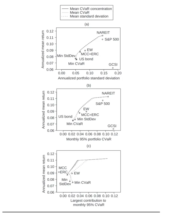
deviation and mean–CVaR efficient portfolios. Part (a) of Figure 3 plots the mean-risk frontiers, while part (c) shows the annualized mean return of the portfolios against the largest percentage CVaR contribution. A joint reading of these plots is needed to understand the trade-off between the maximum return, minimum risk and minimum risk concentration objectives.
The optimal weights for the mean–CVaR concentration portfolios as a function of the return target are reported in part (e) of Figure 2. Without return constraint, the MCC portfolio invests 47.34% in the bond index, 20.70% in the S&P 500 index, 18.44% in the NAREIT index and 13.52% in the GSCI. Part (f) of Figure 2 shows that the CVaR
allocation of the unconstrained MCC portfolio is very close to that of an equal risk contribution portfolio. Parts (a) and (b) of Figure 2 show the weight and CVaR allo-cation of the classical mean–standard deviation and mean–CVaR efficient portfolios. There are several striking differences. First, the mean–standard deviation portfolio is slightly more diversified than the mean–CVaR portfolio: 97% of the unconstrained min CVaR portfolio is invested in the bond index, against 84% for the minimum stan-dard deviation portfolio. Second, since the CVaR of the GSCI is significantly higher than the CVaR of the other asset class indexes, its percentage risk contribution is triple its portfolio weight. Third, the annualized returns of the minimum standard deviation and CVaR portfolios are 7.7% and 7.5%, respectively, while for the MCC portfolio it is 8.7%. The risk–return trade-off is visualized in Figure 3 on the facing page. We see that the equal-weight portfolio has the highest average return and risk of all uncon-strained portfolios, followed by the MCC portfolio. The risk–return characteristics of the min standard deviation and min CVaR portfolios are similar.
Figure 2 on the preceding page shows that imposing a return constraint on the minimum standard deviation and CVaR portfolios leads to a higher allocation to the S&P 500 and the NAREIT index, and a reduction in the bond and GSCI investment. Of course this leads to portfolios with a higher return and risk, but, interestingly, as long as the return target is below 9%, it reduces the risk concentration of the portfolio, as can be seen from part (c) of Figure 3 on the facing page. From that point onward, the NAREIT index becomes the largest risk contributor, and higher returns are traded off with both a higher total portfolio risk and risk concentration.
The mean–CVaR concentration efficient portfolio is very different from the mean– CVaR and mean–standard deviation efficient portfolios. On this data set, the mean– CVaR concentration efficient frontier has three distinct segments. Unconstrained, the mean–CVaR concentration efficient frontier is an equal risk contribution portfolio with an annualized return of 8.7%. For a target return between 8.7% and 9.01%, the portfolio CVaR concentration increases from 0.96% to 1.19%, but the portfolio CVaR decreases from 3.87% to 3.59%. This is due to a reallocation of the more risky commodity investment into bonds, equity and real estate, as can be seen in Figure 2 on the preceding page. At the end of this segment, only 1% of the portfolio is invested in commodities. Bonds dominate the portfolio budget allocation, with a 58% share. On the second segment, the bond allocation shrinks to zero, while the shares of the S&P 500 and the NAREIT index rise from 22% to 52% and from 20% to 48%, respectively. On this angle portfolio, the S&P 500 and NAREIT index each contribute 50% to the portfolio CVaR, which is now 7.0% compensated by a target return of 11%. The portfolios on the final segment of the frontier gradually replace the S&P 500 investment with the NAREIT. Since this asset offers the highest return, it is also the endpoint of the long-only constrained mean–CVaR concentration efficient frontier.
Asset allocation with conditional value-at-risk budgets 53 FIGURE 3 Annualized mean return versus the annualized portfolio standard deviation, the monthly portfolio 95% CVaR and the largest percentage CVaR contribution for the mean– standard deviation, mean–CVaR and mean–CVaR concentration efficient portfolios.
0.00 0.05 0.10 0.15 0.20 0.06 0.07 0.08 0.09 0.10 0.11 0.12
Annualized portfolio standard deviation
Annualized mean return
S&P 500 NAREIT EW MCC=ERC Min CVaR Min StdDev
Mean CVaR concentration Mean CVaR
Mean standard devation
0.00 0.02 0.04 0.06 0.08 0.10 0.12 0.06 0.07 0.08 0.09 0.10 0.11 0.12
Monthly 95% portfolio CVaR
0.00 0.02 0.04 0.06 0.08 0.10 0.12 0.06 0.07 0.08 0.09 0.10 0.11 0.12 Largest contribution to monthly 95% CVaR GCSI
Annualized mean return
Annualized mean return
(a) (b) (c) US bond MCC=ERC MCC =ERC EW EW Min StdDev Min StdDev Min CVaR Min CVaR NAREIT S&P 500 US bond GCSI
4.3 Dynamic investment strategies
Under a static risk budget allocation approach, the portfolio manager has determined a desired asset allocation and does not intend to stray far from it. However, it is well-known that the risk and dependence of most financial assets are time-varying, which means that the optimal risk budget allocation portfolios also change over time.
Let us therefore consider a dynamic portfolio invested in bonds, equity, real estate and commodities. The portfolio is rebalanced quarterly to satisfy an equal-weight, minimum CVaR or MCC objective. The CVaR budgets are computed by the Cornish–Fisher method in Boudtet al(2008), requiring an estimate of the first four (co)moments of the multivariate return distribution. Estimation of these moments is conditional on the information available at the time of rebalancing, as detailed in Appendix A.
Since we required a minimum sample size of eight years and the data span is Jan-uary 1976–June 2010, the optimized weights are available for the quarters 1984 Q1– 2010 Q3. First, we discuss the results for the equal-weight, minimum CVaR and MCC portfolios. Second, we analyze the sensitivity of the minimum CVaR and MCC port-folios to the inclusion of a weight or risk allocation constraint and the choice of risk measure.1
4.3.1 Results for unconstrained portfolios
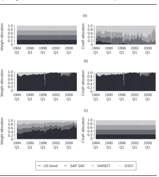
Figure 4 on the facing page plots the weight and CVaR allocations of the equal-weight, minimum CVaR, and MCC portfolios. We find that, for almost all periods, the mini-mum CVaR portfolio is highly invested in the bond index, while the MCC portfolio is more balanced across all asset classes. As predicted by the theory, the risk allocation of the minimum CVaR portfolio coincides with its weight allocation. The risk alloca-tion of the MCC portfolio is almost identical to the equal risk contribualloca-tion state. The CVaR of the equal-weight portfolio is dominated by the S&P 500, GSCI and NAREIT indexes, while the risk contribution of the bond is almost zero for many quarters. The reason for the bad performance of weight constraints in ensuringex anterisk diversi-fication is the nonlinear dependence of portfolio CVaR contributions on the weights. Reaching the portfolio manager’s goal of ensuring risk diversification is therefore more efficiently achieved via direct constraints on the risk budget contributions rather than the weights.
1As noted by a referee, even though we evaluate the portfolios based on their performance, none of the objectives considered include performance (absolute or risk-adjusted). This is because of the difficulty in forecasting properly expected return, compared with forecasting risk, as already mentioned by Merton (1980).
Asset allocation with conditional value-at-risk budgets 55 FIGURE 4 Stacked bar weight and CVaR contribution plots for the quarterly rebalanced equal-weight, minimum CVaR and minimum CVaR concentration portfolios.
1984 Q1 1990 Q1 1996 Q1 2002 Q1 2008 Q1 (a) Weight allocation 0 0.2 0.4 0.6 0.8 1.0 (b) CVaR allocation 1984 Q1 1990 Q1 1996 Q1 2002 Q1 2008 Q1 1984 Q1 1990 Q1 1996 Q1 2002 Q1 2008 Q1 1984 Q1 1990 Q1 1996 Q1 2002 Q1 2008 Q1 1984 Q1 1990 Q1 1996 Q1 2002 Q1 2008 Q1 1984 Q1 1990 Q1 1996 Q1 2002 Q1 2008 Q1 0 0.2 0.4 0.6 0.8 1.0 0 0.2 0.4 0.6 0.8 1.0 0 0.2 0.4 0.6 0.8 1.0 0 0.2 0.4 0.6 0.8 1.0 0 0.2 0.4 0.6 0.8 1.0 Weight allocation
Weight allocation CVaR allocation
CVaR allocation
(c)
US bond S&P 500 NAREIT GSCI
(a) Equal weight. (b) Minimum CVaR. (c) Minimum CVaR concentration.
Part (a) in Figure 5 on the next page plots theex anteportfolio risk estimates. As expected, the CVaR of the MCC portfolio is for all quarters in between the CVaR of the minimum CVaR portfolio and the CVaR of the equal-weight portfolio.
The solid gray and black lines in part (b) of Figure 5 on the next page plot the ratio of the monthly cumulative out-of-sample returns of the minimum CVaR and MCC portfolios versus the cumulative returns of the equal-weight portfolio over the period January 1984–June 2010. The value of the chart is less important than the slope of the
FIGURE 5 Monthly CVaR of (a) the quarterly rebalanced equal-weight, minimum CVaR and minimum CVaR concentration portfolios and (b) the relative performance of the quar-terly rebalanced minimum CVaR and minimum CVaR concentration portfolios versus the equal-weight portfolio. Jan 1984 Jan 1987 Jan 1990 Jan 1993 Jan 1996 Jan 1999 Jan 2002 Jan 2005 Jan 2008 Jun 2010 Portfolio CVaR Equal weight
Min CVaR concentration Min CVaR
Relative performance
vs. equal weight
Min CVaR concentration Min CVaR Jan 1984 Jan 1987 Jan 1990 Jan 1993 Jan 1996 Jan 1999 Jan 2002 Jan 2005 Jan 2008 Jun 2010 0 0.5 0.15 0.10 1.2 0.8 1.6 1.0 1.4 (b) (a)
The shaded regions indicate a bear market regime.
line. If the slope is positive, the strategy in the numerator is outperforming the equal-weight strategy, and vice versa. The vertical gray bars denote bear markets, defined by Ellis (2005) as periods with a decline in the S&P 500 index of 12% or more. The left-hand side of the bar corresponds to the market peaks and the right-hand side to the stock market trough. We see in Figure 5 that the minimum CVaR portfolio, having a large allocation to bonds, outperforms the equal-weight and MCC portfolios at times of serious stock market downturn. The performance of the MCC portfolio seems to be a middle ground between the performance of the equal-weight and minimum CVaR portfolios. It offers an attractive compromise between the good performance of the
Asset allocation with conditional value-at-risk budgets 57
minimum CVaR portfolio in adverse markets and the upward potential of the equal-weight portfolio. A final observation is that periods where one strategy outperforms the other are relatively long and indicate the possibility of applying market timing strategies on top of these allocations.
Table 2 on the next page reports the annualized out-of-sample average return on the portfolios. When computed over the whole period, the minimum CVaR and MCC portfolios performed within 15 bps of one another. This is a small margin, given the long period of time presented. The risk statistics computed from the out-of-sample returns confirm the ex anterisk estimates from Figure 5 on the facing page. The value of the annualized standard deviation and monthly historical CVaR of the MCC portfolio is in between those of the minimum CVaR portfolio and the equal-weight portfolio. In the credit crisis the equal-weight portfolio suffered a drawdown of 52%, which is significantly higher than the 34% drawdown of the MCC portfolio.
Splitting the sample into bull/bear periods, we see a much bigger variation in relative performance. The (annualized) return for the minimum CVaR portfolio trailed the MCC portfolio by more than 300 bps during equity bull markets, yet outperformed during bear markets by more than 1800 bps. The minimum CVaR and MCC portfolio therefore both have their appeal, depending on the market environment. This might lead to risk timing the portfolio allocation, whereby the investor selects their risk appetite based on broad market conditions. In a secular bull market, the investor might choose the MCC portfolio because of its relative outperformance in exchange for the risk of slightly larger losses. In a secular bear market, the minimum CVaR portfolio might be more appealing because of its conservatism.
Recall from (3.6) that the MCC portfolio is designed to have both a low downside risk and high downside risk diversification. To verify that the MCC effectively retains this property out-of-sample, we report in Table 2 on the next page the average Gini coefficient of the portfolio weights and the historical CVaR percentage concentration. The Gini coefficient takes values between 0 (equal-weight portfolio) and 1 (portfolio concentrated on one asset).2 We see that the minimum CVaR portfolio is heavily concentrated on a few assets compared with the MCC portfolio. The MCC portfolio thus strikes an attractive balance between a high risk adjusted return performance and a well-diversified portfolio. The historical CVaR percentage concentration is computed as the average proportion between the largest component loss contribution and the total loss for all losses that exceed the 5% quantile loss, computed using the returns from inception. We see that the equal-weight portfolio has the lowest CVaR percentage concentration, but the highest CVaR. In contrast, the minimum CVaR portfolio has 2The Gini index is a measure of dispersion using the Lorenz curve. Letzbe a random variable onŒ0; 1with distribution function F. The Gini index is calculated as12R01L.z/dz, where L.z/DR0zudF .u/=R01udF .u/.
K.
Boudt
et
al
TABLE 2 Summary statistics of monthly out-of-sample returns on equal-weight, minimum portfolio CVaR (concentration) investment strategies over the period January 1984–June 2010. [Table continues on next page.]
Objective
‚ …„ ƒ
Min CVaR
‚ …„ ƒ Min CVaR
40% 40% CVaR conc.
Equal Min Min CVaR position allocation 40% position
Constraint weight CVaR conc. limit limit ERC limit
(a) Full period (%)
Annual mean 7.11 7.55 7.40 7.40 7.44 7.40 7.33
Annual SD 10.06 4.72 7.42 8.52 6.61 7.42 8.42
Skewness 3.14 0.49 2.35 2.36 1.92 2.35 2.69
Excess kurtosis 23.42 3.62 15.11 14.59 11.12 15.10 18.37
Monthly historical CVaR 7.55 2.62 5.14 6.17 4.51 5.14 6.08
Gini portfolio weights 0.00 0.68 0.25 0.23 0.47 0.25 0.17
Monthly historical CVaR 0.63 0.96 0.62 0.71 0.76 0.62 0.61
% concentration
Portfolio turnover 5.01 10.31 9.04 11.30 12.45 9.04 8.07
(b) Normal/bull stock market (%)
Annual mean 12.64 8.02 11.33 12.19 10.42 11.33 11.96
Annual SD 7.06 4.40 5.71 6.40 5.28 5.71 6.20
Skewness 0.30 0.12 0.13 0.26 0.08 0.13 0.23
Excess kurtosis 0.84 1.57 0.39 1.10 1.18 0.39 0.74
Monthly historical CVaR 3.51 2.07 2.65 3.06 2.42 2.65 3.00
Jour nal of Risk V olume 15/Number 3, Spr ing 2013
Asset allocation with conditional v alue-at-r isk b udgets 59 TABLE 2 Continued. Objective ‚ …„ ƒ Min CVaR ‚ …„ ƒ Min CVaR 40% 40% CVaR conc.
Equal Min Min CVaR position allocation 40% position
Constraint weight CVaR conc. limit limit ERC limit
(c) Bear stock market (%)
Annual mean 21.83 5.10 13.18 17.64 8.14 13.19 16.93
Annual SD 17.10 6.14 11.52 13.37 10.18 11.53 13.60
Skewness 2.59 1.46 2.56 2.30 2.18 2.56 2.54
Excess kurtosis 9.65 4.33 8.40 7.18 5.93 8.40 8.82
Monthly historical CVaR 15.44 4.31 11.06 12.63 9.57 11.06 12.80
(d) Drawdowns higher than 10%
Credit crisis1 0.52 0.10 0.34 0.41 0.27 0.34 0.42
Asian–Russian 0.15 0.11 0.10 0.11
crisis2
Black Monday3 0.11 0.11 0.11 0.11 0.11
1May 2008–February 2008 for the min CVaR portfolio, November 2007–February 2009 for the min CVaR portfolio with position or risk allocation limit, otherwise June 2008–February 2009.2October 1997–August 1998 for the equal-weight portfolio, otherwise April–August 1998.3August–November 1987 for the equal-weight portfolio, otherwise August–October 1987. Research P aper www .r isk.net/jour nal
the lowest CVaR, but the highest CVaR percentage concentration. The MCC portfolio combines both a low CVaR concentration and low total portfolio CVaR.
Finally, we consider the portfolio turnover of the strategies, defined by DeMiguel
et al (2009) as the average sum of the absolute value of the trades across the N
available assets: turnoverD 1 T1 TX1 tD1 N X iD1 jw.i /tC1w.i /tCj; (4.1)
wherew.i /tC1is the weight of assetiat the start of rebalancing periodtC1,w.i /tCis the weight of that asset before rebalancing attC1andTis the total number of rebal-ancing periods. This turnover quantity can be interpreted as the average percentage of wealth traded in each period. The portfolio turnover is the lowest for the equal-weight portfolio (5.01%). The MCC portfolio has a significantly lower turnover (9.04%) than the minimum CVaR portfolio (10.31%).
In conclusion, over the period January 1984–June 2010, the minimum CVaR port-folio has the lowest out-of-sample risk but a high risk concentration and turnover. The equal-weight strategy has the lowest turnover and risk concentration, but high-est total risk. The proposed MCC portfolio is the second bhigh-est in all these aspects. It achieves an attractive compromise between low overall risk, good upside return, high diversification and low turnover. When we condition on the market regime, we find that in bear markets, as expected, the minimum CVaR portfolio outperforms all strategies, but has a lower return in normal/bull markets than the equal-weight and MCC portfolios. Compared with the equal-weight diversification strategy, the MCC portfolio has a comparable return but lower risk in a normal/bull stock market, and its performance is less affected when the market regime switches to a more negative outlook. For this reason, we recommend a minimum CVaR allocation strategy in a bear market regime and the MCC strategy in a normal/bull market regime.
4.3.2 Sensitivity to weight and CVaR allocation constraints
The MCC portfolio directly optimizes the risk diversification of the portfolio. Previous research by Maillardet al (2010), Qian (2005) and Zhuet al(2010), however, has focused on using risk budgets as a constraint in the portfolio allocation, or imposing diversification through weight constraints. In Table 3 on the facing page, Figure 6 on page 62 and Figure 7 on page 63, we investigate the sensitivity of the portfolios to an equal risk contribution constraint, an upper 40% position limit or an upper 40% CVaR allocation limit. The choice of 40% is arbitrary, but it is consistent with the 40% allocation to equity in the stylized 60/40 bond–equity portfolio.
Part (a) of Figure 6 on page 62 presents the weight allocations of the constrained minimum CVaR portfolios. We see that the 40% upper bound on the portfolio weights
Asset allocation with conditional value-at-risk budgets 61 TABLE 3 Summary statistics of monthly out-of-sample returns on minimum portfolio
standard deviation (concentration) investment strategies over the period January 1984– June 2010.
Objective
‚ …„ ƒ
Min SD Min SD
Min SD ‚ …„ ƒ conc.
Min conc. 40% SD allocation 40% pos
Constraint SD 40% pos limit limit ERC limit
(a) Full period (%)
Annual mean 7.48 7.30 6.96 7.21 7.30 7.17
Annual SD 4.62 7.02 8.18 6.13 7.02 8.22
Skewness 0.42 2.48 2.50 1.73 2.48 2.89
Excess kurtosis 1.86 17.20 16.99 10.55 17.19 21.36
Monthly historical CVaR 2.37 4.82 5.80 3.85 4.82 5.93
Gini portfolio 0.62 0.28 0.28 0.46 0.28 0.18
weights
Monthly historical CVaR 0.90 0.64 0.65 0.76 0.64 0.61 % conc
Portfolio turnover 11.79 8.63 14.90 12.97 8.64 7.61
(b) Normal/bull stock market (%)
Annual mean 7.99 10.66 10.57 9.10 10.67 11.35
Annual SD 4.39 5.45 6.41 5.27 5.46 6.08
Skewness 0.05 0.20 0.39 0.27 0.20 0.27
Excess kurtosis 0.34 0.22 0.98 0.07 0.22 0.66
Monthly historical CVaR 2.02 2.52 3.17 2.61 2.52 2.93 (c) Bear stock market (%)
Annual mean 4.83 10.32 11.94 2.71 10.33 14.71
Annual SD 5.63 11.07 13.01 8.96 11.07 13.56
Skewness 1.16 2.70 2.63 2.52 2.70 2.71
Excess kurtosis 3.46 10.11 9.78 9.78 10.10 10.40
Monthly historical CVaR 3.51 9.97 12.08 7.64 9.97 12.53 (d) Drawdowns higher than 10%
Credit crisis1 0.33 0.41 0.25 0.33 0.42
Asian–Russian 0.11 0.17 0.14 0.11 0.12
crisis2
1June 2008–February 2009.2November 1997–August 1998 for the minimum standard deviation concentration and
ERC constrained portfolios. Otherwise November 1997–February 1998.
FIGURE 6 Stacked bar weight and CVaR contribution plots for the constrained minimum CVaR and minimum CVaR concentration portfolios invested in the Merrill Lynch US bond, S&P 500, NAREIT and S&P GSCI indexes.
0 0.4 0.8 Weight allocation Weight allocation Weight allocation CVaR allocation CVaR allocation CVaR allocation 1984 Q1 1990 Q1 1996 Q1 2002 Q1 2008 Q1 1984 Q1 1990 Q1 1996 Q1 2002 Q1 2008 Q1 1984 Q1 1990 Q1 1996 Q1 2002 Q1 2008 Q1 1984 Q1 1990 Q1 1996 Q1 2002 Q1 2008 Q1 1984 Q1 1990 Q1 1996 Q1 2002 Q1 2008 Q1 1984 Q1 1990 Q1 1996 Q1 2002 Q1 2008 Q1 0 0.4 0.8 0 0.4 0.8 0 0.4 0.8 0 0.4 0.8 0 0.4 0.8 (a) (c) (b)
US bond S&P 500 NAREIT GSCI
The portfolios are rebalanced quarterly. (a) Min CVaR + 40% position limit. (b) Min CVaR + 40% CVaR allocation limit. (c) Min CVaR concentration + 40% position limit.
and risk allocations is stringent for almost all periods. Under these constraints, the component CVaR contribution of the minimum CVaR portfolio no longer coincides with the weight allocation. The investment in the bond typically contributes less to CVaR risk than its portfolio weight. Its contribution is for some months even negative under the position limit. Part (c) of Figure 6 shows the weight and risk allocation of the MCC portfolio under a 40% upper bound on the portfolio weights. We see that, in spite of the weight constraint, the risk of the MCC portfolio is still more equally spread out than for the minimum CVaR portfolio, where for some periods the S&P 500 investment causes more than half of portfolio risk.
Asset allocation with conditional value-at-risk budgets 63 FIGURE 7 Monthly CVaR of (a) the quarterly rebalanced constrained minimum CVaR and minimum CVaR concentration portfolios and (b) the relative performance of the quar-terly rebalanced constrained minimum CVaR and minimum CVaR concentration portfolios versus the equal-weight portfolio.
0 Portfolio CVaR Relative performance vs equal weight 0.10 0.05 0.15 0.8 1.0 1.2 1.4 1.6 Jan 1984 Jan 1987 Jan 1990 Jan 1993 Jan 1996 Jan 1999 Jan 2002 Jan 2005 Jan 2008 Jun 2010 Jan 1984 Jan 1987 Jan 1990 Jan 1993 Jan 1996 Jan 1999 Jan 2002 Jan 2005 Jan 2008 Jun 2010 (b) (a)
Min CVaR + 40% CVaR alloc limit
Min CVaR concentration +40% position limit Min CVaR + 40% position limit
Min CVaR + ERC constraint
The shaded regions indicate a bear market regime.
From the weight and CVaR allocation plots, it is clear that adding position or risk allocation limits pushes the minimum CVaR and MCC portfolio toward an allocation that is closer to the equal-weight portfolio. Consequently, the return, risk and turnover properties of these constrained portfolios are closer to the equal-weight portfolio, as can be seen in Table 3 on page 61 and Figure 7. Compared with the 40% CVaR
tion limit, the maximum 40% weight constraint leads to portfolios with a substantially higher predicted risk (see part (a) of Figure 6 on page 62) and realized risk (see the standard deviation and historical CVaR values in Table 3 on page 61). In all aspects, the unconstrained MCC portfolio and ERC constrained minimum CVaR portfolios are very similar.
4.3.3 Sensitivity to the choice of risk measure
In Maillardet al (2010), Qian (2005) and Zhuet al(2010), the portfolio standard deviation is used as the risk measure in the risk allocation portfolio. We analyze the sensitivity of our results to the use of downside risk measures in Table 3 on page 61, where we report the performance statistics for the same investment styles, but using the portfolio standard deviation as the risk measure. Overall, it seems that, for this investment universe, changing the risk measure only has a marginal impact on the out-of-sample performance, compared with the choice of investment style. In fact, when testing for the equality of the Sharpe ratios between the minimum CVaR (concentration) and minimum standard deviation (concentration) portfolios using the test of Jobson and Korkie (1981) and Memmel (2003), we do not find a significant difference in performance at a 90% confidence level. Similarly to the CVaR risk measure, we find that the minimum standard deviation concentration portfolio constitutes an attractive middle ground between the upward potential of the equal-weight portfolio in normal/bull markets and the low risk of the minimum standard deviation portfolio.
5 CONCLUSION
An extensive empirical application of ex ante downside risk budget methods to dynamic allocation across bonds, commodities, domestic and international equity illustrated the out-of-sample effectiveness of downside risk budgets in generating portfolios that have low portfolio risk and risk concentration, high diversification and low portfolio turnover. A first strategy is to impose bound constraints on the percent-age CVaR contributions. This provides a direct substitute and improvement to the commonly practiced risk diversification approach based on position limits. A sec-ond strategy consists of minimizing the largest component CVaR contribution, which directly addresses risk diversification, even in portfolios with nonnormally distributed assets. The properties of these approaches as described in this paper compare favor-ably to the equal-weight portfolio. Unconstrained, the minimum CVaR concentration portfolio is typically similar to the equal risk contribution portfolio of Qian (2005). Furthermore, it may be easily combined with many other investor objectives and con-straints (such as return targets or drawdown and cardinality concon-straints). Investors can thus optimally balance their maximum return, minimum downside risk and maximum
Asset allocation with conditional value-at-risk budgets 65
downside risk diversification objectives through anex anteuse of CVaR budgets in portfolio optimization. Based on our empirical study, we recommend the optimiza-tion of the asset allocaoptimiza-tion according to a minimum CVaR objective in a bear market regime and the minimization of the portfolio’s CVaR concentration in a normal/bull market regime.
There are several interesting directions for further research. First of all, the risk allocation methodology could be applied to a large-scale equity portfolio, in which case we recommend the formulation of the risk budget constraints and objectives at a more aggregate level, such as at the level of the country and industry rather than the individual stock. A second topic for further research is the choice of downside risk estimator and the loss probability at which the downside risk is computed. Finally, a switching allocation rule between a low-risk strategy and a strategy that combines risk objectives with views on the returns also merits further research.
APPENDIX A
A.1 CVaR budget of the fully invested minimum CVaR portfolio The Langrangian associated with the fully invested minimum CVaR portfolio is
CVaRw.˛/C.w01/; (A.1)
withtheN1vector with each element equal to 1. From the first order conditions, it follows that @CVaRw.˛/ @w ˇ ˇ ˇ
ˇwDwmin CVaRD : (A.2)
Hence, the partial derivatives should all be equal, and because
C.i /CVaRw.˛/Dw.i /
@CVaRw.˛/ @w.i /
;
there exists a unique constantksuch that
w.i /min CVaR DkC.i /CVaRwmin CVaR.˛/; (A.3) for alli D1; : : : ; N. Because of the full investment constraint, the weights need to sum up to unity, which is satisfied fork D 1=CVaRwmin CVaR.˛/. Replacingk with
1=CVaRwmin CVaR.˛/in (A.3) yields that the weight and percentage CVaR allocation coincide for the minimum CVaR portfolio.
A.2 Implementation of the CVaR estimator
The CVaR estimator requires an estimate of theN1conditional meant, theNN
conditional covariance matrix˙t, theN N2conditional coskewnesst, and the
NN3cokurtosis matrix t. We obtain estimates of these conditional (co)moments
through the following stepwise estimation procedure.
(1) Estimate the conditional mean monthly returntas the sample average of the
returns from inception up to montht1.
(2) Center the monthly returns in the sample around t: rNs D rs t for all sD1; : : : ; t1.
(3) Estimate the conditional covariance matrix for each return in the sample, as well as the conditional covariance matrix for next month’s return (˙t), using
the DCC–GARCH(1,1) model of Engle (2002). Under this approach, the param-eters of the individual GARCH(1,1) volatilities and conditional correlations are estimated separately, using a two-stage quasi-maximum likelihood estimation procedure with variance and correlation targeting. The conditional covariances are then computed as products of individual volatilities and conditional corre-lations.
(4) For the returns in the sample, compute the devolatilized centered return series:
us DPs1=2rNsfor allsD1; : : : ; t1.
(5) Use the Winsorization procedure of Boudtet al(2008) to reduce the magnitude of the most extreme devolatilized return vectors in the sample.
(6) Compute the equicorrelation estimator oft and t on the sample of
Win-sorized devolatilized returns, as proposed by Martellini and Ziemann (2010). Given a portfolio weight vectorw, the second, third and fourth portfolio moments can then be computed as
m2t Dw0˙tw; m3t Dw0t.w˝w/; m4t Dw0 t.w˝w˝w/;
respectively, where˝denotes the Kronecker product. The portfolio skewnessst D m3t=m3=22t and the excess kurtosiskt Dm4t=m22t3.
The Cornish–Fisher-based CVaR estimator proposed by Boudt et al (2008) is derived from the Cornish–Fisher expansion. For a zero mean, unit variance random variable with skewnessst and excess kurtosiskt, the second order Cornish–Fisher
expansion of the quantile function around the Gaussian quantile function ˚1./
equals
g˛t Dz˛C 16.z˛21/stC 241.z˛33z˛/kt 361.2z˛35z˛/s2t; (A.4)
withz˛ D˚1.˛/. The Cornish–Fisher CVaR for the portfolio return in montht is
then given by
CVaRt.˛/D w0tC
p
Asset allocation with conditional value-at-risk budgets 67 with dt.˛/D 1 ˛f.g˛t/C 1 24ŒI 4 6I2C3.g˛t/ktC16ŒI33I1st
C721 ŒI615I4C45I215.g˛t/sp2g
and where Iq D 8 ˆ ˆ ˆ ˆ ˆ < ˆ ˆ ˆ ˆ ˆ : q=2 X iD1 Qq=2 jD12j Qi jD12j g2i˛t.g˛t/C q=2 Y jD1 2j .g˛t/ forqeven; q X iD0 Qq jD0.2jC1/ Qi jD0.2jC1/ g2i˛tC1.g˛t/ q Y jD0 .2jC1/ ˚.g˛t/ forqodd;
q D .q1/=2and./and˚./are the standard normal density and cumulative distribution functions, respectively.
Although the CVaR estimation formulas seem rather complex, they lend them-selves to efficient translation into a simple algorithm that computes both CVaR and component CVaR in less than a second, even for portfolios with a large number of assets.3
REFERENCES
Ardia, D., Boudt, K., Carl, P., Mullen, K., and Peterson, B. (2011). Differential evolution (DEoptim) for non-convex portfolio optimization. R Journal 3(1), 27–34.
Artzner, P., Delbaen, F., Eber, J. M., and Heath, D. (1999). Coherent measures of risk.
Mathematical Finance 9(3), 203–228.
Boudt, K., Peterson, B. G., and Croux, C. (2008). Estimation and decomposition of downside risk for portfolios with non-normal returns. The Journal of Risk 11(2), 79–103.
Boudt, K., Carl, P., and Peterson, B. G. (2011). PortfolioAnalytics: portfolio analysis, includ-ing numeric methods for optimization of portfolios. R Package, Version 0.6.1.
Carl, P., and Peterson, B. G. (2010). PerformanceAnalytics: econometric tools for perfor-mance and risk analysis. R Package, Version 1.0.2.1.
Choueifaty, Y., and Coignard, Y. (2008).Toward maximum diversification. Journal of Portfolio
Management 35(1), 10–24.
Chow, G., and Kritzman, M. (2001). Risk budgets. Journal of Portfolio Management 27(2), 56–60.
DeMiguel, V., Garlappi, L., and Uppal, R. (2009). Optimal versus naïve diversification: how inefficient is the1=N portfolio strategy? Review of Financial Studies 22(5), 1915–1953. Denault, M. (2001). Coherent allocation of risk capital. The Journal of Risk 4(1), 1–33. Ellis, J. (2005). Ahead of the Curve: A Commonsense Guide to Forecasting Business and
Market Cycles. Harvard Business Press, Cambridge, MA.
3The estimator is available in Carl and Peterson’s (2010) R package PerformanceAnalytics.
Engle, R. (2002). Dynamic conditional correlation: a simple class of multivariate gener-alised autoregressive conditional heteroskedasticity models. Journal of Business and
Economic Statistics 20(3), 339–350.
Jobson, J., and Korkie, B. (1981). Performance hypothesis testing with the Sharpe and Treynor measures. Journal of Finance 36(4), 889–908.
Keel, S., and Ardia, D. (2011). Generalized marginal risk. Journal of Asset Management 12(2), 123–131.
Lee, W. (2011). Risk-based asset allocation: a new answer to an old question? Journal of
Portfolio Management 37(4), 11–28.
Litterman, R. B. (1996). Hot spotsTMand hedges. Journal of Portfolio Management 22(5), 52–75.
Maillard, S., Roncalli, T., and Teiletche, J. (2010). On the properties of equally-weighted risk contributions portfolios. Journal of Portfolio Management 36(4), 60–70.
Martellini, L., and Ziemann, V. (2010). Improved forecasts of higher-order comoments and implications for portfolio selection. Review of Financial Studies 23(4), 1467–1502. Memmel, C. (2003). Performance hypothesis testing with the Sharpe ratio. Finance Letters
1(1), 21–23.
Merton, R. (1980). On estimating the expected return on the market. Journal of Financial
Economics 8(4), 323–361.
Pearson, N. D. (2002). Risk Budgeting: Portfolio Problem Solving with Value-at-Risk, 1st edn. Wiley.
Peterson, B. G., and Boudt, K. (2008). Component VAR for a non-normal world. Risk 21(11), 78–81.
Pflug, G. C. (2000). Some remarks on the value-at-risk and the conditional value-at-risk. In
Probabilistic Constrained Optimization: Methodology and Applications, Uryasev, S. (ed),
pp. 272–281. Kluwer, Dordrecht.
Price, K., Storn, R., and Lampinen, J. (2005). Differential Evolution: A Practical Approach
to Global Optimization. Springer.
Qian, E. (2005). Risk parity portfolios: efficient portfolios through true diversification of risk. Report, Panagora Asset Management (September).
Rockafellar, R. T., and Uryasev, S. (2000). Optimization of conditional value-at-risk. The
Journal of Risk 2(3), 21–41.
Scaillet, O. (2002). Nonparametric estimation and sensitivity analysis of expected shortfall.
Mathematical Finance 14(1), 74–86.
Scherer, B. (2007). Portfolio Construction and Risk Budgeting, 3rd edn. Risk Books, Lon-don.
Stoyanov, S., Rachev, S. T., and Fabozzi, F. J. (2009). Sensitivity of portfolio VaR and CVaR to portfolio return characteristics. Working Paper, Universität Karlsruhe.
Topaloglou, N., Vladimirou, H., and Zenios, S. A. (2002). CVaR models with selective hedg-ing for international asset allocation. Journal of Bankhedg-ing and Finance 26(7), 1535–1561. Zhu, S., Li, D., and Sun, X. (2010). Portfolio selection with marginal risk control. The Journal