BuildingIQ Technology Field Validation

(1)

Lawrence Berkeley National Laboratory

Recent Work

Title

BuildingIQ Technology Field Validation Permalink https://escholarship.org/uc/item/496616b6 Authors Granderson, Jessica Lin, Guanjing Singla, Rupam et al. Publication Date 2019-01-23 DOI 10.20357/B70W2P Peer reviewed

eScholarship.org Powered by the California Digital Library

(2)

DOI: 10.20357/B70W2P

BuildingIQ Technology Field Validation

Jessica Granderson

Guanjing Lin

Rupam Singla

Samuel Fernandes

Samir Touzani

Energy Technologies Area

November 2018

(3)

DISCLAIMER

This document was prepared as an account of work sponsored by the United States Government. While this document is believed to contain correct information, neither the United States Government nor any agency thereof, nor The Regents of the University of California, nor any of their employees, makes any warranty, express or implied, or assumes any legal responsibility for the accuracy, completeness, or usefulness of any information, apparatus, product, or process disclosed, or represents that its use would not infringe privately owned rights. Reference herein to any specific commercial product, process, or service by its trade name, trademark, manufacturer, or otherwise, does not necessarily constitute or imply its endorsement, recommendation, or favoring by the United States Government or any agency thereof, or The Regents of the University of California. The views and opinions of authors expressed herein do not necessarily state or reflect those of the United States Government or any agency thereof or The Regents of the University of California.

ACKNOWLEDGEMENT

This work was supported by the Assistant Secretary for Energy Efficiency and Renewable Energy, Building Technologies Office, of the U.S. Department of Energy (DOE) under Contract No. DE-AC02-05CH11231. The authors thank each of the following for their contributions to this evaluation: Vincent Perrier, Department of General Services, Washington D.C.; Zach Wilson and Will Gee, New City Energy, Washington D.C.; Roberto Nunez, Jose Fernandez, and Jeffrey Hogan, New York-Presbyterian Allen Hospital; Tony Covarrubias and Michael Clemson, California State University, Long Beach; Courtney Hatchel, Scott Day and Eric Pierce, GSA Federal Courthouse Building, Dayton, Ohio; Cameron Kaminsky and Todd Kronlein, GSA IRS Annex, Chamblee Georgia; Michael Hobson and Kevin Powell, GSA; and Amy Jiron, DOE. Xiufeng Pang of Lawrence Berkeley National Laboratory provided valuable contributions to the site selection, metering, and monitoring of sites in the initial phases of this project.

(4)

iii

5. Discussion ... 26 6. Conclusions ... 28 References ... 29 Appendix A: BuildingIQ Site Selection Criteria ... A-1 Appendix B: Demonstration Site Characteristics ... B-1 Appendix C: Metering ... C-1 Appendix D: Baseline Model Fitness Metrics ... D-1 Appendix E: Space Air Relative Humidity Calculation Process ... E-1 Appendix F: Interview Questions for Site Points of Contact ... F-1 Appendix G: Baseline Model Used for the CSU Site ... G-1 Appendix H: Total, Monthly, and Seasonal Savings at the Chamblee Site ... H-1 Appendix I: Contrasting Example of AHU Static Pressure and Supply Air Temperature During PEO-On and PEO-Off Periods... I-1 Appendix J: Example of a Building Audit Report ... J-1

List of Tables

Table 1: Performance objectives of the BuildingIQ field verification ... 1 Table 2: Cohort of demonstration sites ... 4 Table 3: Data collected at each site to determine energy and utility cost savings ... 6 Table 4: Baseline model goodness-of-fit metrics for each site at the HVAC isolation level, for baseline data collected ... 11 Table 5: HVAC energy savings at each site ... 12 Table 6: Mechanical issues detected at Woodson High School ... 17 Table 7: The number of times that the change in space air temperature exceeded the maximum allowable during the studied time period, for each time duration in ASHRAE Standard 55 ... 19 Table 8: Hot and cold complaints record from sites ... 20 Table 9: Estimated cost savings and technology costs to meet a five-year payback ... 21 Table B-1: California State University, Long Beach ... B-1 Table B-2: GSA Dayton... B-1 Table B-3: New York-Presbyterian – Allen Hospital ... B-2 Table B-4: Washington, D.C., Woodson High School ... B-2 Table B-5: GSA Chamblee ... B-3 Table C-1: Specifications for CSU Long Beach Metering ... C-1

(6)

v

Table C-2: Specifications for GSA Dayton Metering... C-3 Table C-3: Specifications for New York-Presbyterian – Allen Hospital Metering ... C-4 Table C-4: Specifications for Woodson High School Metering ... C-6 Table C-5: Specifications for Chamblee IRS Annex Metering ... C-8

List of Figures

Figure ES-1: Time-averaged HVAC power comparison at four field evaluation sites; red indicates the baseline projected load for each hour of the day or day of the week, and blue

indicates the metered load under PEO-on controls. ... 3

Figure ES-2: Decrease in AHU static pressure and fan speed effected by PEO’s optimization strategy ... 4

Figure ES-3: Percentage of operational points outside of the comfort zone for each VAV zone, during the PEO-on (blue) and the PEO-off (red) time periods at two sites ... 4

Figure 1: Illustration of the BuildingIQ technology ... 2

Figure 2: BuildingIQ data flow ... 3

Figure 3: Optimized temperature control between upper and lower control limits ... 3

Figure 4: PEO dashboard showing trends of meter and BAS trend log data ... 6

Figure 5: A simplified representation of the ASHRAE thermal comfort model, with comfort as a function of relative humidity and air temperature ... 9

Figure 6: Daily power comparison for the HVAC system time averaged over the 12-month monitoring period at the CSU site ... 13

Figure 7: Decrease in AHU static pressure and fan speed at the CSU site (OAT stands for outside air temperature). ... 13

Figure 8: AHU supply air temperature comparison in PEO-on and PEO-off mode at the CSU site ... 14

Figure 9: Time-averaged HVAC power comparison at the Dayton (top left), NYP Allen (top right), and Woodson (bottom left) sites; red indicates the baseline projected load for each hour of the day, and blue indicates the metered load under PEO-on controls. ... 15

Figure 10: Percentage of operational points (space temperature paired with space humidity) outside of the comfort zone for each VAV, during the PEO-on (blue) and the PEO-off (red) time periods at Dayton Courthouse and Woodson High School ... 19

Figure 11: BuildingIQ implementation lead time ... 22

Figure 12: Screen capture of visualization capabilities in the BuildingIQ portal ... 25 Figure C-1: Electrical submetering locations for CSU Long Beach... C-2 Figure C-2: Electrical submetering locations for GSA Dayton ... C-3

(7)

vi

Figure C-3: Electrical submetering locations for New York-Presbyterian – Allen Hospital ... C-5 Figure C-4-1: Electrical submetering locations for Woodson High School – switchboard 1 .... C-7 Figure C-4-2: Electrical submetering locations for Woodson High School – switchboard 2 .... C-7 Figure C-5-1: Electrical submetering locations for Chamblee IRS Annex – Panel SSS, AHU . C-9 Figure 5-2: Electrical submetering locations for Chamblee IRS Annex – Panel SSN, AHU .. C-10

Figure I-1: AHU-1 static pressure and fan speed comparison in PEO-on and PEO-off mode at the Dayton site ... I-1 Figure I-2: AHU-1 supply air temperature comparison in PEO-on and PEO-off mode at the Dayton site ... I-1 Figure I-3: AHU-2 static pressure and fan speed comparison in PEO-on and PEO-off mode at the Dayton site ... I-2 Figure I-4: AHU-2 supply air temperature comparison in PEO-on and PEO-off mode at the Dayton site ... I-2 Figure I-5: AHU-3 static pressure and fan speed comparison in PEO-on and PEO-off mode at the Dayton site ... I-2 Figure I-6: AHU-3 supply air temperature comparison in PEO-on and PEO-off mode at the Dayton site ... I-3 Figure I-7: AHU-4 static pressure and fan speed comparison in PEO-on and PEO-off mode at the Dayton site ... I-3 Figure I-8: AHU-4 supply air temperature comparison in PEO-on and PEO-off mode at the Dayton site ... I-3 Figure I-9: AHU-5 static pressure and fan speed comparison in PEO-on and PEO-off mode at the Dayton site ... I-4 Figure I-10: AHU-5 supply air temperature comparison in PEO-on and PEO-off mode at the Dayton site ... I-4 Figure I-11: AHU-6 static pressure and fan speed comparison in PEO-on and PEO-off mode at the Dayton site ... I-4 Figure I-12: AHU-6 supply air temperature comparison in PEO-on and PEO-off mode at the Dayton site ... I-5 Figure I-13: AHU-7 static pressure and fan speed comparison in PEO-on and PEO-off mode at the Dayton site ... I-5 Figure I-14: AHU-7 supply air temperature comparison in PEO-on and PEO-off mode at the Dayton site ... I-5

(8)

1

EXECUTIVE SUMMARY

This document describes a field validation and verification of the BuildingIQ Predictive Energy Optimization (PEO) technology based on a five-site study. BuildingIQ describes its PEO technology as a software-as-a-service (SaaS) platform that optimizes commercial building HVAC control for system efficiency, occupant comfort, and cost. It is targeted for use in large, complex buildings, and integrates with the building automation system (BAS) to conduct supervisory control. The PEO algorithm defines optimal space air temperature setpoints that are automatically implemented at the variable air volume (VAV) terminal units when possible, or through supply air temperature and duct static pressure setpoints at the air handling unit (AHU) level. The optimization is built upon a learned predictive model that provides a 24-hour ahead forecast of the building’s power profile, using weather forecasts and historical operational data; this model is updated every 4 to 6 hours. Demand-responsive load reductions may also be implemented. Methodology

The PEO technology was installed at a five-site cohort that represented climatic diversity, as well as diversity in commercial building types, including offices, a courthouse, a school, and a hospital. The evaluation team conducted an independent assessment of energy savings, according to Option B of the International Performance Measurement and Verification Protocol (IPMVP). Option B quantifies HVAC system energy savings through isolated measures of system load. Cost savings were estimated using a blended estimated cost of electricity from site-specific utility bills, in combination with energy savings. Over an evaluation period than ranged from 7 to 15 months, PEO controls were toggled on and off for one week at a time. The PEO-off periods were taken as the baseline for savings estimates, while the PEO-on periods were taken as the “post-installation” performance period.

To verify that the HVAC energy savings gained from PEO were not achieved at the expense of occupant comfort, three types of analysis were conducted to compare conditions during PEO and conventional control: (1) changes in space conditions (temperature and relative humidity) relative to the ASHRAE thermal comfort zone, (2) changes in stability of space air temperature, and (3) changes in trouble calls documented in facility operations logs.

Factors such as setup and integration effort, tuning and troubleshooting, and impact on building management activities were also evaluated to make conclusions regarding the technology scale-up. These assessments were based on interviews with site points of contact and data tracked throughout the course of the field studies.

(9)

2 Key Findings

Energy and utility cost savings

Across the cohort of evaluation sites, HVAC savings following the implementation of PEO were mixed, ranging from 0 to 9 percent, and an estimated $0 to $7,000/year in associated utility costs. At one site the savings were significant, at three sites savings were on the order of 1 to 2 percent, and at one site no savings were observed. These results are reflected in Figure ES-1 below, which contains hourly or daily1_{average building loads under the PEO optimized control, under the}

baseline case (projected to represent what the load under conventional operations would have been during times when PEO was active).

At the site that was most successful in achieving savings, performance improvements were attributable to the implementation of more aggressive and comprehensive AHU supply air temperature and static pressure reset strategies. Figure ES-2 illustrates the static pressure setpoint reset implemented through PEO controls, and the corresponding reductions in static pressure and fan speed, and therefore fan power. In cases where savings were modest or not achieved, several factors outside the scope of BuildingIQ’s PEO service were identified that could have compromised the PEO’s effectiveness. The most important of these factors were: operational and mechanical issues that prevented the system from realizing its optimized setpoints, systems that were not well tuned or operating properly to begin with, and pre-existence of an effective baseline controls. Special control requirements (pressure, humidity, and minimum chiller flow) were also constraints at two of the four sites.

1_{Tuesdays are excluded, as there were insufficient Tuesday data to provide statistically accurate results. This is} because PEO was often switched from on to off, or off to on, on Tuesdays, precluding categorization of the entire 24-hour period as entirely representing either PEO-on of PEO-off operations.

(10)

3

Figure ES-1: Time-averaged HVAC power comparison at five field evaluation sites; red indicates the baseline projected load for each hour of the day or day of the week, and blue indicates the metered

(11)

4

Figure ES-2: Decrease in AHU static pressure and fan speed effected by PEO’s optimization strategy

Occupant comfort impacts

Analysis of site operational data shows that in most of the zone spaces sampled, there was an increase in discomfort conditions when PEO was in active control. This increase was relatively modest in most cases. The records of trouble calls showed that occupant comfort was neither positively nor negatively impacted through implementation of the PEO optimized controls. (Although not present in the data, the hospital facility reported in interviews an increase in trouble calls not captured in the electronic record; the two GSA facilities also reported an increase in trouble calls when interviewed.) Figure ES-3 shows an example of the operational data analysis for three sites in which space temperature and humidity were analyzed with respect to the ASHRAE comfort zone. For several representative zones, the percentage of operational points (space temperature paired with space humidity) outside of the comfort zone were compared for times in which PEO was in control and for times in which the baseline controls were in use.

Figure ES-3: Percentage of operational points outside of the comfort zone for each VAV zone, during the PEO-on (blue) and the PEO-off (red) time periods at three sites

(12)

5 Scale-up considerations

Up to two weeks of the primary site staff’s time was necessary to support system installation and configuration (this did not include time for IT staff or controls contractors). Additionally, up to three days of staff time was required during PEO learning and tuning phases to troubleshoot connectivity and monitor stability as the system was brought into full control. While the overall staff time was modest, the calendar time for implementation can be protracted across many months, due to the lead time necessary to coordinate work among IT, controls contractors, and the BuildingIQ team. The government and hospital facilities were most challenged in this respect. In addition to any savings that can be gained from the predictive optimization control strategies, BuildingIQ may deliver valuable tune-up insights ranging from identification of mis-mapped BAS points to erroneous sensors, incorrectly or inefficiently scheduled units, and site-specific mechanical or operational corrections. One site in particular emphasized the significant benefit of this feedback.

Organizational requirements for network and data security can vary greatly in stringency. Depending on the scope of these requirements, higher-level approvals from within IT business units may be necessary to implement PEO. In highly protected networks such those in General Services Administration (GSA) facilities, custom solutions may need to be defined—although once defined they can be replicated across properties. Once the system is up and running, results from the field installations in this study suggest that the connectivity between the BuildingIQ Site Agent and the BAS or cloud can be somewhat brittle to power outages, power disconnects, and network addressing changes.

Conclusions

Although results were mixed across the cohort of evaluation sites, the field study and site participants surfaced several recommendations to maximize success in implementing the PEO technology:

 Solutions to accommodate cyber security requirements can be identified, but may take some time to define, and should be communicated to peers for replication.

 Ensure that the IT department, contractors, energy managers, and operations staff are all engaged from project inception, and clearly understand the scope and intent of PEO installation and use. Each has a critical role in ensuring smooth and timely installation and operation.

 Phase in the privileges that are granted to PEO’s supervisory controls over time, expanding the extent of control as site operations staff become increasingly comfortable with the system.

 Understand when system or equipment problems are not related to the BuildingIQ implementation, to make sure these problems can be resolved by the appropriate contractors. There may be a (mis)perception that the BuildingIQ system is meant to

(13)

6

resolve all aspects of system operation; however, there will still be a need for standard maintenance and service support for areas outside the scope of the BuildingIQ controls.

 Before beginning installation, document any known mechanical issues, collect mechanical system drawings, and document space usage details to share with the BuidingIQ team.

 Before initiating PEO’s optimal control policies, allocate resources to resolve all mechanical issues, as successful optimization and associated savings potential is severely challenged if systems are underperforming or not operating well.

Taken as a whole, the detailed findings from the field evaluation coupled with guidance from BuildingIQ indicate that the PEO technology is best suited for application in large buildings such as offices and schools. Buildings such as hospitals that have specialized pressure and humidity requirements may be constrained in benefitting from the technology without changes to operational and control strategies in the affected areas. The PEO technology performs best when HVAC systems are in good working condition and can be exercised to achieve the full range of PEO’s optimized setpoints. However, it may not provide extensive additional savings over cases where best practice sequences of operation and reset strategies are already comprehensively implemented.

The PEO technology is not well suited for: smaller buildings with floor areas less than 100,000 square feet that have relatively smaller cooling loads; buildings that do not have direct digital controls at least to the level of air handling units; or buildings without variable air volume controls. Organizations that are not able to internally integrate the activities of IT, facilities, and operations will be challenged to successfully install, maintain, and sustain ongoing value from the technology. While BuildingIQ does offer managed services to support these activities, these services were beyond the scope of this study, and some degree of internal organizational process integration is nonetheless important. Most sites reported that they would recommend BuildingIQ to their peers, but emphasized the importance of the success factors noted above.

(14)

1

1. Introduction

This document describes a field validation and verification of the BuildingIQ Predictive Energy Optimization (PEO) technology performance based on a five-site study. Conducted in collaboration between the U.S. Department of Energy’s Building Technologies Office and the General Services Administration (GSA) Proving Ground program, this evaluation includes both technical analyses and considerations of broader scale-up applicability. The performance objectives, success criteria, and metrics and data are shown in Table 1.

Table 1: Performance objectives of the BuildingIQ field verification

Objectives Success Criteria Metrics and Data

Energy and Cost Savings

Achieve a minimum of 10% HVAC energy and associated utility cost savings

HVAC energy use

Occupant Satisfaction

Either improvements to or no adverse impact to occupant comfort

Percentage of zone temperature and relative humidity outside of ASHRAE Standard 55 comfort conditions during occupied hours; Log of hot/cold trouble calls

Scale-Up Considerations

Satisfactory installation operation and maintenance requirements, and benefit to facility and operations staff

Interview with building points of contact and technology users

The following sections of this report provide: a description of the BuildingIQ technology and the number and type of demonstration sites, the measurement and verification approach to quantify energy and associated utility cost savings, the approach to verify the absence of adverse impacts to occupant comfort, and the savings results of the demonstration and the evaluation of key factors associated with technology scale-up.

2. Description of the Technology and Field Validation Sites

2.1 BuildingIQ Predictive Energy Optimization

BuildingIQ describes its PEO technology as a software-as-a-service (SaaS) platform that optimizes commercial building HVAC control for system efficiency, occupant comfort, and cost. It is targeted for use in large, complex buildings, and integrates with the building automation system (BAS) to conduct supervisory control. The PEO algorithm defines optimal space air temperature setpoints that are automatically implemented at the variable air volume (VAV) terminal units when possible, or through supply air temperature and duct static pressure setpoints at the air handling unit (AHU) level. The optimization is built upon a learned predictive model that provides a 24-hour ahead forecast of the building’s power profile, using weather forecasts and historical

(15)

2

operational data; this model is updated every 4 to 6 hours. Demand-responsive load reductions may also be implemented. The PEO platform also includes an automated measurement and verification capability to quantify energy savings. Energy savings may be combined with site-specific energy prices and tariff proxies to determine utility cost savings.

The PEO software platform is comprised of the following elements:

● Adaptive Energy Modeling: a data-driven modeling algorithm that automatically learns the building’s thermal and mechanical characteristics, and is updated daily.

● Forecasting and Optimization Engine: incorporation of weather forecasts, utility data, and proprietary algorithms to create an optimal forecast for building energy usage, cost, and occupant comfort.

● Automated supervisory BAS management: an on-site gateway that interfaces to the BAS via BACnet and OPC to read and write data and implement optimized control setpoints. ● Tenant comfort monitoring: BACnet, OPC, or Modbus industry protocols are used to

monitor indoor environmental conditions as monitored in the BAS. Comfort boundaries can be tailored by zone and schedule.

● Remote monitoring, reporting, and workflow: BAS, meter, and other data are viewable in a web-based user interface.

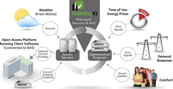
Figure 1 contains a schematic illustration of the BuildingIQ solution. In the image, the term NOC stands for network operations center.

Source: BuildingIQ

(16)

3

Figure 2 shows the data flow process from the onsite BAS to the BuildingIQ appliance with “Site Agent” software and to the BuildingIQ Cloud. The BuildingIQ site agent is software that is installed on site on an appliance which can be supplied by BuildingIQ or by the site.

Figure 2: BuildingIQ data flow

Figure 3 shows how the PEO algorithm aims to exercise temperature control between upper and lower control limits.

Source: BuildingIQ

Figure 3: Optimized temperature control between upper and lower control limits

2.2 Demonstration Sites

2.2.1 Site Selection Criteria

To select suitable sites for the BuildingIQ demonstration, initial meetings were held with the BuildingIQ team to identify a portfolio of ideal demonstration sites to conduct a suitable technology validation. Site selection criteria were developed based on the performance objectives summarized in Table 1. Detailed site selection criteria are provided in Appendix A. Desired site characteristics include:

● Minimum floor area > approximately 100,000 square feet (ft2₎

(17)

4

● Mechanical systems with a central plant and AHUs or large package rooftop units (RTUs) with variable-frequency drives (VFDs) and modulating chilled water valves/multiple compressors

● VAV system

● Direct digital control (DDC) at least to the level of the AHUs ● Whole-building-level metering

● A building- or regional-level point of contact with the willingness and knowledge to provide evaluation information

In addition to these criteria, there are requirements of the site that are necessary to support the installation, configuration, and tuning of the PEO technology. These are detailed in Section 4.6 Scale Up Considerations.

2.2.2 Site Descriptions

The five sites at which the PEO was installed for evaluation are summarized in Table 2. PEO provided optimized setpoints for space air temperature in GSA Chamblee IRS Annex site and for AHU/RTU supply air temperature and duct static pressure in the other four sites. Detailed site characteristics are provided in Appendix B.

Table 2: Cohort of demonstration sites

Site Location Size (ft2₎ _{HVAC System*} _{Control Baseline in Occupied Hours**}

California State University (CSU) Chancellor’s Office Long Beach, CA

168,000 A central chiller/boiler plant as well as 1 AHU equipped with variable frequency drive (VFD) supply fans

AHU supply air temperature setpoint is reset based on outdoor air

temperature. AHU duct static pressure setpoint is a fixed value.

General Services Administration (GSA) Dayton Courthouse Dayton, OH

168,140 A central chiller/boiler plant as well as 7 AHUs equipped with VFD supply fans

Both AHU supply air temperature and duct static pressure setpoints are reset based on VAVterminal damper positions. New York- Presbyterian (NYP) Allen Hospital New York, NY

300,000 15 rooftop units (RTUs) equipped with VFD supply fans

RTU supply air temperature setpoint is reset based on return air temperature. RTU duct static pressure setpoint is a fixed value.

District of Columbia Woodson High School

Wash., DC 235,000 A central chiller/boiler plant, as well as 7 AHUs and 10 RTUs equipped with VFD supply fans

Some of the AHU and RTU supply air temperature setpoints are reset based on return air temperature and the rest are fixed values. The duct static pressure setpoints are fixed values. GSA Chamblee

IRS Annex

Chamblee , GA

387,627 A central chiller/boiler plant as well as 27 AHU equipped with VFD supply fans (serve 280 VAV/PIU terminal units)

Space air temperature setpoints are fixed values.

* Except for the high school, all sites featured reheat at the VAV terminal boxes

** The HVAC system in all sites operates in occupied and unoccupied modes. During unoccupied hours, the system is off.

(18)

5

This cohort reflects climatic diversity, spanning the Southern California (ASHRAE Zone 3B dry), Midwest (ASHRAE Zone 5A cool humid), Northeast and Mid-Atlantic (ASHRAE Zone 4A mixed humid), and Southeast (ASHRAE Zone 3A warm humid) regions. It also represents diversity in commercial building types, including offices, as well as an educational and a healthcare facility. These are near-term key target verticals for BuildingIQ within the commercial sector.

3. Verification and Validation Methodology

This section details the methodology that was used to validate the performance of the PEO technology at each of the five demonstration sites. It covers energy and utility cost savings, as well as impacts to occupant comfort and overarching considerations for technology scale-up.

3.1 Energy and Utility Cost Savings

3.1.1 Savings Estimation Approach and Data Sources

The standard PEO offering includes a proprietary measurement and verification (M&V) module to estimate HVAC energy savings. However, the M&V of energy and utility cost savings reported in this document did not rely on the calculations in that M&V module. Instead, the evaluation team conducted an independent assessment of energy and utility cost savings compliant with the International Performance Measurement and Verification Protocol (IPMVP) (EVO 2012), using Option B and Option C. Option B quantifies HVAC system energy savings through isolated measures of system load, while Option C quantifies savings at the whole-building level. The whole-building energy savings calculations (Option C) were used to as a validity check for the Option B assessments. The research team leveraged the metering, trending, data integration, and storage capabilities that are included in the PEO technology (and associated BAS), and installed additional meters where necessary. Figure 4 shows a snapshot of the BuildingIQ portal with data streams available for viewing and download.

(19)

6

Figure 4: PEO dashboard showing trends of meter and BAS trend log data

Table 3 summarizes the meter data that was acquired at each site to verify energy and utility cost savings. Appendix C contains the electrical metering specifications and submetered locations for each site.

Table 3: Data collected at each site to determine energy and utility cost savings

Quantity Measurement Level of Measurement

Source Whole-building electricity 15-minute interval

kilowatt (kW) data

Whole building On-site meter HVAC electricity 15-minute interval

kW data

Submeters to isolate HVAC loads

On-site meter Whole-building gas 15-minute interval

energy or demand data

Whole building On-site meter

Local outside air temperature Hourly data Area-local Weather Underground data feed

Site-specific utility tariff proxies

n/a n/a BuildingIQ- and

site-provided information Other factors (i.e., building

usage, occupancy levels, space changes, upgrade implementations)

n/a n/a Regular discussion with site operations staff

(20)

7

Under IPMVP Options B and C, energy savings are estimated as defined in Equation 1. A mathematical baseline model is created from data when the technology is not operating. This model characterizes energy use based on key drivers such as time and weather conditions. The baseline model is then forward projected into the measure post-installation verification period to determine what the energy use would have been in the absence of the technology. The difference between this baseline projected energy use, and the metered post-installation energy use is taken as the energy savings. The Adjustments term is used to capture the effects of variables not included in the baseline model and not associated with the technology, such as increased internal loads, or changes to equipment or building occupancy. In addition to the IPMVP, the principles of ASHRAE Guideline 14 (ASHRAE 2014) were applied wherever possible, to inform the evaluation of site energy and cost savings. The guideline provides both quantitative and qualitative recommendations for the baseline period, construction of the baseline model, and the quantification of savings.

Savings = Baseline Energy-Post Installation Energy ± Adjustments (1)

In the application of the Option B approach, the HVAC load was isolated using submeters to capture the HVAC electricity use, and whole-building measures of gas (in the buildings where gas data were available, the majority of building gas consumption was attributed to space conditioning). In the application of the Option C approach, the whole-building energy use was taken as the sum of the whole-building electricity and whole-building gas (where available). Equations 2-5 define the whole-building baseline and post-installation energy and also the HVAC baseline and post-installation energy use.

Whole building Baseline Energy = BElect + BNG (2)

Whole building Post-Installation Energy = PElect + PNG (3)

HVAC Baseline Energy = HVACElect + BNG (4)

HVAC Post-Installation Energy = PHVACElect + PNG (5)

Where

BElect = whole-building baseline electricity BNG = whole-building baseline gas

P Elec = whole-building post-installation electricity PNG = whole-building post-installation natural gas HVACElect = HVAC baseline electricity

PHVACElect = HVAC post-installation electricity

Three statistical goodness of fit metrics were used to verify the accuracy of the baseline models that were created: the coefficient of determination (R2_{), the normalized mean bias error (NMBE),}

and the coefficient of variation of the root mean squared error (CV(RMSE)). These metrics are used to characterize different aspects of model error. Formulas to compute these metrics can be

(21)

8

found in common statistical references, and are provided in Appendix D; CV(RMSE) and NMBE are described in ASHRAE Guideline 14 (ASHRAE 2014).

Utility cost savings were estimated based on achieved energy savings, and either a blended site-specific average utility rate based on historic utility bills, or where applicable, more granular estimates of time-of use costs. Since actual utility costs are assessed at the whole-building level while the field validation assessed HVAC-level savings (versus a 10 percent target), the utility cost savings that were calculated are not equivalent to site-level reductions in actual utility bills over the evaluation period.

3.1.2 Form of the Baseline Model and Definition of the Baseline and Post Installation Period The baseline model that was used to characterize building energy use is a piecewise linear regression that relates load to time-of-week and outside air temperature. Hourly weather data were collected from the sites where the technology was installed and used in the model. This model is defined in detail in the literature, and has been tested and shown to predict energy use with a high degree of accuracy (Granderson et al. 2015; Granderson et al. 2016; Mathieu et al. 2011). The predicted energy consumption is a sum of two terms: (1) a “time of week effect” that allows each time of the week to have a different predicted energy consumption from the others, and (2) a piecewise-continuous effect of temperature. The temperature effect is estimated separately for periods of the day with high and low energy consumption, to capture different temperature slopes for occupied and unoccupied building modes.

Once the site agent was installed and configured at a site, the BuildingIQ system was placed in a 30-day “learning mode” period followed by a 45-day “tuning mode” period. After the tuning period was completed, the HVAC system operations were automatically toggled weekly between standard operations (PEO off) and optimized operations (PEO on). Data from the weeks in which the PEO did not run (PEO off) weretaken as baseline data, while data from the weeks in which the PEO did run (PEO on) were taken as post-installation data. This approach is consistent with that outlined in IPMVP 2012, Section 4.5.2 on Measurement Period Selection (EVO 2012).

3.2 Occupant Comfort Impacts

To verify that the HVAC energy savings gained from PEO were not achieved at the expense of occupant comfort, three types of analysis were conducted.

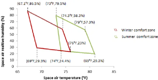
1. Changes in space conditions relative to the ASHRAE thermal comfort zone:This analysis used a simplified model of the ASHRAE thermal comfort zone (ASHRAE 2013), shown in Figure 5. In this model, regions of comfort for winter and summer are defined by boundaries on a plot of relative humidity versus air temperature, as measured in the interior space. To analyze the impact of the PEO on comfort conditions, the fraction of points outside of the comfort zone when the PEO is on is compared to that when the PEO is off. This indicates whether the PEO-governed controls resulted in a change into, or out of, the ASHRAE thermal comfort zone. The space air temperature was acquired from the BAS trend logs for the VAV terminal units. Since measurements of relative

(22)

9

humidity were not available at the zone level, the relative humidity of the space air was estimated in a two-step calculation, also drawing from the BAS trend log data. First, the AHU/RTU return air temperature and relative humidity were used to calculate the specific humidity of the return air. Second, the specific humidity of the return air and the space air were assumed to be approximately equal. The space air relative humidity was then calculated based on the approximated value of the specific humidity. Appendix E contains a detailed description of these calculations.

Figure 5: A simplified representation of the ASHRAE thermal comfort model, with comfort as a function of relative humidity and air temperature

2. Changes in stability of space air temperature: ASHRAE Standard 55 (ASHRAE 2013) specifies the maximum change in operative temperature allowed during specified time periods. The standard states that the operative temperature may not change more than 2°F during a 15-minute period, 3°F during a 30-minute period, 4°F during a one-hour period, 5°F during a two-hour period, or 6°F during a four-two-hour period. To determine the impact of the PEO on space air temperature stability, the number of departures from the maximum specified changes were compared during the time periods when the PEO was on versus when it was off.

3. Changes in hot/cold trouble calls: The evaluation team worked with the site building operations staff to track hot/cold trouble calls. The number of trouble calls from the time periods when the PEO was on was compared to those from the time periods when it was off.

3.3 Technology Scale-Up Considerations

Conclusions regarding technology scale-up and broad-scale applicability were important desired outcomes of the field validation, so factors such as setup and integration effort, tuning and troubleshooting, impact on building management activities, and training, were also included in the evaluation. Bi-weekly calls were held with site operations staff over the duration of the field

(23)

10

assessment. These calls provided information to document staff experiences installing and using PEO. In addition, the evaluation team conducted short, directed interviews with site points of contact after installation and configuration, and at the end of the evaluation. These questions are provided in Appendix F.

Finally, scale-up was evaluated in terms of HVAC system and control requirements, building size and type requirements, and other operational factors that were found to influence savings at each site in the validation cohort. These factors are expected to affect large-scale adoption and deployment of the technology.

4. Demonstration Results

The PEO technology implementation and validation process comprised four main phases: 1. Site agent installation and configuration

2. A 30-day PEO learning mode

3. A 45-day PEO tuning period, to transition control from the BAS sequences to PEO supervisory control

4. A 7–15 month evaluation period during which the PEO was toggled on/off weekly to acquire both baseline data and performance data to verify energy savings and comfort impacts.

The following sections contain validation results from all five sites.

4.1 Baseline ModelingResults

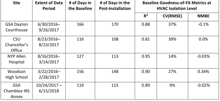
Data were collected throughout the year, capturing varying weather conditions. When the systems were running under standard control (PEO-off mode), the collected data were assigned to the baseline period; when the systems were running under BuildingIQ’s supervisory control (PEO-on mode) the collected data were assigned to the performance, or post-installation period. For each site,1_{the baseline model described in Section 3.1.2 was fit to the data, and the}

goodness-of-fit metrics were calculated. Table 4 summarizes the duration of the data collection period, number of days in the baseline and post periods, and goodness of fit for the baseline models. In three sites, gas data could not be acquired. At Dayton, Chamblee, and CSU the existing gas meters were found to be drastically under-measuring consumption, and at NYP planned installation of a gas meter was never completed, due to factors out of the control of the project team. At the Woodson site, however, whole-building gas data were available, and were included in the baseline model and associated savings analyses.

1_{For one site, CSU, a different baseline model (linear daily) was used to obtain an improved fit over the} time-of-week and temperature model that was suitable for the other sites. The model is described in Appendix G.

(24)

11

Although recommendations vary, “strong” fit is taken as R2_{greater than approximately 0.7,}

CV(RMSE) < 25%, and NMBE < 0.5%. While the values of some of the CV(RMSE) metrics were modestly higher than preferred, overall, the baseline model were deemed sufficient for the savings analysis.

Table 4: Baseline model goodness-of-fit metrics for each site at the HVAC isolation level, for baseline data collected

Site Extent of Data Period

# of Days in the Baseline

# of Days in the Post-Installation

Baseline Goodness-of-Fit Metrics at HVAC Isolation Level

R2 _CV(RMSE) _NMBE GSA Dayton Courthouse 6/30/2016– 9/26/2017 166 170 0.88 37% -0.1% CSU Chancellor’s Office 8/23/2016– 8/23/2017 116 108 0.81 39% 0.0% NYP Allen Hospital 8/16/2016– 3/14/2017 127 113 0.95 14% -0.03% Woodson High School 3/22/2016– 2/28/2017 156 148 0.90 27% 0.34% GSA Chamblee IRS Annex 10/24/2017 – 6/15/2018 119 115 0.89 9% -0.02%

4.2 Energy Savings Results

Table 5 shows the HVAC savings results for each site. In the table, the electricity savings observed at the HVAC submeter levels are presented, followed by the total HVAC savings for the site at which gas data were available. The final column contains the total absolute savings in kilowatt-hours (kWh).

In addition to the tabulated and reported savings determined from the HVAC electricity submeters, the electricity savings indicated at the whole-building meter was used as a cross check. Overall, the savings observed at the HVAC submeter level were consistent with those at the whole-building level; that is, they were in the same range of percent savings observed at the whole-building level, given an assumed fraction of the whole-building load that was attributable to HVAC end uses.

(25)

12

Table 5: HVAC energy savings at each site

Site HVAC Electricity Savings [%] Total HVAC Savings (Electricity + Gas) [%]

HVAC Electricity Savings [kWh] GSA Dayton

Courthouse

1.4 N/A due to poor gas data quality 5,662

GSA Chamblee IRS Annex

CSU Chancellor’s Office

NYP Allen Hospital -0.4 N/A (no gas meter installed) -2,672 Woodson High

School

1.9 1.0 11,425

At CSU, 9 percent HVAC savings were quantified. At the other four sites, savings ranged from 0 to 2 percent. In the following sections each site is further discussed, including an analysis of how savings were achieved, and factors that could have compromised the realization of savings. These analyses were conducted through BAS trend log analysis and interviews with site staff.

4.2.1 CSU Savings Analysis

Nine percent HVAC savings were achieved at the CSU site. Figure 6 shows the average HVAC electricity load for each day of the week. The post-installation condition (PEO on) is plotted in blue, and the baseline projection is shown in red. The difference between the red and blue lines therefore represents the normalized average daily2_{savings throughout the post-installation}

period.

2_{Tuesdays are excluded, as there were insufficient Tuesday data to provide statistically accurate results. This is} because PEO was often switched from on to off, or off to on, on Tuesdays, precluding categorization of the entire 24-hour period as entirely representing either PEO-on of PEO-off operations.

(26)

13

Figure 6: Daily power comparison for the HVAC system time averaged over the 12-month monitoring period at the CSU site

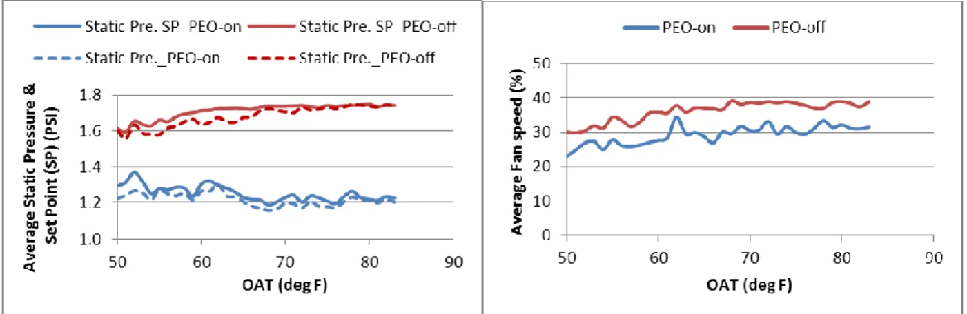
Further analysis showed that this load reduction was in part attributable to a decrease in the AHU static pressure and increase of the AHU supply air temperature affected by the PEO supervisory control. As illustrated in Figure 7, the averaged static pressure in PEO-on mode is 0.4 pounds per square inch (psi) lower than in the PEO-off mode, resulting in a decrease in fan speed. Engineering calculations estimate that the reduction in fan speed caused a 50 percent reduction in fan energy use.

Figure 7: Decrease in AHU static pressure and fan speed at the CSU site (OAT stands for outside air temperature).

In addition to decreases in AHU static pressure, an increase in AHU supply air temperature (SAT) was effected by the PEO algorithm, also contributing to energy savings. Figure 8 shows that when PEO is operating and the outside air temperature is above 60°F the averaged SAT is 0–3 degrees higher than when PEO is not operating (plotted in green). Increasing the SAT has three savings benefits: it reduces cooling energy as it reduces cooling load, it increases the number of hours

(27)

14

when the economizer is able to provide all necessary cooling, and it leads to a decrease in the amount of simultaneous heating and cooling (Murphy 2011).

Figure 8: AHU supply air temperature comparison in PEO-on and PEO-off mode at the CSU site

4.2.2 Savings Analysis for Dayton, Chamblee, NYP Allen, and Woodson

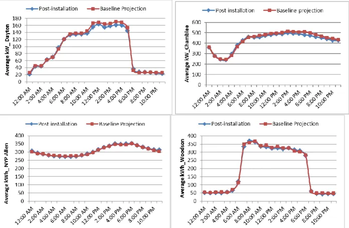
The HVAC savings identified in at the Dayton, Chamblee, NYP Allen Hospital, and Woodson High School sites ranged from 0 to 2 percent. Following the convention used in Figure 6, Figure 9 shows the average HVAC electricity load for each hour of the day at the four sites during the post-installation period. In contrast to the savings clearly visible in Figure 6, these plots show little difference between the post-installation (PEO-on) case and the baseline case (projected to represent what the load under conventional operations would have been during times when PEO was active). A more detailed break out of saving results including monthly and seasonal savings for the Chamblee site is provided in Appendix H.

(28)

15

Figure 9: Time-averaged HVAC power comparison at the Dayton (top left), Chamblee (top right), NYP Allen (bottom left), and Woodson (bottom right) sites; red indicates the baseline projected load for

each hour of the day, and blue indicates the metered load under PEO-on controls.

Complementing the time averaged power plots, Appendix I contains analysis of the AHU static pressure and supply air temperature during PEO-on and PEO-off periods of operation at one of the sites that did not achieve significant savings. The data shown are analogous to that in Figures 7 and 8 for CSU, however in contrast, do not reflect similar energy-saving changes in operational values of these parameters. Further analysis of the issues that may have compromised savings at the three sites (other than CSU) was conducted, and the findings were confirmed through discussion with the operations staff at each site. The issues are summarized below.

GSA Dayton Courthouse

Fixed chilled water (CHW) valve position control requirement: PEO setpoints could not be met in AHU-1, as its CHW valve was continuously locked at the 50 percent or 42 percent open position to maintain minimum flow to the chiller. AHU-1 is the biggest among the seven AHUs and serves approximately 35 percent of the building load.

Baseline reset strategy based on terminal boxes damper positions: In the baseline control case, SAT and static pressure setpoints are reset based the damper positions of all of the terminal units

(29)

16

associated with the AHU. This is an advanced control strategy, as the setpoints are continually adjusted based on actual zone loads. It is possible that the optimal setpoints from the PEO algorithm were equally (but not more) effective as those in the baseline strategy.

GSA Chamblee IRS Annex

Aggressive reset strategies already deployed in the baseline control system: The optimal ZAT setpoints are dynamically determined within a pre-defined minimum and maximum range, and then automatically implemented across 280 perimeter and interior zone VAV terminal units over six floors. However, in the baseline control case, the ZAT already followed heating and cooling setpoints. Table 6 shows the comparison of the ZAT setpoint range during the occupied hours for the baseline and PEO optimal control scenarios. In the perimeter zones, both heating and cooling are provided. The ZAT is controlled between 71°F and 76 °F in the baseline control case, and between 70 °F and 77 °F in the optimal control case. In the interior zones, only cooling is provided. The ZAT is controlled at 73 °F or 74 °F in the baseline control case and at a value between 74 °F and 76 °F in the optimal control case. The comparison suggests the ZAT optimal control setpoints are at most 1 to 2 °F over the baseline, therefore affording very limited savings potential.

Table 6: Comparison of zone air temperature (ZAT) setpoint range in perimeter and interior zones under baseline and PEO-optimized control cases at GSA Chamblee IRS Annex

Control Scenario Perimeter Zone Interior Zone Baseline control of ZAT setpoint range _{71-76 °F} _{73 or 74 °F} PEO optimal control of ZAT setpoint range 70-77 °F 74-76 °F NYP Allen Hospital

Partial capacity of RTUs: Just prior to the installation of the PEO system, new RTUs were installed at the NYP Allen Hospital. However, these new RTUs were not running to full capacity. Half of the RTUs were at 50 to 60 percent of the capacity due to the refrigerant undercharge or issues with the compressor, constraining the extent to which the systems could be exercised for optimization.

Humidity and pressure control requirements: The hospital had strict humidity control requirements in non-operation rooms and pressure control requirements in clean supply rooms. The AHU was set to automatically dehumidify the supply air when return air humidity was greater than 65 percent. This resulted in the SAT overshooting the PEO SAT setpoint. In addition, the VAV boxes served both the patient rooms and clean supply rooms. If the PEO reset the RTU duct static pressure setpoint too low, the space pressure requirements in the clean supply room were not met. The PEO setpoints were frequently overridden due to compensatory adjustments made by the operators to meet zone pressure setpoints.

(30)

17

Incomplete control of full HVAC load: The PEO system was (intentionally) not configured to control the RTUs that served the hospital operation theaters. These RTUs comprised approximately 20 percent of the building cooling load, limiting the portion of total HVAC load under PEO’s control.

Woodson High School

Humidity control requirements: An analysis of the data showed that PEO setpoints could not be met due to required humidity control at the site. The chilled water valve was fully open to maintain space relative humidity at equal to or less than 50 percent, causing the supply air temperature to overshoot the PEO SAT setpoint. This was observed to occur across a set of units that served ~28 percent of the total building cooling load.

Poor controllability of chilled water valve position and supply fan speed: Table 7 summarizes mechanical issues that affected the controllability of chilled water valve position and supply fan speed. These issues were observed in units that served approximately 12 percent of the total building cooling load.

Table 7: Mechanical issues detected at Woodson High School

Unit Issue

AHU 6 Chilled water valve position at 0% all the time after May 3, 2016; Fans operated at 30%/0% during occupied/unoccupied hours before May 3, and 100%/30% during occupied/unoccupied hours after May 3

RTU1 Chilled water valve position at 0% and outside air damper at 100% open all the time; fans operated at 100% at all times

RTU 5 Supply air temperature < outside air temperature and return air temperature when CHW valve was fully closed, possibly due to chilled water valve leakage

RTU 6 CHW valve position at 0% most of time during March to September, 2016

Incomplete control of full HVAC load: The BuildingIQ system was (intentionally) not configured to control two of the dedicated outdoor air system (DOAS) units that served approximately 23 percent of the building load.

Overrides and reheat: For unknown reasons, a third-party contractor intermittently overrode the PEO control. Additionally, reheat is not used at the Woodson site, as the boilers were shut down from April through October. Absence of reheat limits the savings potential, as there is no simultaneous heating and cooling to minimize.

(31)

18

Overrides and reheat: For unknown reasons, a third-party engineer intermittently overrode the PEO control. Additionally, from April through October, the period in which boilers were shut down for the season, VAV reheat was not possible, thus there was less savings potential, as there was no simultaneous heating and cooling to reduce.

4.3 Occupant Comfort Results

As outlined in Section 3.2 thermal comfort impacts were assessed by analyzing changes with respect to the ASHRAE comfort zone, the stability of space temperature, and records of trouble calls. Taken as a whole, the data analyses indicate a relatively modest increase in discomfort conditions when PEO was in active control, in most zone spaces sampled.

4.3.1. Comfort Zone Analysis

The analysis of comfort using the simplified ASHRAE comfort model as described in Section 3.2 was performed at the Dayton, Woodson and Chamblee test sites where the zone temperature measurements in VAV boxes were available. Data were gathered from a set of AHUs and associated VAV boxes representative of standard occupied spaces. For each AHU, two linked VAV boxes that serve regular office or classroom spaces were studied. The targeted AHUs (AHU-3, -4, and -7) were those that serve the third, sixth, and seventh floors of Dayton site, those that serve the third, fourth, and fifth floors of Chamblee site (AHU 3-2, 4-3, and 5-1), and those that serve the first and third floors of Woodson site (AHU-3 and RTU-9). The analysis time period only included the hours when the building was heavily occupied (Dayton and Chamblee, weekdays from 8:00am to 5:00 p.m.; Woodson, weekdays from 8:45 a.m. to 3:15 p.m.) The data collected at Dayton spans January 5, 2017, through June 19, 2017. The data collected at Woodson spans April 1, 2016, through February 23, 2017. The data collected at Chamblee spans November 1, 2017, through May 30, 2018.

The analysis was conducted for 3 AHUs and 6 associated VAV boxes at Dayton, for 2 AHUs and 4 associated VAV boxes at Woodson, and 3 AHUs and 6 associated VAV boxes at Chamblee. Figure 10 shows the results when each of the 16 VAV zones was considered individually. In 2 out of 6 Dayton site zone spaces, the PEO operations showed a slight increase in the number of points outside of the comfort zone. In all 10 of the Woodson and Chamblee zone spaces, the PEO operations showed a modest increase in the number of points outside of the comfort zone.

(32)

19

Figure 10: Percentage of operational points (space temperature paired with space humidity) outside of the comfort zone for each VAV, during the PEO-on (blue) and the PEO-off (red) time periods at

Dayton Courthouse, Woodson High School, and Chamblee IRS Annex

4.3.2 Space Air Temperature Stability

ASHRAE Standard 55 defines the maximum space air temperature changes allowed over several time periods: 15 minutes, half an hour, one hour, two hours, and four hours. Each of the VAV boxes that were analyzed according to the simplified thermal comfort model was also analyzed to evaluate departures from these temperature stability thresholds. Table 8 summarizes the number of times that the space air temperature at the Dayton and Woodson sites changed by an amount greater than that allowed under the ASHRAE standard. Across each of the 10 zone spaces, and each of the time periods, there were 448 instances of departures from the standard when the PEO was not operational and 310 instances when the PEO was operational. These data indicate that the PEO-governed controls may have modestly improved space temperature stability.

Table 8: The number of times that the change in space air temperature exceeded the maximum allowable during the studied time period, for each time duration in ASHRAE Standard 55

PEO Status Dayton - Time Duration (hours)

Woodson - Time Duration (hours)

Chamblee – Time Duration (hours) 0.25 0.5 1 2 4 0.25 0.5 1 2 4 0.25 0.5 1 2 4 Baseline (PEO off) 13 25 25 46 36 5 23 44 122 96 0 3 4 6 0 Performance (PEO on) 7 6 14 21 14 4 17 29 87 96 3 5 5 2 0

(33)

20

The evaluation team worked with the site points of contact to track trouble calls for hot and cold complaints from building occupants during the PEO-on and PEO-off periods. This analysis was conducted for the NYP Allen and CSU sites, where records of trouble calls were maintained and accessible for evaluation.

Table 8 shows that the number of recorded hot and cold calls did not change dramatically at NYP Allen during times of PEO operation, and may have decreased at CSU. Interestingly, when surveyed, the staff at NYP Allen hospital and Dayton suggested that there were more trouble calls when BuildingIQ was in control, and that in response they frequently override the PEO setpoints. It was noted that a portion of the trouble calls at NYP Allen hospital were issued through direct phone calls and not included in the electronic record represented in Table 9.

Table 9: Hot and cold complaints record from sites

Site Dates tracked

Trouble calls

Baseline (PEO-off) Post-installation ( PEO-on) NYP Allen 8/16/2016–3/14/2017 917 805

CSU 9/7/2016–6/30/17 16 5

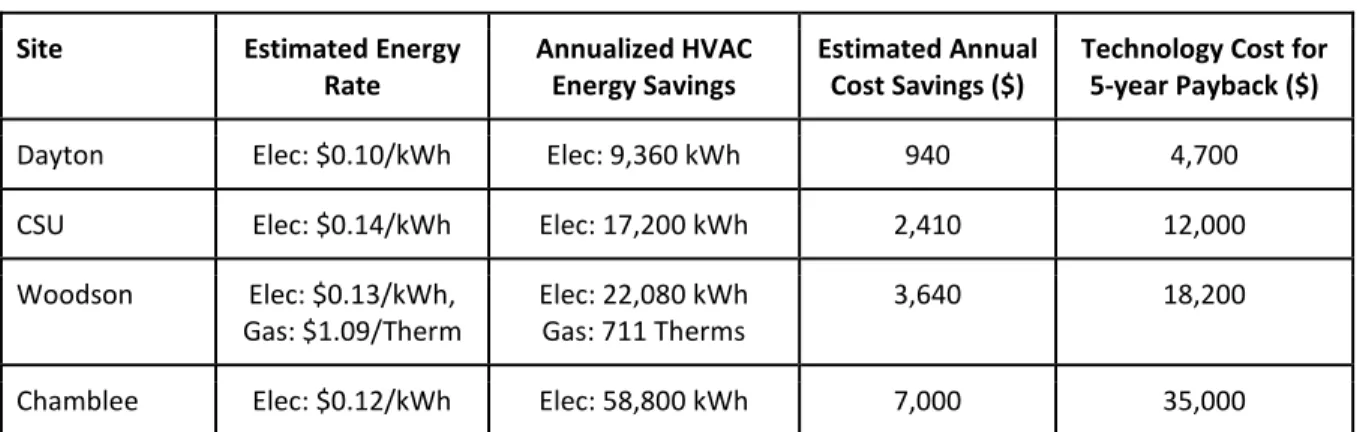
4.4 Cost Savings and Payback Analysis

Cost savings and payback analysis was conducted for the four sites that have positive savings. Table 10 summarizes the estimated utility energy rate, as well as the annualized HVAC energy savings, and estimated annual cost savings. Utility rates were estimated by aggregating utility bills and consumption over a 12-month period to determine a blended average cost of electricity per kilowatt-hour or cost of gas per therm.

Estimated annual cost savings were calculated from the percent (i.e., fractional) HVAC savings, the baseline-predicted 12-month predicted HVAC energy use, and the estimated energy rate, as defined in Equation 9. Fractional savings were calculated according to ASHRAE Guideline 14 guidance, and the 12-month predicted energy use was calculated from the baseline model using measured 12-month outside air temperature data (from Weather Underground).

𝐶𝑜𝑠𝑡 𝑠𝑎𝑣𝑖𝑛𝑔𝑠 = 𝑓𝑟𝑎𝑐𝑡𝑖𝑜𝑛𝑎𝑙 𝑠𝑎𝑣𝑖𝑛𝑔𝑠 ∗ 12𝑚𝑜. 𝑝𝑟𝑒𝑑𝑖𝑐𝑡𝑒𝑑 𝑘𝑊ℎ ∗ 𝑒𝑛𝑒𝑟𝑔𝑦 𝑟𝑎𝑡𝑒 (9)

Generalized market costs for the “make ready” installation integration and configuration of PEO or ongoing annual software and services fees were not available to the evaluation team in this validation study. This was because the study was supported through a competitively awarded process that included cost share contributions from each site as well as from BuildingIQ, and these contributions were applied to cover the cost of the technology. Therefore, rather than an

(34)

21

achieved payback analysis, the required total five-year technology cost to meet a simple five-year payback was calculated and shown in Table 10.

Table 10: Estimated cost savings and technology costs to meet a five-year payback

Site Estimated Energy Rate

Annualized HVAC Energy Savings

Estimated Annual Cost Savings ($)

Technology Cost for 5-year Payback ($) Dayton Elec: $0.10/kWh Elec: 9,360 kWh 940 4,700 CSU Elec: $0.14/kWh Elec: 17,200 kWh 2,410 12,000 Woodson Elec: $0.13/kWh,

Gas: $1.09/Therm

Elec: 22,080 kWh Gas: 711 Therms

3,640 18,200

Chamblee Elec: $0.12/kWh Elec: 58,800 kWh 7,000 35,000

A BuildingIQ field evaluation conducted by San Diego Gas & Electric (SDG&E 2015) yielded savings of 10.7 percent, and was able to capture complete costs, reporting a payback of 6.5 years.

4.5 Ongoing Commissioning

In addition to the implementation of the PEO control strategies, BuildingIQ conducted ongoing building commissioning-type activities throughout the evaluation period. BuildingIQ highlighted issues which could impact performance overall, as well as the effectiveness of PEO. Several of the key findings by BuildingIQ that impact building performance are described below.

BuildingIQ confirmed for one of the sites that the daily start-up time of each AHU was significantly earlier than necessary. Early start-up extends the hours that the building is in operation, thereby expending more energy. By adjusting the start-up time, additional energy savings could be realized.

At another site, BuildingIQ identified a boiler control panel problem and that problem was fixed during the project. The fixed boiler control panel would lead to significant gas savings, as the boiler hot water supply temperature setpoint can be reset according the programed control sequence rather than remain at a fixed high value.

BuildingIQ frequently noted overridden control points, such as fan speed, supply air temperature setpoint, chilled water valve position, and hot water valve position. These overrides had the effect of locking a unit into a specific state, which could lead to wasted energy or to challenges meeting thermal comfort conditions. Additionally, overrides to supply air temperature setpoint, fan speed, and duct static pressure setpoint could constrain PEO from implementing optimal strategies, thus limiting potential energy savings. BuildingIQ frequently alerted sites of such overrides, the release of which would contribute to significant energy savings.

(35)

22

BuildingIQ also noted issues where system capacity appeared to have been reached. In these cases, the unit appeared to be operating correctly, with a fan running at 100 percent speed, or a water coil valve open to 100 percent for extended periods of time. It is possible that during these times thermal comfort conditions were not satisfied.

BuildingIQ highlighted numerous issues with AHUs in addition to overridden values and capacity limits noted earlier. They called out instances where an AHU fan ran at 100 percent throughout the entire occupied period; outside air dampers were noted for excessive cycling and being fully open during unfavorable outside air conditions; chilled water and hot water valves were documented for excessive cycling (probably due to loop tuning issues) and being physically stuck or locked at a particular position. BuildingIQ also noted instances where zone temperature sensors appeared to have failed.

4.6 Scale-up Considerations

Scale-up considerations extend beyond energy and cost savings into issues related to ease of technology adoption, and general usability. The findings reported in the following subsections comprise information obtained from interviews with key points of contact at each demonstration site, as well as observations from the evaluation team.

4.6.1 Implementation Lead Time

The standard process to implement the PEO solution consists of a period of installation and configuration (including system integration), followed by an approximately 30-day “learning mode” period and an approximately 45-day “tuning” period. During the learning period, the PEO algorithms and models are fit to the specific site, using measured operational and energy use data. During the “tuning period,” the optimized control is gradually brought on as the building is transitioned from conventional control to fully into the control of the PEO. Figure 11 shows BuildingIQ implementation lead times for the four locations studied.

(36)

23

Across the validation sites, the duration of the installation and configuration phase generally ranged from 7 to 12 weeks. At one site, over six months was required due to extended delays in IT approvals. At another site, eight months was required to obtain approval to perform zone-level control and to map and configure BAS data points at the AHU and zone levels. The duration of the learning and tuning phases was not indicative of typical PEO deployments, as they were significantly extended (by many months) due to project-specific circumstances. Specifically, additional time was required to install submetering equipment and collect baseline data for performance verification; additionally, and at two sites the BAS servers were upgraded or reconfigured as part of general maintenance activities that were independent of the BuildingIQ installation.

4.6.2 Staff Engagement

The most common activities that were required of the on-site engineer or primary organization point of contact during the installation and system integration phase are summarized below:

● Interfacing between the BAS controls contractor and the BuildingIQ team

● Interfacing with the IT department to acquire approvals and permissions for technology installation

● Provision of control specifications and sequences to the BuildingIQ team ● Provision of device and system access to the BuildingIQ team

● Scheduling site access and site walkthroughs ● Testing software configurations and connectivity

● Monitoring space air temperature and humidity, and equipment operation, for stability ● Providing the BuildingIQ team feedback on setpoint changes based on occupant response In general, across four sites, the primary point of contact estimated that 0.5 to 2 weeks of total (non-contiguous) staff time was dedicated to system installation, not including the efforts of IT staff and contractors. In the most difficult case, significantly more staff time was required. In the simplest case, the site had already completed a project to upgrade the BAS for BACnet compatibility, set up of trend logging, and communications connectivity.

For two of four sites, the staff considered the PEO installation and integration process to be more involved than the installation and integration of a traditional BAS. Although PEO provides different functionality than a BAS and is not intended to replace it, BAS are a familiar control technology and therefore provide a useful reference point. This was due largely to IT requirements and the total calendar time required to complete the installation an integration. For the third site—the one that had just completed a BACnet and controls connectivity upgrade— the process required very little additional effort. The fourth site reported that the majority of work was conducted between the BAS contractor and BuildingIQ team, and the fifth site reported that the effort to install and integrate PEO was approximately equivalent that that for a typical BAS.