Vol. 4, No. 2, 2012, pp. [128–147] www.cscanada.net DOI: 10.3968/j.pam.1925252820120402.S0803 www.cscanada.org
Robust Inference for Incomplete Binary
Longitudinal Data
Sanjoy K. Sinha
[a],*[a] School of Mathematics and Statistics, Carleton University, Canada.
* Corresponding author.
Address: School of Mathematics and Statistics, Carleton University, Ottawa, ON, K1S 5B6, Canada; E-Mail: [email protected]
Supported bya grant from the Natural Sciences and Engineering Research Council of Canada.
Received: August 20, 2012/ Accepted: October 10, 2012/ Published: October 31, 2012
Abstract:
Missing data occur in many longitudinal studies. When ta are nonignorably missing, it is necessary to incorporate the missing da-ta mechanism into the observed dada-ta likelihood function. A full likelihood analysis of nonignorable missing data is complicated algebraically, and often requires intensive computation, especially when there are many follow-up times. To avoid such computational difficulties, pseudo-likelihood methods have been proposed in the literature under minimal parametric assumptions. However, like the classical maximum likelihood estimators, these pseudo-likelihood estimators are also sensitive to potential outliers in the data. In this article, we propose and explore a robust method in the framework of a pseudo-likelihood function that is derived under the working assumption that the longitudinal responses are independent over time. The performance of the proposed robust method is investigated in simulations. The method is also illustrated in an example using actual data on CD4 counts from clinical trials of HIV-infected patients.Key words:
Incomplete data; Longitudinal study; Marginal models; Non-ignorable missingness; Outliers; Robust estimationSinha, S.K. (2012). Robust Inference for Incomplete Binary Longitudinal Data. Progress in Applied Mathematics, 4(2), 128–147. Available from http://www.cscanada.net/index. php/pam/article/view/j.pam.1925252820120402.S0803 DOI: 10.3968/j.pam.19252528201 20402.S0803
1. INTRODUCTION
In many longitudinal studies, individuals are measured repeatedly over a fixed set of assessment times. For example, longitudinal data are often collected in AIDS, cancer, and cardiovascular clinical trials as well as in observational studies. Here we focus on the case where the response over time is binary, and we are interested in modeling the marginal means of the binary responses. Methods for analyzing binary longitudinal data have been extensively studied in the literature (e.g., Le Cessie & Van Houwelingen, 1994; Liang & Zeger, 1986; Meester & MacKay, 1994; Molenberghs & Lesaffre, 1994; Prentice, 1988; and many others). In the absence of a suitable likelihood function to work with, often longitudinal data are analyzed using a multivariate analogue of the quasi-likelihood function (Wedderburn, 1974). The development of the “quasi-score equations”, however, requires correct specification of the correlation matrix of the repeated responses over time. Liang and Zeger (1986) suggested a simplified “working” correlation matrix, and argued that the estimators obtained by solving their proposed “generalized estimating equations” (GEEs) are consistent even under a misspecified correlation structure.
The modeling of binary longitudinal data is often complicated by the fact that the response variable is not always observed at all assessment times. If missingness does not depend on the values of the data, missing or observed, then the data are called missing completely at random (MCAR). Any method that yields valid inferences in the absence of missing data would also yield valid inferences when data are missing completely at random and the analysis is based on the available data. A less restrictive assumption than MCAR is that missingness depends only on the observed values of the variables, but not on the values that are missing. In this case, data are called missing at random (MAR). Many authors considered extensions of the aforementioned quasi-likelihood approaches to the analysis of incomplete longitudinal data under the MAR assumption. Robins et al. (1995) proposed a weighted generalized estimating equation (WGEE) approach based on “inverse probability weights” (IPW) for analyzing longitudinal data under the assumption of MAR.
Note that missingness in the longitudinal data often depends on the unobserved value of the response variable at that time. In such cases, the missing data mechanis-m is called nonignorable (Little &amechanis-mp; Rubin, 2002). As an examechanis-mple, here we consider a data set from two clinical trials of HIV-infected patients, initially analyzed by Gallant et al. (1992) and Kahn et al. (1992). In this experiment, 431 patients were diagnosed with AIDS or AIDS-related complex, and the study was designed to compare two therapeutic treatments, zidovudine (Azt) and didanosine (Ddi). The response is a binary CD4 cell count variable, measured at baseline (week 0), and every week for up to 5 weeks from baseline. The interest is on the effect of treatment on changes in CD4 cell count over time. As in many longitudinal stud-ies, here the analysis is complicated by missing response data over time. Although measurements on CD4 cell counts were taken from all 431 patients at baseline, but incomplete measurements were taken from only 383 patients (88.95%) at week 1, 345 patients (80.0%) at week 2, 324 patients (75.2%) at week 3, 306 patients (71.0%) at week 4, and only 285 patients (66.1%) at week 5. The missing data pattern is also non-monotone, that is, some patients’ responses are missing at one visit, but observed at the next visit. There are 109 (25.3%) patients who missed at least one visit, but returned for a later visit. A decline in CD4 count normally
indicates disease progression, and patients with low CD4 counts are more likely to make all scheduled visits, as compared to patients with normal CD4 counts. This would imply that missingness in the CD4 cell counts depends on the unobserved outcome and so is “nonignorable”.
Statistical analyses with missing data based on the likelihood approach were considered by many authors (e.g., Brown, 1990; Dantanet al., 2008; Diggle & Ken-ward, 1994; Ibrahim et al., 1999, 2001; and Sinhaet al., 2010, 2011). Ibrahim et al. (1999) propose an EM algorithm for maximum likelihood estimation in gener-alized linear models for data with nonignorable missing covariates. Ibrahim et al. (2001) extended the EM method to the analysis of generalized linear mixed models with nonignorable missing responses. Recently, Sinha et al. (2010) investigates a multivariate logistic regression model for analyzing multiple binary outcomes with incomplete covariate data where auxiliary information is available. The auxiliary data are extraneous to the regression model of interest but predictive of the covariate with missing data.
A full likelihood analysis of longitudinal data under nonignorable missingness of-ten requires inof-tensive computation, especially when there are many follow-up times. To overcome this problem, a pseudo-likelihood approach was proposed by Troxelet al. (1998) under minimal parametric assumptions. This pseudo-likelihood approach was developed under the working assumption that the longitudinal outcomes are independent over time, and yields asymptotically unbiased estimators of the regres-sion parameters when the marginal model for the response at each time-point and the model for missingness have been correctly specified.
It is well-known that the ordinary maximum likelihood and maximum pseudo-likelihood estimators are sensitive to potential outliers in the data. To bound the influence of outliers, robust methods were studied by a number of authors (e.g., Can-toni & Ronchetti, 2001; Preisser & Qaqish, 1999; Sinha, 2004). Most of these robust methods focused on the estimation in generalized linear models in a complete-data setting. Sinha (2004) proposed a robust method for analyzing clustered correlated data in the framework of maximum likelihood approach for generalized linear mixed models. Also, Sinha (2008) proposed a robust method for fitting generalized linear models with nonignorable missing covariates.
In this paper, we focus on a robust analysis of longitudinal binary data with nonignorable missing responses. As mentioned earlier, a full likelihood analysis of nonignorable missing data typically involves intensive computation. Here our goal is to adopt a suitable method which is computationally feasible and also provides robust estimators in the presence of potential outliers in the data. In this note, we consider a robust method in the framework of the pseudo-likelihood of Troxel et al. (1998). The proposed method requires much less computation as compared to the full likelihood analysis of binary longitudinal data. Note that in the case of binary data, although no outliers are desired in the binary outcomes, outliers are still important in the residual sense; standardized residuals could be unbounded for a binary model. The proposed robust method is useful for bounding the influence of both outliers in the residuals and leverage points in the design space.
The paper is organized as follows. Section 2 introduces the model and notation for analyzing longitudinal data. Section 3 introduces the proposed robust method and studies the asymptotic properties of the robust estimators. Section 4 provides an illustrative example to describe the computational issues of the robust estimation. Section 5 investigates the empirical properties of the robust estimators based on a
simulation study. Section 6 presents an application of the proposed method using the CD4 cell count data introduced earlier. Section 7 concludes the paper with some discussion.
2. MODEL AND NOTATION
SupposeN individuals, i= 1, . . . , N, are observed at a fixed set ofT time-points,
t= 1, . . . , T. Letyi represent a T×1 vector of repeated responses, (yi1, . . . , yiT),
for theith individual. Also, letxit represent ap×1 vector of covariates associated
with the response yit for individuali at timet. We assume that all the covariates
are fully observed.
The marginal distribution ofyitis assumed to be Bernoulli with the probability
of success pit=E(yit|xit,β) =P(yit= 1|xit,β) = exp(xtitβ) 1 + exp(xt itβ) . (1)
Here our goal is to draw inferences about the regression parametersβ, whereas the within-subject association among the repeated outcomes is regarded as a nui-sance characteristic of the data. The association between a pair of binary outcomes is typically measured in terms of marginal correlations or marginal odds ratios. Marginal correlations can be used to derive a multivariate Bahadur (1961) model, whereas marginal odds ratios can be used to derive a multivariate Plackett (1965) distribution.
We focus on the case where individuals in a longitudinal study are not observed at all T follow-up times on account of some stochastic missing data mechanism. We introduceT binary random variables, vit,(t= 1, . . . , T), with vit equal to 1 if
the responseyit is observed, and 0 ifyit is missing. We assume that the marginal
distribution of the binary random variablevitis Bernoulli, with the probability of
being observed, πit=P(vit= 1|xit, yit,τ) = exp(τ0+τt1xit+τ2yit) 1 + exp(τ0+τt 1xit+τ2yit) . (2)
Note that ifτ26= 0, then the missing data mechanism is nonignorable since the
probability of missingness depends on possibly unobserved data yit. In the next
section, we briefly review the pseudo-likelihood approach of Troxelet al. (1998) for analyzing incomplete binary longitudinal data, and then introduce our proposed robust method in the framework of this pseudo-likelihood function.
3. ESTIMATORS
3.1. Independent Pseudo-Likelihood (IPL) Estimator
Troxel et al. (1998) proposed a pseudo-likelihood under the working assump-tion that the repeated responses are independent over time. To describe this, let
fy,v(yit, vit|xit,β,τ) be the marginal distribution of (yit, vit) at time t, which can
be expressed as
where fy(yit|xit,β) is Bernoulli with probability of successpit as given in (1), and
fv(vit|xit, yit,τ) is Bernoulli with probability of being observed as given in (2).
Then treating the repeated observations at different follow-up times as independent, Troxelet al. (1998) defined the pseudo-likelihood ofθ= (βt,τt)tby
L(θ) = N Y i=1 T Y t=1 {fy(yit|xit,β)fv(vit|xit, yit,τ)} vit ( 1 X yit=0 fy(yit|xit,β)fv(vit|xit, yit,τ) )1−vit (4) The logarithm of the pseudo-likelihood function may be obtained as
logL(θ) = N X i=1 T X t=1
vit{logfy(yit|xit,β) + logfv(vit|xit, yit,τ)}
+ N X i=1 T X t=1 (1−vit) log ( 1 X yit=0 fy(yit|xit,β)fv(vit|xit, yit,τ) ) . (5)
An estimator ofθmay be obtained by maximizing the pseudo-likelihood function (4) or the log-pseudo-likelihood function (5).
From (5), the pseudo-score equations for the regression parametersβ take the form 0=∂logL(θ) ∂β ≡Sβ(θ)≡ N X i=1 Si,β(θ) = N X i=1 T X t=1 vit ∂logfy(yit|xit,β) ∂β + N X i=1 T X t=1 (1−vit)Ey|v ∂logf y(yit|xit,β) ∂β vit = N X i=1 T X t=1 vit(yit−pit)xit+ N X i=1 T X t=1 (1−vit)Ey|v{(yit−pit)xit|vit}, (6) where Ey|v represents the expectation with respect to the conditional distribution
of the responseyitgiven the value of the missing data indicatorvit.
Similarly, the pseudo-score equations for the parametersτ of the missing data model (2) may be obtained as
0=∂logL(θ) ∂τ ≡Sτ(θ)≡ N X i=1 Si,τ(θ) = N X i=1 T X t=1 vit ∂logfv|y(vit|xit, yit,τ) ∂τ + N X i=1 T X t=1 (1−vit)Ey|v ∂logf v|y(vit|xit, yit,τ) ∂τ vit = N X i=1 T X t=1 vit(vit−πit)zit+ N X i=1 T X t=1 (1−vit)Ey|v{(vit−πit)zit|vit}, (7)
where zit= (xtit, yit)t.
Equations (6) and (7) are solved simultaneously for the “independent pseudo-likelihood” (IPL) estimators ˜θ= ( ˜βt,τ˜t)tof the model parametersθ= (βt
,τt)t.
3.1.1. Standard Errors of IPL Estimators
We can write the pseudo-score functions forβandτ in matrix form as
∂ ∂θS(θ)≡ ∂ ∂θ Sβ(θ)t, Sτ(θ)t t = ∂Sβ(θ) ∂β ∂Sτ(θ) ∂β ∂Sβ(θ) ∂τ ∂Sτ(θ) ∂τ , where ∂Sβ(θ) ∂β =− N X i=1 T X t=1 pit(1−pit)xitxtit + N X i=1 T X t=1 (1−vit) Ey|v{(yit−pit)2|vit} − {Ey|v[(yit−pit)|vit]}2 xitxtit, (8) ∂Sτ(θ) ∂τ =− N X i=1 T X t=1 πit(1−πit)zitztit + N X i=1 T X t=1 (1−vit)Ey|v{(vit−πit)2zitztit|vit} − N X i=1 T X t=1
(1−vit)Ey|v{(vit−πit)zit|vit}Ey|v{(vit−πit)zit|vit}t,
(9) and ∂Sβ(θ) ∂τ = ∂Sτ(θ) ∂βt = N X i=1 T X t=1 (1−vit)Ey|v{(yit−pit)(vit−πit)xitztit|vit} − N X i=1 T X t=1 (1−vit)Ey|v{(yit−pit)xit|vit}Ey|v{(vit−πit)zit|vit}t. (10)
To estimate the asymptotic variance-covariance matrix of the IPL estimators, we can use a sandwich-type variance-covariance matrix in the form
Var(˜θ)≈ ∂S(θ) ∂θ −1(N X i=1 Si(θ)Sit(θ) ) ∂S(θ) ∂θ −1 , (11) where Si(θ) = Si,β(θ)t, Si,τ(θ)t t .
An estimate of the variance of ˜θ is obtained by evaluating the right-hand side of (11) at the IPL estimate ˜θ.
3.2. Proposed Robust Pseudo-Likelihood (RPL) Estimator
Note that in the case of binary longitudinal data, as the responseyis binary, outliers can arise in the data only through the covariates x. We focus on the case where the covariates are continuous, but the method can be generalized for discrete or a mixture of discrete and continuous measurements.
From (6) and (7), it is clear that the pseudo-score functions for β and τ are proportional to the covariatesx, so the influence of an outlier on the ordinary IPL estimators is unbounded. In other words, the IPL estimators are not robust against outliers. To obtain robust estimators of the model parametersβandτ, we propose to solve the estimating equations
N X i=1 Ψβ,i(yi,vi|β,τ) = 0, (12) N X i=1 Ψτ,i(yi,vi|β,τ) = 0, (13) where Ψβ,i(yi,vi|β,τ) = T X t=1 vit{ψc(rit)−Ey{ψc(rit)}}σitwitxit + T X t=1 (1−vit)Ey|v[{ψc(rit)−Ey{ψc(rit)}} |vit]σitwitxit (14) and Ψτ,i(yi,vi|β,τ) = T X t=1 vit ψc(rit∗)−Ev|y{ψc(r∗it)} σit∗wit∗zit + T X t=1 (1−vit)Ey|v ψc(r∗it)−Ev|y{ψc(rit∗)} σ∗itw∗itzit|vit (15)
withrit= (yit−pit)/σit,σit2 = var(yit),rit∗ = (vit−πit)/σit∗, andσ∗
2
it = var(vit). The
functionψc is considered as the Huber’s psi function, ψc(r) = max{−c,min(r, c)},
which is used to bound the influence of any outliers in the residuals when estimating the model parameters.
The weightswit=w(xit) andw∗it=w(zit) are used to downweight any leverage
points in the design space. Here we choose the weight functionw as a function of the Mahalanobis distancedxin the form
w(x) =w(x,cx,Sx) = min ( 1, b 0 dx γ0/2) (16) wheredx= (x−cx)TSx−1(x−cx), the tuning constantsγ0≥1 andb0 is chosen as
the 95th percentile of the chi-squared distribution with degrees of freedom equal to the dimension ofx, and cxand Sx are some robust estimators of the location and
scale parameters for the distribution of x, such as the minimum volume ellipsoid (MVE) estimators of Rousseeuw and van Zomeren (1990). Note that the choice
ψc(r) =r and w(x) = 1 leads to the ordinary pseudo-likelihood (IPL) estimators
3.2.1. Newton-Raphson Method for RPL Estimators
The proposed RPL estimators of β andτ are obtained by solving the estimating equations (12) and (13) simultaneously using an iterative method. We focus on the iterative Newton-Raphson method and the scoring technique for solving these equations. The iterative equations for the RPL estimators of β may be expressed in the form β(m+1) = β(m)− (N X i=1 ˙ Ψβ,i(yi,vi|β(m),τ) )−1 N X i=1 Ψβ,i(yi,vi|β(m),τ),(17) form= 0,1,2, . . ., where ˙ Ψβ,i(yi,vi|β,τ) = T X t=1 vit ∂ ∂ηit {ψc(rit)−Ey{ψc(rit)}} σitwitxitxtit + T X t=1 (1−vit)Ey|v ∂ ∂ηit {ψc(rit)−Ey{ψc(rit)}} vit σitwitxitxtit.
Similarly, the iterative equations for the RPL estimators ofτ can be expressed in the form τ(m+1) = τ(m)− (N X i=1 ˙ Ψτ,i(yi,vi|β,τ(m)) )−1 N X i=1 Ψτ,i(yi,vi|β,τ(m)),(18) form= 0,1,2, . . ., where ˙ Ψτ,i(yi,vi|β,τ) = T X t=1 vit ∂ ∂ηit ψc(rit∗)−Ev|y{ψc(r∗it)} σit∗wit∗zitztit + T X t=1 (1−vit)Ey|v ∂ ∂ηit ψc(r∗it)−Ev|y{ψc(rit∗)} σ ∗ itw ∗ itzitztit vit .
The complete algorithm for these robust estimators ofβ and τ is described as follows:
1. Choose initial valuesβ(0) andτ(0). These initial values can be chosen as the ordinary IPL estimates ofβandτ. Setm= 0.
2. (a) Calculateβ(m+1)andτ(m+1)from the iterative equations (17) and (18),
respectively. (b) Setm=m+ 1.
3. Continue step 2 until a convergence is achieved. Declare the estimates at convergence to be the RPL estimates ˆβand ˆτ.
3.2.2. Asymptotics for RPL Estimators
A sketch of the development of the asymptotic distributions of the RPL estimators is given here. Recall the estimating equations (12) and (13) for the robust estimators
ofβ andτ. These equations can be reexpressed in the form GN(y,v|θ) = 1 N N X i=1 Ψi(yi,vi|θ) =0, (19)
where Ψi(yi,vi|θ) = {Ψβ,i(yi,vi|β,τ)t,Ψτ,i(yi,vi|β,τ)t} t . Let ˆθN = ( ˆβ t N,τˆ t N)t
denote the robust estimators obtained by solving (19). Assume that the “true” valuesθ0ofθ are obtained by solving the equations
¯ GN(θ) = 1 N N X i=1 E{Ψi(yi,vi|θ)}=0 (20)
with respect to θ. By the Mean Value Theorem, we can write
GN(y,v|θˆN) =GN(y,v|θ0) +G0N(y,v|θ˜)(ˆθN −θ0), (21)
where vector ˜θ lies on the segment connecting ˆθN and θ0, andG0N(y,v|θ˜) is the
derivative ofGN(y,v|θ) with respect toθevaluated at ˜θ. From (21), we can write √ N(ˆθN−θ0) = n −G0N(y,v|θ˜)o −1n√ NGN(y,v|θ0) o . (22)
Now, the asymptotic normality of ˆθN will follow ifG0N(y,v|˜θ) in (22) converges
appropriately, and if the vector√NGN(y,v|θ0) has the central limit property.
Un-der appropriate regularity conditions as described in Sinha (2004) (see also White, 1982), it can be shown that ˆθN →θ0a.s. andkG0N(y,v|θ˜)−G¯0N(θ0)k→0 a.s. as N → ∞. Also, we can show that√NGN(y,v|θ0) is asymptoticallyN{0,QN(θ0)},
where QN(θ0) = var
n√
NGN(y,v|θ0) o
. Then from (22), we can argue that
√
NQN(θ0)−1/2MN(θ0)(ˆθN −θ0) ˙∼N(0,I), (23)
whereMN(θ) =−G¯N(θ) =−E{G0N(y,v|θ)}. The asymptotic variance-covariance
matrix of the robust estimators ˆθN may be obtained from
VN(θ0) =M−N1(θ0)QN(θ0)M−N1(θ0). (24)
The computational aspects of this variance-covariance matrix are discussed in an illustrative example in the next section.
4. ILLUSTRATIVE EXAMPLE
Here we describe the computational issues of the proposed robust estimator using a simple example. Suppose in a clinical study, yit represents a binary response from
individual iat timet. To describe the success probability pit as a function of time
tand a baseline covariatexi for individuali, consider a marginal logistic regression
model in the form
yit∼Bernoulli(pit), i= 1, . . . , N, t= 1, . . . , T,
Definevit= 1 if the responseyitis observed andvit= 0 ifyitis missing. Assume
that the marginal distribution of the binary random variable vit is Bernoulli, with
the probability of being observed,
πit=P(vit= 1|yit, xi,τ) =
exp(τ0+τ1xi+τ2yit)
1 + exp(τ0+τ1xi+τ2yit)
(26) Here the parameters of interest are the regression coefficientsβ= (β0, β1, β2)t,
with τ = (τ0, τ1, τ2)t being considered as nuisance parameters of the missing data
model.
For the robust estimators of the regression parametersβ, the iterative equations (17) can be expressed in the form
β(m+1)=β(m)+ N X i=1 XtiWiDiXi !−1 N X i=1 XtiWidi, (27)
where the second term on the right side is evaluated at β(m) and τ(m), X
i is the
design matrix for subject i, andWi is a diagonal matrix with diagonal elements
σitwit, t= 1, . . . , T. Also,di is a T×1 vector with elements
dit=vitd˜it+ (1−vit)Ey|v( ˜dit|vit), (28)
where ˜dit=ψc(rit)−Ey{ψc(rit)}andDiis a diagonal matrix with diagonal elements
Dit=−vit ∂d˜it ∂ηit −(1−vit)Ey|v ∂d˜it ∂ηit vit ! , (29)
fort= 1, . . . , T. To calculateDit in (29), it can be shown that
∂ ∂ηit
ψc(rit) =−
p
pit(1−pit)ψ0c(rit)−(1/2−pit)ψc0(rit)rit.
Also, it can be shown that
∂ ∂ηit Ey{ψc(rit)} = Ey ∂ ∂ηit ψc(rit) +ppit(1−pit)Ey{ritψc(rit)} = −ppit(1−pit)Ey{ψ0c(rit)} −(1/2−pit)Ey{ψc0(rit)rit} +ppit(1−pit)Ey{ritψc(rit)}. Then we have, ∂d˜it ∂ηit = ∂ ∂ηit {ψc(rit)−Ey[ψc(rit)]} =−ppit(1−pit){ψ0c(rit)−Ey[ψ0c(rit)]} −(1/2−pit){ritψc0(rit)−Ey[ritψ0c(rit)]} −p pit(1−pit)Ey[ritψc(rit)]. (30) For the robust estimators of the nuisance parametersτ , the iterative equations (18) can be expressed in the form
τ(m+1) = τ(m)+ "N X i=1 {ZtiViWi∗D∗iZi+Ey|v(ZtiV¯iWi∗D∗iZi)} #−1
× N
X
i=1
{ZtiViW∗id∗i +Ey|v(ZtiV¯iW∗id∗i)}, (31)
where Zi is a design matrix with rows zit, Vi and ¯Vi are diagonal matrices with
diagonal elementsvitand 1−vitrespectively,Wi∗is a diagonal matrix with diagonal
elements σit∗wit∗,di∗ is a vector with elementsd∗it=ψc(rit∗)−Ev|y{ψc(r∗it)} andD∗i
is a diagonal matrix with diagonal elementsDit∗ =−∂d∗it/∂ηit∗ withη∗it=zt itτ. The
derivatives inD∗itcan be obtained using similar arguments as shown in (28)–(30). Equations (27) and (31) are solved iteratively until convergence for the RPL estimators ˆθ = ( ˆβt,τˆt)t. An approximate variance-covariance matrix of ˆθ may be
obtained from (24) as
Var(ˆθ)≈M−1(ˆθ)Q(ˆθ)M−1(ˆθ), (32) where the matricesM(θ) andQ(θ) may be partitioned as:
M(θ) = Mββ Mβτ Mτ β Mτ τ , and Q(θ) = Qββ Qβτ Qτ β Qτ τ , with Mββ = − N X i=1 T X t=1 Ditσitwitxitxtit + N X i=1 T X t=1 (1−vit)Ey|v{d˜it(yit−pit)|vit}σitwitxitxtit − N X i=1 T X t=1 (1−vit)Ey|v( ˜dit|vit)Ey|v{(yit−pit)|vit}σitwitxitxtit, Mβτ = N X i=1 T X t=1 (1−vit)Ey|v{d∗itσ∗itw∗it(yit−pit)zit|vit}xtit − N X i=1 T X t=1 (1−vit)Ey|v(d∗itσ ∗ itw ∗ itzit|vit)Ey|v{(yit−pit)|vit}xtit, Mτ β = N X i=1 T X t=1 (1−vit)σitwitxitEy|v{d˜it(vit−πit)ztit|vit} − N X i=1 T X t=1
(1−vit)σitwitxitEy|v{d˜it|vit}Ey|v{(vit−πit)ztit|vit},
Mτ τ = − N X i=1 T X t=1 vitD∗itσ∗itw∗itzitztit
− N X i=1 T X t=1 (1−vit)Ey|v(Dit∗σit∗w∗itzitztit|vit) + N X i=1 T X t=1 (1−vit)Ey|v{dit∗(vit−πit)σit∗w ∗ itzitztit|vit} − N X i=1 T X t=1
(1−vit)Ey|v{d∗itσ∗itw∗itzit|vit}Ey|v{(vit−πit)ztit|vit}.
Also, Qββ = N X i=1 T X t=1 ditwitσitxit ! T X t=1 ditwitσitxtit ! , Qβτ = N X i=1 T X t=1 ditwitσitxit ! " T X t=1 {vitd∗itσit∗w∗itzit+ (1−vit)Ey|v(d∗itσit∗w∗itzit|vit)} #t , Qτ τ = N X i=1 " T X t=1 {vitd∗itσ ∗ itw ∗ itzit+ (1−vit)Ey|v(d∗itσ ∗ itw ∗ itzit|vit)} # × " T X t=1 {vitd∗itσ ∗ itw ∗ itzit+ (1−vit)Ey|v(d∗itσ ∗ itw ∗ itzit|vit)} #t , andQτ β=Qtβτ.
We carried out a simulation study to investigate the empirical properties of the RPL estimators based on the above example. The simulation results are discussed in the next section.
5. SIMULATION STUDY
To explore the performance of the proposed RPL estimators, we ran two sets of simulations. In the first set, the estimators were studied for the case when no outliers were considered in the data. In the second set, they were studied in the presence of design outliers.
For each simulation run, we generated a series of 1000 data sets, each of sizeN = 200, using a Bahadur (1961) type multivariate binary model for three longitudinal outcomes,yi1, yi2 andyi3, with joint probabilities
P(yi1, yi2, yi3|xi,β,α) = ( 3 Y t=1 pyit it (1−pit)1−yit ) ( 1 +X st αstziszit+α123zi1zi2zi3 ) (33) where zit = (yit−pit)/ p pit(1−pit); αst = corr(yis, yit) = E[ziszit|xi]; α123 =
E[zi1zi2zi3|xi]; and logit(pit) =β0+β1xi+β2(t−1), for t = 1,2,3. We consider
α = (α12, α13, α23, α123)t as the vector of association parameters. The regression
coefficients were fixed at β0 = 0.5,β1 = 0.25 andβ2 =−0.25. The values of the
under three correlation structures: 1) Uncorrelated; 2) an exchangeable correlation structure, with αst =α and α123 = 0; and 3) a serial correlation structure, with
αst =α|t−s| and α123 = 0, for t, s = 1,2,3. Note that here we use the Bahadur
(1961) model just to generate data with correlated binary responses. The Bahadur representation is attractive in that the marginal means of the binary responses can be easily derived from the multivariate binary distribution. However, a serious drawback is that the correlations among the binary responses are constrained by the marginal means in a complicated manner. In our robust approach, we estimate the model parameters by treating the observations independent.
Without loss of generality, we assumed that all individuals were observed at the first time-point, but incomplete data were obtained at the second and third time-points according to the probability of being observed,
πit=P(vit= 1|xi, yit, τ0, τ1, τ2) =
exp(τ0+τ1xi+τ2yit)
1 + exp(τ0+τ1xi+τ2yit)
, (34)
for t = 2,3. The parameters of this missing data model were fixed at τ0 = −2,
τ1 = 1 and τ2 = 1 for which roughly 38% missing data occurred at each of the second and third time-points.
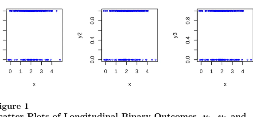
0 1 2 3 4 0.0 0.4 0.8 x y1 0 1 2 3 4 0.0 0.4 0.8 x y2 0 1 2 3 4 0.0 0.4 0.8 x y3 Figure 1
Scatter Plots of Longitudinal Binary Outcomes, y1, y2 and
y3, Against Covariate x, with no Outliers
Figure 1 exhibits representative scatter plots of the longitudinal binary outcomes,
y1, y2 and y3, over three observation times (t = 1,2,3), against the covariate x
when the data are generated from the multivariate binary model (33) under an exchangeable correlation structure with α = 0.4. As expected, the missing data occurred at the second and third observation times for lower values ofxandy.
The proposed RPL estimates of the regression parameters (β0, β1, β2) and the nuisance parameters (τ0, τ1, τ2) of the missing data model were obtained from the iterative equations (27) and (31) using the tuning constantsc= 1.2 for the Huber’s psi functionψc(r), andγ0= 2 for the weight functionwas defined in (16). Typically,
these tuning constants are chosen so as to provide a certain level efficiency at the underlying distributions. However, it is difficult to obtain an optimal set of values for the tuning constants analytically due to the complex nature of the robust estimators under incomplete binary data. We explore different sets of tuning constants for the RPL estimators and finally chose the valuesc= 1.2 andγ0= 2 for which the RPL
estimators of the regression parameters provided roughly 95% efficiency over the ordinary pseudo-likelihood (IPL) estimators under correctly specified models. Note that for the choicec =∞ andγ0= 0, the RPL estimators lead to the non-robust IPL estimators.
Table 1
Empirical Biases of RPL and IPL Estimators for Data with no Outliers
Parameter True Independent Exchangeable Serial value α= 0.2 α= 0.4 α= 0.2 α= 0.4 Robust method (RPL)
β0 0.50 0.0184 0.0095 0.0004 –0.0057 0.0048
β1 0.25 –0.0037 0.0012 0.0063 0.0079 0.0007
β2 –0.25 0.0060 0.0036 –0.0029 –0.0121 0.0088
Classical method (IPL)
β0 0.50 0.0194 0.0093 0.0017 0.0027 0.0008
β1 0.25 –0.0035 0.0014 0.0059 0.0044 0.0033
β2 –0.25 0.0070 0.0026 –0.0017 –0.0093 0.0061
Table 1 presents the empirical biases of both the RPL and IPL estimators un-der different correlation structures. It is clear from the table that both methods provide roughly unbiased estimators of the regression parameters β0, β1 and β2. Tables 2 presents the empirical mean squared errors of the RPL and IPL estima-tors. The RPL method appears to lose small efficiency in terms of slightly larger mean squared errors of the regression estimators. For example, under the correctly specified “independent” model, the RPL estimator ofβ1 is 92.2% as efficient as the corresponding IPL estimator; under the exchangeable correlation withα= 0.2, the efficiency of the RPL estimator of β1 is 96.6%. Also, under the serial correlation
withα= 0.4, the efficiency of the RPL estimator of β1 is 93.4%. We would expect
to lose such small efficiencies from the robust method when there are, in fact, no outliers in the data. However, our focus is on the robust analysis of data in the pres-ence of outliers. In the next step, we investigate the performance of the estimators under outliers.
We ran the second set of simulations by contaminating the data with a small proportion of outliers. As before, a series of 1000 data sets, each of size N = 200, were generated from the multivariate binary model (33). The values of the binary random variablevit were generated from the missing data model (34). Note
that in the case of binary responses, outliers in the data can arise only through the design points x. After generating each data set, we created a few outliers by randomly moving a small proportion of the design points from the bulk of the data. Specifically, to create these outliers, we randomly replaced 5% of thexvalues in the original data by x+ 5. This type of contamination generally produces mean-shift outliers in the data. Figure 2 exhibits representative scatter plots of the longitudinal binary outcomes, y1, y2 and y3, over three observation times (t = 1,2,3), against the covariate x when data are contaminated with design outliers. In these plots, the outliers are indicated by the large values of the covariatexfor which the values ofy are 0.
Table 2
Empirical Mean Squared Errors of RPL and IPL Estimators for Data with no Outliers
Parameter True Independent Exchangeable Serial value α= 0.2 α= 0.4 α= 0.2 α= 0.4 Robust method (RPL)
β0 0.50 0.1045 0.1071 0.1200 0.1075 0.1282
β1 0.25 0.0180 0.0205 0.0246 0.0210 0.0244
β2 –0.25 0.0431 0.0367 0.0319 0.0428 0.0387
Classical method (IPL)
β0 0.50 0.0967 0.1036 0.1127 0.1020 0.1179 β1 0.25 0.0166 0.0198 0.0229 0.0199 0.0228 β2 –0.25 0.0405 0.0338 0.0299 0.0410 0.0362 0 2 4 6 8 0.0 0.4 0.8 x y1 0 2 4 6 8 0.0 0.4 0.8 x y2 0 2 4 6 8 0.0 0.4 0.8 x y3 Figure 2
Scatter Plots of Longitudinal Binary Outcomes, y1, y2 and
y3, Against Covariate xfor Data Contaminated with Design
Outliers
Table 3
Empirical Biases of RPL and IPL Estimators for Data with Outliers
Parameter True Independent Exchangeable Serial value α= 0.2 α= 0.4 α= 0.2 α= 0.4 Robust method (RPL)
β0 0.50 0.0948 0.0910 0.0948 0.0873 0.0839
β1 0.25 –0.0436 –0.0429 –0.0446 –0.0395 –0.0389
β2 –0.25 0.0404 0.0407 0.0253 0.0440 0.0387
Classical method (IPL)
β0 0.50 0.2725 0.2746 0.2676 0.2678 0.2639
β1 0.25 –0.1401 –0.1417 –0.1376 –0.1371 –0.1353
Table 3 presents the empirical biases of the RPL and IPL estimators for data under design outliers. It is clear from the table that the ordinary IPL estimators of the regression parameters generally produce much larger biases, as compared to the RPL estimators. For example, under independence, the RPL estimator of β1
produces a small bias of−0.0436, whereas the IPL estimator ofβ1produces a much larger bias of −0.1401. Also, as clear from Table 4, the empirical mean squared errors of the IPL estimators are almost uniformly larger than those of the RPL estimators. For example, under independence, the RPL estimator ofβ1has a mean squared error of 0.0195, whereas the IPL estimator ofβ1has a larger mean squared error of 0.0288. This demonstrates the usefulness of the proposed robust method in bounding the influence of potential outliers in the data.
Table 4
Empirical Mean Squared Errors of RPL and IPL Estimators for Data with Outliers
Parameter True Independent Exchangeable Serial value α= 0.2 α= 0.4 α= 0.2 α= 0.4 Robust method (RPL)
β0 0.50 0.1109 0.1216 0.1348 0.1196 0.1227
β1 0.25 0.0195 0.0220 0.0254 0.0214 0.0224
β2 –0.25 0.0437 0.0350 0.0290 0.0451 0.0393
Classical method (IPL)
β0 0.50 0.1468 0.1552 0.1608 0.1500 0.1524
β1 0.25 0.0288 0.0311 0.0314 0.0295 0.0305
β2 –0.25 0.0416 0.0346 0.0284 0.0430 0.0356
6. APPLICATION: ANALYSIS OF AIDS DATA
Here we present an analysis of the CD4 count data from the AIDS clinical trials described in the Introduction. The parameters are estimated by using the proposed robust approach, and Troxelet al.’s (1998) independent pseudo-likelihood approach under the assumption of nonignorable missingness.
Our study involves 431 patients who were diagnosed with AIDS or AIDS-related complex. All patients were observed at the baseline period t = 0. Among the predictors considered in the study, “Azt” is defined to be 1 if a patient is random-ized to treatment Azt, and 0 if he/she is randomrandom-ized to treatment Ddi; “Age” is defined to be 1 if the patient is 35 or older at baseline period, and 0 otherwise; and “BaseCD4” is defined as BaseCD4 =√baseline CD4 count/10. Note that since the covariates Azt and Age are both binary, any outliers in the data can arise only through the covariate BaseCD4. Figure 3 displays the histogram of the observed values of BaseCD4 and the corresponding scatter plot of weights w used in our robust analysis. The right tail area of the histogram indicates some extreme values in BaseCD4, which are downweighted by the weight function w, as shown in the scatter plot on the right panel.
Baseline CD4 counts Frequency 0.0 0.5 1.0 1.5 2.0 2.5 3.0 0 5 0 100 150 0 100 200 300 400 0.4 0.6 0.8 1.0 Patient Weight Figure 3
Histogram of Baseline CD4 Counts (BaseCD4) and Corresponding Scatter Plot of Weights wUsed in Robust Analysis. Design Outliers Are Indicated by Small Weights
In this study, the response of interest is normal CD4 cell count (>200 cells per cubic millimeter) versus abnormal CD4 cell count (≤200) measured at every week for up to 5 weeks from baseline (t=1, . . . , 5); the outcome is defined as yit = 1
if the CD4 count exceeds 200 and 0 otherwise. The cutoff of 200 cells per cubic millimeter was chosen because of its strong predictive value for the development of opportunistic infections, and has been adopted as a standard threshold of clinical importance. The main question of scientific interest is the effect of treatment on changes in CD4 cell count sufficiency over time.
We model the “success probability”, pit = P(yit = 1), as a function of the
covariates using the logistic regression:
logit(pit) =β0+β1BaseCD4i+β2Agei+β3Azti+β4t,
for t= 1, ...,5. We also model the probability of being observed at each follow-up time assuming that CD4 count is nonignorably missing since sicker patients may be more likely to come in for a further GP visit, e.g., sicker patients may have been hospitalized. We consider the missing data model:
logit(πit) = logit{P(vit= 1|xit, yit,τ)}
=τ0+τ1BaseCD4i+τ2Agei+τ3Azti+τ4t+τ5yit,
fort= 1, ...,5. Table 5 reports the RPL and IPL estimates of the model parameters with their approximate standard errors and corresponding z values. The RPL and IPL estimates appear to be generally close to each other for the regression parameters. However, the standard errors of the two sets of estimators are different to some extent. For example, the RPL estimator of the intercept term β0 has a standard error of 1.2048, whereas the IPL estimator has a standard error of 0.9014; for β1, the RPL and MPL methods provide standard errors of 0.7714 and 0.6073,
the fact that when there are outliers in the data in one direction (that is, when the outlying residuals are either all positives or all negatives), an ordinary non-robust method generally underestimates the standard errors.
From the robust analysis of the data, the CD4 counts appear to decrease over time. But there is no evidence of treatment effects, which indicates that the effects of the two treatments Azt and Ddi are not significantly different. The estimates of the parameters of the missing data model from the two methods are similar. The probability of a response decreases over time under both methods. This probability, however, increases when possibly unobserved responsey increases from 0 to 1.
Table 5
Analysis of AIDS Data
Variable RPL IPL
Estimate Std
error z value Estimate
Std error z value Regression model Intercept (β0) –10.3243 1.2048 –8.570 –9.6419 0.9014 –10.696 BaseCD4 (β1) 6.5015 0.7714 8.428 6.2027 0.6073 10.213 Age (β2) 1.4716 0.4028 3.654 1.0772 0.3663 2.941 Azt (β3) 0.1351 0.4128 0.327 0.4751 0.3491 1.361 Time (β4) –0.2254 0.0794 –2.840 –0.2330 0.0749 –3.110
Missing data model
Intercept (τ0) 1.4484 0.2493 5.810 1.4415 0.2487 5.795 BaseCD4 (τ1) 1.0552 0.3095 3.409 1.0796 0.3140 3.438 Age (τ2) –0.2596 0.1685 –1.541 –0.1835 0.1638 –1.120 Azt (τ3) –0.0960 0.1737 –0.553 –0.0956 0.1692 –0.565 Time (τ4) –0.3107 0.0345 –8.995 –0.3196 0.0352 –9.075 y(τ5) 1.3475 1.6650 0.809 0.3581 0.8467 0.423
We also investigate the residuals from the robust fit to identify any outliers in the data. Figure 4 displays scatter plots of the standardized residuals (yit−
ˆ
pit)/
p
ˆ
pit(1−pˆit) for the observed data at the time-points t = 1, . . . ,5. These
plots show some large residuals at each time-point, which may have influenced the ordinary IPL estimates and their standard errors.
0 200 400 0 5 10 15 t=1 Index residual 0 200 400 −10 0 5 15 t=2 Index residual 0 200 400 −10 0 5 t=3 Index residual 0 200 400 −5 0 5 10 t=4 Index residual 0 200 400 −4 0 4 8 t=5 Index residual Figure 4
Standardized Residuals from the Robust Analysis of AIDS Data
7. DISCUSSION
We have developed the proposed RPL method to provide protection against outliers in the data. We have briefly studied the asymptotic properties of the RPL estima-tors. The empirical properties of these estimators were studied in simulations. The simulation results indicate that the RPL method is almost as efficient as the IPL method for data with no outliers. But the gain in efficiency from this robust method is generally large when data are contaminated with outliers.
In the case of binary longitudinal data, no outliers are desired in the binary responses. But still outliers can arise in the standardized residuals as these can be arbitrarily large even for a binary model. The proposed robust method can be used to bound the influence of both outliers in the residuals and leverage points in the design space.
Note that for data with nonignorable missing responses, we assumed an indepen-dent binary logistic model to describe the missing data mechanism. It is, however, not clear how the robust estimators would behave under a misspecified missing data model. A sensitivity analysis could be performed to investigate the effects model misspecification. Work remains to be done in this direction.
ACKNOWLEDGMENTS
The author is grateful for the support provided by a grant from the Natural Sciences and Engineering Research Council of Canada.
REFERENCES
[1] Bahadur, R.R. (1961). A representation of the joint distribution of responses to n dichotomous items. In H. Solomon (Ed.), Studies in item analysis and prediction(pp. 158–68). Stanford University Press.
[2] Brown, C.H. (1990). Protecting against nonrandomly missing data in longi-tudinal studies. Biometrics, 46, 143–157.
[3] Cantoni, E., & Ronchetti, E. (2001). Robust inference for generalized linear models. Journal of the American Statistical Association, 96, 1022–1030. [4] Dantan, E., Proust-Lima, C., Letenneur, L., & Jacqmin-Gadda, H. (2008).
Pattern mixture models and latent class models for the analysis of multivariate longitudinal data with informative dropouts. The International Journal of Biostatistics, 4, article 14.
[5] Diggle, P., & Kenward, M.G. (1994). Informative dropout in longitudinal data analysis (with discussion). Applied Statistics, 43, 49–94.
[6] Finkelstein, D.M., Williams, P.L., Molenberghs, G., Feinberg, J., Powderly, W., Kahn, J., Dolins, R., & Cotton, D. (1996). Patterns of opportunistic infec-tions in patients with HIV infection. Journal of Acquired Immune Deficiency Syndromes and Human Retrovirology, 12, 38–45.
[7] Gallant, J.E., Moore, R.D., Richman, D.D., Keruly, J., & Chaisson, R.E. (1992). Incidence and natural history of cytomegalovirus disease in patients with advanced human immunodeficiency virus disease treated with zidovudine. Journal of Infectious Diseases, 166, 1223–1227.
gener-alized linear mixed models when the missing data mechanism is nonignorable. Biometrika, 88, 551–564.
[9] Ibrahim, J.G., Lipsitz, S. R., & Chen, M.H. (1999). Missing covariates in generalized linear models when the missing data mechanism is non-ignorable. Journal of the Royal Statistical Society (Ser. B), 61, 173–190.
[10] Kahn, J.O., Lagakos, S.W., & Richman, D.D. (1992). A controlled trial comparing continued zidovudine with didanosine in human immunodeficiency virus infection. New England Journal of Medicine, 327, 581–587.
[11] Le Cessie, & Van Houwelingen, J.C. (1994). Logistic regression for correlated binary data. Applied Statistics, 43, 95–108.
[12] Liang, K.-Y., & Zeger, S.L. (1986). Longitudinal data analysis using general-ized linear models. Biometrika, 73, 13–22.
[13] Little, R.J.A., & Rubin, D.B. (2002). Statistical analysis with missing data (2nd ed.). New Jersey: John Wiley & Sons.
[14] Meester, S.G., & MacKay, J. (1994). A parametric model for cluster correlated categorical data. Biometrics, 50, 954–963.
[15] Molenberghs, G., & Lesaffre, E. (1994). Marginal modelling of correlated or-dinal data using a multivariate Plackett distribution. Journal of the American Statistical Association, 89, 633–644.
[16] Plackett, R.M. (1965). A class of bivariate distributions. Journal of the Amer-ican Statistical Association, 60, 516–522.
[17] Preisser, J.S., & Qaqish, B.F. (1999). Robust regression to clustered data with application to binary responses. Biometrics, 55, 574–579.
[18] Robins, J.M., Rotnitzky, A., & Zhao, L.P. (1995). Analysis of semiparamet-ric regression models for repeated outcomes in the presence of missing data. Journal of the American Statistical Association, 90, 106–121.
[19] Prentice, R.L. (1988). Correlated binary regression with covariates specific to each binary observation. Biometrics, 44, 1033–1048.
[20] Rousseeuw, P.J., & van Zomeren, B.C. (1990). Unmasking multivariate out-liers and leverage points. Journal of the American Statistical Association, 85, 633–639.
[21] Sinha, S.K. (2004). Robust analysis of generalized linear mixed models. Jour-nal of the American Statistical Association, 99, 451–460.
[22] Sinha, S.K. (2008). Robust methods for generalized linear models with non-ignorable missing covariates. The Canadian Journal of Statistics, 36(2), 277– 299.
[23] Sinha, S.K., Laird, N.M., & Fitzmaurice, G.M. (2010). Multivariate logistic regression with incomplete covariate and auxiliary information. Journal of Multivariate Analysis, 101, 2389–2397.
[24] Sinha, S.K., Troxel, A. B., Lipsitz, S.R., Sinha, D., Fitzmaurice, G.M., Molen-berghs, G., & Ibrahim, J.G. (2011). A bivariate pseudo-likelihood for incom-plete longitudinal binary data with nonignorable non-monotone missingness. Biometrics, 67, 1119–1126.
[25] Troxel, A.B., Lipsitz, S.R., & Harrington, D.P. (1998). Marginal models for the analysis of longitudinal measurements subject to nonignorable non-monotone missing data. Biometrika, 85, 661–672.
[26] White, H. (1982). Maximum likelihood estimation of misspecified models. Econometrica, 50, 1–26.