Divisive hierarchical maximum likelihood clustering

(1)

R E S E A R C H

Open Access

Divisive hierarchical maximum likelihood

clustering

Alok Sharma

1,2,3

, Yosvany López

1,4

and Tatsuhiko Tsunoda

1,4,5*

From16th International Conference on Bioinformatics (InCoB 2017) Shenzhen, China. 20-22 September 2017

Abstract

Background:Biological data comprises various topologies or a mixture of forms, which makes its analysis extremely complicated. With this data increasing in a daily basis, the design and development of efficient and accurate statistical methods has become absolutely necessary. Specific analyses, such as those related to genome-wide association studies and multi-omics information, are often aimed at clustering sub-conditions of cancers and other diseases. Hierarchical clustering methods, which can be categorized into agglomerative and divisive, have been widely used in such situations. However, unlike agglomerative methods divisive clustering approaches have consistently proved to be computationally expensive.

Results:The proposed clustering algorithm (DRAGON) was verified on mutation and microarray data, and was gauged against standard clustering methods in the literature. Its validation included synthetic and significant biological data. When validated on mixed-lineage leukemia data, DRAGON achieved the highest clustering accuracy with data of four different dimensions. Consequently, DRAGON outperformed previous methods with 3-,4- and 5-dimensional acute leukemia data. When tested on mutation data, DRAGON achieved the best performance with 2-dimensional information.

Conclusions:This work proposes a computationally efficient divisive hierarchical clustering method, which can compete equally with agglomerative approaches. The proposed method turned out to correctly cluster data with distinct topologies. A MATLAB implementation can be extraced from http://www.riken.jp/en/research/labs/ims/ med_sci_math/ or http://www.alok-ai-lab.com

Keywords:Divisive approach, Hierarchical clustering, Maximum likelihood

Background

In unsupervised clustering algorithms, the class label or the state of nature of a sample is unknown. The partition-ing of data is then driven by considerpartition-ing similarity or distance measures. In some applications (e.g. genome-wide association studies, multi-omics data analyses), the number of clusters also remains unknown. Because such biological information usually tends to follow a normal

distribution, the distribution of samples of each cluster can be assumed to be Gaussian.

Hierarchical clustering methods, which can be mainly categorized into agglomerative (bottom-up) and divisive (top-down) procedures, are well known [1–20]. In ag-glomerative procedures, each sample is initially assumed to be a cluster. The two nearest clusters (based on a distance measure or criterion function) are then merged at a time. This merger continues until all the samples are clustered into one group. Consequently, a tree like structure known as dendrogram is yielded. If the num-ber of clusters is provided, the process of amalgamation of clusters can be terminated when the desired number of clusters is obtained. The first step of an agglomerative procedure considers all the possible mergers of two

* Correspondence:[email protected] 1

Laboratory for Medical Science Mathematics, RIKEN Center for Integrative Medical Sciences, Yokohama, Kanagawa 230-0045, Japan

4_{Department of Medical Science Mathematics, Medical Research Institute,} Tokyo Medical and Dental University, Tokyo 113-8510, Japan

Full list of author information is available at the end of the article

© The Author(s). 2017Open AccessThis article is distributed under the terms of the Creative Commons Attribution 4.0 International License (http://creativecommons.org/licenses/by/4.0/), which permits unrestricted use, distribution, and reproduction in any medium, provided you give appropriate credit to the original author(s) and the source, provide a link to the Creative Commons license, and indicate if changes were made. The Creative Commons Public Domain Dedication waiver (http://creativecommons.org/publicdomain/zero/1.0/) applies to the data made available in this article, unless otherwise stated.

(2)

samples, which requires n(n−1)/2 combinations (where

n depicts the number of samples). Divisive procedures, on the other hand, perform clustering in an inverse way as compared to their agglomerative counterparts. They begin by considering a group (having all the samples) and divide it into two groups at each stage until all the groups comprise of only a single sample [21, 22]. In the first step of a divisive procedure all the partitions of a sample set are considered, which amounts to 2n−1−1 combinations. This number of combinations grows exponentially and practically makes divisive clustering a difficult procedure to implement. However, there are a few divisive approaches which do not necessarily con-sider all the divisions [21]. In hierarchical classifications, each subcluster can be formed from one larger cluster split into two, or the union of two smaller clusters. In either case, false decisions made in early stages cannot be corrected later on. For this reason, divisive proce-dures, which start with the entire dataset, are in general considered safer than agglomerative approaches [21, 23]. Therefore, the accuracy of a divisive procedure is envisaged to be higher than that of an agglomerative procedure [24]. However, the high computational de-mand (O(2n)~O(n5)) of divisive procedures has severely restricted their usage [24, 25] (though for special cases the complexity can be further reduced [26]). Therefore, the divisive procedure has not been generally used for hierarchical clustering, remaining largely ignored in the literature.

Hierarchical approaches do not require initial param-eter settings and generally employed either linear or non-linear regression models [27–29]. Over the last few decades, a number of hierarchical approaches have been proposed. Some of these popular schemes are summa-rized below. The single linkage or link agglomerative hierarchical approach (SLink) [30] merges two adjacent neighbour groups. Euclidean distance for computing the proximity between two clusters. SLink is very sensitive to data location and occasionally generates groups in a long chain (called as chaining effect). This chaining effect can be reduced developing a method based on farthest distance. This was achieved by the complete linkage (CLink) hierarchical approach [2]. Nevertheless, CLink is also sensitive to outliers. Sensitiveness could be further decreased by the average linkage (ALink) hier-archical approach [31, 32]. ALink implements linking by using the average distance between two groups. In a similar way, the median linkage (MLink) hierarchical approach [33] regards median distance for linking. In Ward’s linkage (Wa-Link), clusters are merged based on the optimal value of an objective function [34]. In weighted average distance linkage (Wt-Link) hierarchical clustering [35, 36], the group sizes are not considered when computing average distances. Consequently,

smaller groups will be assigned larger weights during the clustering process [35]. Similarly, model-based hierarch-ical clustering [4, 8] uses an objective function. Whereas the method in [8] follows a Bayesian analysis and uses both Dirichlet priors and multinomial likelihood func-tion, the approach in [4] optimizes the distance between two GMMs. The number of group is previously defined. Most of these approaches are constructed using the agglomerative procedure, though their construction (with higher computational demand) is equally possible using the divisive procedure. Although divisive cluster-ing is generally disregarded, some approaches like DIANA (DIvisive ANAlysis) program has been recently established [21]. In spite of well-established methods (i.e. EM algorithm [37, 38]) for estimating the parameters of a Gaussian mixture model, it is worth noting that hier-archical and expectation-maximization (EM) algorithms are very different in nature. The EM algorithm is an iterative optimization method, which requires prior knowledge of the number of clusters. It begins with a random choice of cluster centers and therefore returns different sets of clusters for distinct runs of the algo-rithm. Hierarchical clustering algorithms, on the other hand, do not require such prior knowledge and return a unique set of clusters. These advantages often make hierarchical clustering methods preferable to the EM algorithm for dealing with biological datasets where unique solutions are of utmost importance [39–41].

In this work, we described a new Divisive hieRArchical maximum likelihOod clusteriNg approach, abbreviated as DRAGON hereafter. This is a top-down procedure which does not find pairs. Instead, it takes out one sample at a time, maximally increasing the likelihood function. This process continues until the first cluster is obtained. This cluster is not further subdivided but removed from the sample set. In the remaining sample set, the same procedure is repeated for obtaining all the possible clusters. The removal of one sample out of n

samples requires nsearch. This reduces the total search complexity toO(n2c) (wherecis the number of clusters), which represents a significant reduction of the top-down procedure. The following sections present the mathem-atical derivation of the proposed model, and the analyses carried over on synthetic as well as on biological data to illustrate its usefulness.

Methods

Maximum likelihood clustering: an overview

This section summarizes an overview of the maximum likelihood method for clustering [22]. Here we are not introducing our method, instead we are proving a brief description of conventional maximum likelihood ap-proach for clustering applications. It is possible to learn from an unlabeled data if some assumptions are taken.

(3)

We will begin the section with an assumption that prob-ability densities are known and it is required to estimate unknown parametric vector θ. The solution comes out to be similar to supervised learning case of maximum likelihood estimation. However, in the supervised learn-ing case, the topology of groups of data is known. But in an unsupervised learning case one has to assume para-metric form of data to reach to the solution. Here we describe how to estimate of maximum likelihood of clus-ters of a given sample set χ. The label of cluster of the sample sets is defined as ω. Assuming there are c clus-ters in the sample set (c≥1), we define Ω= {ωj} (for j=

1, 2,…,c) as the cluster label forjth clusterχj(In many

clustering problems, the number of c is unknown, this issue we will deal in detail in later section and in Additional file 1). In this paper, we followed the nota-tions from Duda et al. [22] for the convenience of readers. Let a sample set χ= {x1,x2,…,xn} be defined in

ad-dimensional space (It is assumed thatd<n. Ford≫ n, dimensionality reduction techniques can be first applied for supervised or unsupervised learning tasks [42–47]). Let an unknown parameter vector be θ consisting of mean μ as well as covariance Σ. This will specify the mixture density as

pðxkjθÞ ¼Xc

j¼1p xkjωj;θj

P ωj ð1Þ

wherep(xk|ωj,θj) (forj= 1,…,c) is the conditional dens-ity,P(ωj) is the a priori probability andθ= {θj}. The joint density is further defined using the log likelihood as

L¼ logpðχjθÞ ¼ logYn

k¼1pðxkjθÞ

¼Xn_k_¼₁logpðxkjθÞ ð2Þ

Assuming the joint densityp(χ|θ) is differentiable w.r.t toθthen from Eqs. (1) to (2)

∇θiL¼ Xn k¼1 1 pðxkjθÞ∇θi Xc j¼1p xkjωj;θj P ωj h i ð3Þ where ∇θiL is the gradient of L w.r.t. θi. Assuming θi

andθjare independent, and supposing a posteriori prob-ability is

Pðωijxk;θÞ ¼

pðxkjωi;θiÞPð Þωi

pðxkjθÞ ð4Þ

then from Eq. (4) we can observe that 1 pðxkjθÞ¼

Pðωijxk;θÞ

pðxkjωi;θiÞPð Þωi. Substituting this value in Eq. (3), we obtain ∇θiL¼

Xn

k¼1Pðωijxk;θÞ∇θilogpðxkjωi;θiÞ ð5Þ

Note that in Eq. (5), (1/f(z))∇zf(z) is arranged as∇zlog

f(z). Equation (5) can be equated to 0 (∇θiL¼0 ) for obtaining maximum likelihood estimateθ^i. This will give

us the solution as (interested readers may refer to Duda et al. [22] for further details.)

Pð Þ ¼ωi 1 n Xn k¼1P ωijxk;^θ ð6Þ Xn k¼1P ωijxk;^θ ∇θilogp xkjωi;θ^i ¼0 ð7Þ P ωijxk;θ^ ¼ p xkjωi;θ^i Pð Þωi Pc j¼1p xkjωj;^θj P ωj ð8Þ In the case of normal distribution, the unknown mean and covariance {μ,Σ} parameters are replaced inθin the Eqs. 6, 7 and 8 for yielding maximum likelihood esti-mates. The parameterθis usually updated in an iterative fashion to attain θ^ by EM algorithms or hill climbing schemes.

DRAGON method: concept

Here we illustrate the clustering method DRAGON. In brief, the proposed procedure is top-down in nature. It initially considers the sample set as one cluster from which one sample is removed at a time. This increases the likelihood function and continues until the max-imum likelihood is reached as depicted in Fig. 1 (where

L1 is the cluster likelihood at the beginning of the process and L3is the maximum likelihood after remov-ing two samples). Once the first cluster is obtained it is removed from the sample set and the procedure is then repeated for attaining the subsequent clusters. Conse-quently, only one cluster will be retrieved from a sample set. It is assumed that samples are multinomial distrib-uted, however, the number of clusters is not known at the beginning of the process.

Fig. 1An illustration of the DRAGON method. This procedure results in the formation of one cluster. One sample is removed at a time, which maximally increases the likelihood function. At the beginning, the likelihood wasL1and after two iterations the likelihood became

(4)

To establish the maximum likelihood estimate in the divisive hierarchical context, we investigate the criterion function and the distance measure that satisfy it.

DRAGON method: algorithm

To find the distance measure, we first define the log-likelihood function of a clusterχs, whereχsis a subset of

χ. At the beginning,χsis the same asχ, however, in every

subsequent iteration a samplex is removed fromχssuch

that the likelihood function

L¼X_x_∈_χ s

log½pðxjω;θÞPð Þω ð9Þ is maximized.

Since we are finding only one cluster in the sample set χ, a priori probability P(ω) can be ignored. We would like to explore how functionLchanges when a sample^x is taken out. Let us suppose centroidμand covarianceΣ ofχsare defined as μ¼1 n X x∈χsx ð 10Þ Σ¼1 n X x∈χsðx−μÞðx−μÞ T _ð 11Þ where the number of samples in χs is depicted as n. Assuming that the component density is normal then Eq. (9) can be simplified as

L¼P_x_∈_χ slog 1 2π ð Þd=2 Σ j j1=2_exp ₋1 2ðx−μÞ T_Σ−1_ð_x−_μ_Þ 2 4 3 5 2 6 6 4 3 7 7 5 ¼−1 2tr Σ −1X x∈χsðx−μÞðx−μÞ T h i −nd 2 log2π− n 2logj jΣ where trace function is denoted by tr(). Since tr

Σ−1P x∈χsðx−μÞðx−μÞ T h i ¼tr nIð ddÞ ¼nd, we can write Las L¼−1 2nd− nd 2 log2π− n 2logj jΣ ð12Þ If a sample ^x is removed from χs then centroid and

covariance (Eqs. (10) and (11)) will change as follows

μ_¼_μ₋^x−μ n−1 ð13Þ Σ_¼ n n−1Σ− n n−1 ð Þ2ð^x−μÞðx^−μÞ T _ð 14Þ In order to observe the alteration in the likelihood function (of Eq. (12)), we provide the following Lemma.

Lemma 1 Assume point ^x is taken out of a setχsand this changes the centroid and covariance (as Eqs. (13)

and (14) described). Thereby the determinant of Σ* is defined as Σ j j ¼ n n−1 d Σ j j 1− 1 n−1ðx^−μÞ T_Σ−1_ð_^_x₋_μ_Þ

ProofFrom Eq. (14), the determinant ofΣ*will be Σ j j ¼ n n−1Σ− n n−1 ð Þ2ðx^−μÞðx^−μÞ T ðL1Þ

For any square matrix of size m×m, we can write |AB| = |A||B|, and |cA| =cm|A| where c is any scalar, This would enable us to write Eq. (L1) in the following manner Σ j j ¼ n n−1 d Σ j jIdd− 1 n−1ðx^−μÞð^x−μÞ T_Σ−1 ðL2Þ ImmþAB j j can be proved to be |In×n+BA| by

Sylvester’s determinant theorem (where A∈ℝm×n and

B∈ℝn×mare rectangular matrices). This would allow us to write Idd− 1 n−1ð^x−μÞðx^−μÞ T_Σ−1 ¼ 1− 1 n−1ðx^−μÞ T_Σ−1_ð_^_x₋_μ_Þ

For any scalar |c| =c, the Lemma is then proved by substituting this term in Eq. (L1).□

It is now possible to define the change inLas

L¼L−ΔL ð15Þ whereΔLis defined as ΔL¼−1 2 logj j þΣ n−1 2 log 1− P n−1 þn−1 2 dlog n n−1− d 2− d 2 log2π ð16Þ andPis expressed as P¼ðx^−μÞTΣ−1_ð_x_^₋_μ_Þ _ð₁₇_Þ It can be observed from Eqs. (15) to (17) that when a sample x^ is taken out of cluster χs, the change in L

mainly depends on the termPas all the other terms are not changing. If we want to selectx such thatL*>L, this requires to solve the following maximization problem

^

x¼ arg maxx∈χsP ð18Þ

Therefore, by removing ^x the likelihood should increase until the maximum value is reached.

This procedure can track the location of the cluster having the highest density or likelihood. Because one

(5)

sample is taken out at a time, it could be sensitive to data positions around the center of the cluster. Thereby, it is possible to locate the center of the cluster whereas its complete topology can be missed. In order to reduce such sensitiveness additional processing for tuning the cluster would be useful.

By taking out one sample at a time, we can obtain a cluster χs that provides maximum likelihood. All the

samples taken out can be collated in a set defined asχ_s, where χ_s∪χ_s ¼χ. The centroid of cluster χs can be

obtained byμs=E[χs]. It can be then employed to

com-pute the distance of all the samples fromμs; i.e.dx=δ(x,

μs)∀x∈χ, where δ denotes a distance measure (in this

case the Euclidean metric) and dx is a 1-dimensional

sample or point corresponding to x. Thereafter, a centroid-based clustering scheme can be applied on this distance metric or inner product space (by considering 1-dimensional data and partitioning it into 2 groups) to readjust the cluster χs. Here clustering is applied on a

distance metric, which can be either the Euclidean norm or any form of kernel (as it is derived from dot product). This procedure can be repeated ifμsis changing

dramat-ically. The overall method is summarized in Table 1 and illustrated in Additional file 1 (slides 1–6).

The next issue is the estimation of the number of clus-ters (c). If the value of cwere given, it is then easier to find the locations. However, in some applications, c is unknown. In such situations, a range of values of ccan be inserted to the procedure so that the best value in the range can be estimated. If no clue about c were given, the maximum number of possible clusters C can be investigated and the best among them (c≤C) can be chosen. In order to estimate c, we first define the total likelihood function as

Ltð Þ ¼c Xc

i¼1Li ð19Þ

where Li is the likelihood of ith cluster. The total likeli-hood functionLtcan be computed for different values of

c. If for a particular number of clusters (k), the variation between two successive total likelihood functions were not significant, then we can estimatecto bek. Let the dif-ference between two successive total likelihoods beδLt(k) =Lt(k+ 1)−Lt(k), this quantity can be normalized as

δLt← δ

Lt−minðδLtÞ

maxðδLtÞ−minðδLtÞ ð 20Þ whereδLtis normalized over all the possible values ofk.

Figure S5 in Additional file 1 illustrates the above explanation with a dataset of 4 clusters.

DRAGON method: search complexity

In this section, we briefly discuss the search complexity of the DRAGON method. As explained above the proposed method begins by taking one sample out of the sample set, which increases the likelihood function and requires n

search. However, in the second iteration the search reduces to n−1. Finding a cluster having n1samples requires (1/ 2)(n−n1)(n+n1+ 1) total search (see Additional file 2 for details). Therefore, the search forcclusters resultsO(n2c). It should be noted here that this search in conventional divisive hierarchical approaches is quite expensive, in the order ofO(2n). However, the search of DRAGON is in the order of O(n2c), which indicates a considerable reduction. Furthermore, DRAGON employs the k-means clustering algorithm in the dot product space as an intermediate step. The computational complexity of k-means is considered to be linear (e.g. using Lloyd’s algorithm this isO(2nt) because dimensionality is 1 in an intermediate step, and the number of classes is 2. Here,trepresents the number of iterations).

Results and discussion

To validate the DRAGON method, we performed analyses using synthetic and biological data. We further compared its clustering accuracy with that of existing hierarchical methods.

Analysis on synthetic data

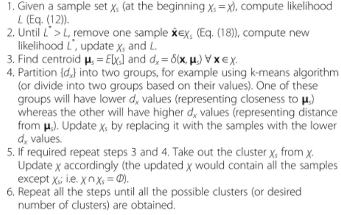
For the analysis on synthetic data, we generated Gauss-ian data of dimensionality d with 4 clusters. This data consisted of 400 samples with similar topology to that described in Figure S1 of Additional file 1). With the help of different random seeds we produced the data 20 times, and for on each occasion we calculated the clus-tering accuracy. We then computed the average or mean of clustering accuracy over 20 attempts to have a statisti-cally stable value. The dimension of the generated data was increased from 2 to 30. For evaluation purposes, we also used other agglomerative hierarchical methods such as SLink, CLink, MLink, ALink, Wa-Link, and Wt-Link. The average clustering accuracies of these approaches over dimensionality d are shown in Fig. 2a. For all the Table 1DRAGON Method

1. Given a sample setχs(at the beginningχs=χ), compute likelihood

L(Eq. (12)). 2. UntilL*_>

L, remove one sample^x∈χ_s(Eq. (18)), compute new likelihoodL*, updateχsandL.

3. Find centroidμs=E[χs] anddx=δ(x,μs)∀x∈χ.

4. Partition {dx} into two groups, for example using k-means algorithm (or divide into two groups based on their values). One of these groups will have lowerdxvalues (representing closeness toμs) whereas the other will have higherdxvalues (representing distance fromμs). Updateχsby replacing it with the samples with the lower

dxvalues.

5. If required repeat steps 3 and 4. Take out the clusterχsfromχ. Updateχaccordingly (the updatedχwould contain all the samples exceptχs; i.e.χ∩χs=Φ).

6. Repeat all the steps until all the possible clusters (or desired number of clusters) are obtained.

(6)

above methods, we provided the number of clusters; i.e.

c= 4. For the DRAGON method (of Table 1), we iterated two times (step 5 of Table 1) in all the experiments. Additionally, we assessed seven previously compared divisive hierarchical methods [24]: ALink (average link), SLink (single link), CLink (complete link), DunnsOrg (Dunn’s original), DunnsVar (Dunn’s variant), Mac-Smith (Macnaughton-Smith) and PDDP (Principal Direction). The average clustering accuracies of these divisive methods are summarized in Fig. 2b. As Fig. 2b shows when the dimensionality of data increases, Mac-Smith performs poorly whereas ALink, SLink and DunnsOrg slightly improve their performances. The data dimension did not affect the accuracy of DunnsVar whatsoever, which remains around 50%. The highest accuracy is achieved by the PDDP method (roughly 80%), however, this accuracy is still lower than that of DRAGON.

It can be observed from Fig. 2 that on Gaussian data, the DRAGON method provides promising results over other hierarchical methods either agglomerative or divisive. The Wa-Link hierarchical method also shows good results after the DRAGON method over dimen-sionalityd= 2,…, 30.

To avoid limiting our validation to Gaussian datasets, we carried out additional analyses on synthetic data that included Pathbased [48], Flame [49] and Aggregation [50] datasets. The results are summarized in Tables S1.1, S1.2 and S1.3 of Additional file 1.

Analysis on biological data

We also utilized biological datasets, namely acute leukemia [51], mixed-lineage leukemia (MLL) [52] and mutation data from The Cancer Genome Atlas for assessing clustering accuracy of several hierarchical approaches studied in this paper. A summary of datasets can be found below:

Acute leukemia dataset –comprises DNA microarray gene expressions. The samples belong to acute leukemias

of humans. Two kinds are available: acute myeloid leukemia (AML) and acute lymphoblastic leukemia (ALL). The dataset has 25 AML and 47 ALL bone marrow sam-ples with a dimension of 7129.

MLL dataset–has three ALL, MLL and AML classes. It contains 72 leukemia samples where 24 belong to ALL, 20 belong to MLL and 28 belong to AML with dimensionality 12,582.

Mutation dataset – this dataset is derived from The Cancer Genome Atlas project (https://tcga-data.nci.nih.-gov/docs/publications/tcga/?). It includes mutation data for breast cancer, glioblastoma, kidney cancer and ovar-ian cancer. The data is divided into two groups of 416 samples and 90 samples, which contain 1636 genes.

To vary its number of features or dimensions, we employed the Chi-squared method for ranking the genes (the InfoGain feature selection method was also Fig. 2Average clustering accuracy (over 20 attempts) on synthetic data with four clusters for (a) DRAGON and various agglomerative hierarchical methods, and (b) divisive hierarchical methods

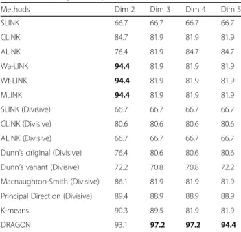
Table 2Clustering accuracy (%) on acute leukemia dataset

Methods Dim 2 Dim 3 Dim 4 Dim 5

SLINK 66.7 66.7 66.7 66.7 CLINK 84.7 81.9 81.9 81.9 ALINK 76.4 81.9 84.7 84.7 Wa-LINK 94.4 81.9 81.9 81.9 Wt-LINK 94.4 81.9 81.9 81.9 MLINK 94.4 81.9 81.9 81.9 SLINK (Divisive) 66.7 66.7 66.7 66.7 CLINK (Divisive) 80.6 80.6 80.6 80.6 ALINK (Divisive) 66.7 66.7 66.7 66.7

Dunn’s original (Divisive) 76.4 80.6 80.6 80.6 Dunn’s variant (Divisive) 72.2 70.8 70.8 72.2 Macnaughton-Smith (Divisive) 86.1 81.9 81.9 81.9 Principal Direction (Divisive) 89.4 88.9 88.9 88.9

K-means 90.3 89.5 81.9 81.9

(7)

employed, see Additional file 3). We then performed clustering on samples and computed the clustering accuracy on dimensionality d= 2, …, 5. The clustering accuracies (was measured with the package AccMeasure 2011: http://www.mathworks.com/matlabcentral/fileex-change/32197-clustering-results-measurement/content/ AccMeasure.m) on acute leukemia, MLL and muta-tion datasets are depicted in Tables 2, 3 and 4, respect-ively. The best outcomes are highlighted in bold faces.

It is noticed from Table 2 that Wa-Link, Wt-Link and MLink achieve the highest performance when d= 2. For the other dimensions (d= 3, 4 and 5), DRAGON shows

the highest performance. From Table 3, it can be seen that DRAGON achieves reasonable performance for all the dimensions. On mutation data (Table 4), DRAGON is showing the highest performance ford= 2 and slightly low performance (82.2%) for the other dimensions. Dunn’s original and Macnaughton-Smith provide the highest performance when d= 3. Despite the reasonable performance of divisive clustering methods in Table 4, it is worth noting that their running times were extremely slow, specially when the number of samples increases as it is the case with mutation data. In general, it can be summarized that the DRAGON method exhibited prom-ising results in terms of clustering accuracy over other hierarchical methods. Also its search complexity is

O(n2c), which is significantly lower than that of conven-tional divisive approaches.

Conclusions

In this work, we proposed a divisive hierarchical maximum likelihood clustering method whose search complexity was reduced toO(n2c). Its overall clustering accuracy showed a significant improvement over that of agglomerative hierarchical clustering methods when compared on both synthetic and biological datasets.

Additional files

Additional file 1:Divisive hierarchical maximum likelihood clustering. In this file an illustration of DRAGON method is given. Additionally, performance (in terms of Rand index) is given for synthetic data (Flame, Pathbased and Aggregation). (PDF 963 kb)

Additional file 2:Computational consideration of DRAGON search. In this file derivation of computational complexity of DRAGON search is given. (PDF 84 kb)

Additional file 3:Clustering accuracy using InfoGain feature selection method. In this file, InfoGain filtering method was used to perform feature selection. Thereafter, various clustering methods were used to evaluate the performance of DRAGON method. (PDF 68 kb)

Abbreviations

ALL:Acute lymphoblastic leukemia; AML: Acute myeloid leukemia; CLink: Complete linkage; DIANA: Divisive analysis; DRAGON: Divisive hierarchical maximum likelihood clustering; EM: Expectation-maximization; GMM: Gaussian mixture model; ML: Maximum likelihood; MLink: Median linkage; MLL: Mixed lineage leukemia; SLink: Single linkage; Wa-Link: Ward’s linkage; WLink: Weighted average distance linkage; Wt-Link: Weighted linkage

Acknowledgements

We thank Maurice Roux for kindly providing us with his implementation of divisive hierarchical clustering algorithms. High-end computing resources were provided by the Advanced Center for Computing and Communication, RIKEN.

Funding

This study was funded by the CREST, JST Grant, Japan. Availability of data and materials

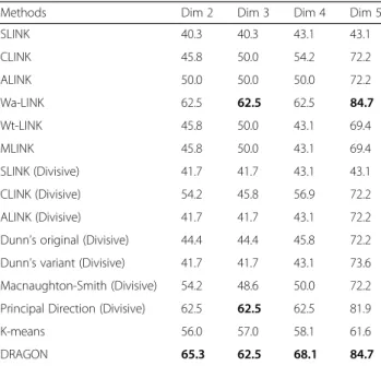
The ALL and MLL datasets are publicly accessible and can be downloaded via the author’s webpage or the Kent Ridge Biomedical Data Set Repository. The mutation data can be retrieved from The Cancer Genome Atlas Project. The MATLAB package of DRAGON can be accessed at http://www.riken.jp/ en/research/labs/ims/med_sci_math/ or http://www.alok-ai-lab.com Table 3Clustering accuracy (%) on MLL dataset

K-means 56.0 57.0 58.1 61.6

DRAGON 65.3 62.5 68.1 84.7

Table 4Clustering accuracy (%) on mutation dataset

K-means 64.9 67.1 65.7 63.3

(8)

Declarations

The publication charges of this article were funded by JST CREST grant JPMJCR1412.

About this supplement

This article has been published as part ofBMC BioinformaticsVolume 18 Supplement 16, 2017: 16th International Conference on Bioinformatics (InCoB 2017): Bioinformatics. The full contents of the supplement are available online at https://bmcbioinformatics.biomedcentral.com/articles/ supplements/volume-18-supplement-16.

Authors’contributions

AS developed the concept, conducted the experiments and wrote the first draft of the manuscript. YL carried out the experiments related to divisive hierarchical clustering and proofread the manuscript. TT supervised the entire project. All the authors read and approved the final manuscript. Ethics approval and consent to participate

None

Consent for publication Not applicable Competing interests

The authors declare that they have no competing interests.

Publisher’s Note

Springer Nature remains neutral with regard to jurisdictional claims in published maps and institutional affiliations.

Author details 1

Laboratory for Medical Science Mathematics, RIKEN Center for Integrative Medical Sciences, Yokohama, Kanagawa 230-0045, Japan.2_{Institute for} Integrated and Intelligent Systems, Griffith University, Brisbane, QLD 4111, Australia.3_{School of Engineering & Physics, University of the South Pacific,} Suva, Fiji.4Department of Medical Science Mathematics, Medical Research Institute, Tokyo Medical and Dental University, Tokyo 113-8510, Japan. 5_{CREST, JST, Tokyo 113-8510, Japan.}

Published: 28 December 2017 References

1. Castro RM, Coates MJ, Nowak RD. Likelihood based hierarchical clustering. IEEE Trans Signal Process. 2004;52(8):2308–21.

2. Defays D. An efficient algorithm for a complete link method. Comput J. 1977;20(4):364_–6.

3. Fisher D. Iterative optimization and simplification of hierarchical clusterings. J Artif Intell Res. 1996;4(1):147–79.

4. Goldberger J, Roweis S. Hierarchical clustering of a mixture model. In: Neural information processing systems. Cambridge: MIT Press; 2005. p. 505_–12. 5. Heller KA, Ghahramani Z. Bayesian hierarchical clustering. In: 22nd

international conference on machine learning. ACM: New York, Bonn; 2005. p. 297–304.

6. Horng S-J, M-Y S, Chen Y-H, Kao T-W, Chen R-J, Lai J-L, Perkasa CD. A novel intrusion detection system based on hierarchical clustering and support vector machines. Expert Syst Appl. 2011;38(1):306–13.

7. Jain AK, Murty MN, Flynn PJ. Data clustering: a review. ACM Comput Surv. 1999;31(3):264_–323.

8. Vaithyanathan S, Dom B. Model-based hierarchical clustering. In: 16th conference in uncertainty in artificial intelligence; 2000. p. 599–608. 9. Sharma A, Boroevich KA, Shigemizu D, Kamatani Y, Kubo M, Tsunoda T.

Hierarchical maximum likelihood clustering approach. IEEE Trans Biomed Eng. 2017;64(1):112–22.

10. Zhang W, Zhao D, Wang X. Agglomerative clustering via maximum incremental path integral. Pattern Recogn. 2013;46(11):3056–65. 11. Rokach L, Maimon O. Clustering methods. In: Maimon O, Rokach L, editors.

Data mining and knowledge discovery handbook. US: Springer; 2005. p. 321–52.

12. Székely GJ, Rizzo ML. Hierarchical clustering via joint between-within distances: extending Ward_’s minimum variance method. J Classif. 2005; 22:151–83.

13. Karypis G, Han E-H, Kumar V. Chameleon: hierarchical clustering using dynamic modeling. Computer. 1999;32(8):68_–75.

14. Murtagh F, Legendre P. Ward_’s hierarchical agglomerative clustering method: which algorithms implement ward’s criterion? J Classif. 2014;31(3):274–95. 15. Bouguettaya A, Yu Q, Liu X, Zhou X, Song A. Efficient agglomerative

hierarchical clustering. Expert Syst Appl Int J. 2015;42(5):2785–97. 16. Zhang X, Xu Z. Hesitant fuzzy agglomerative hierarchical clustering

algorithms. Int J Syst Sci. 2015;46(3):562_–76.

17. Murtagh F, Contreras P. Algorithms for hierarchical clustering: an overview. WIREs Data Min Knowl Discov. 2012;2(1):86–97.

18. Gómez D, Yáñez J, Guada C, Rodríguez JT, Montero J, Zarrazola E. Fuzzy image segmentation based upon hierarchical clustering. Knowl-Based Syst. 2015;87:26_–37.

19. Zhou G-T, Hwang SJ, Schmidt M, Sigal L, Mori G. Hierarchical maximum-margin clustering. Ithaca: Cornell University Library; 2015.

20. Wang J, Zhong J, Chen G, Li M, F-X W, Pan Y. ClusterViz: a cytoscape APP for cluster analysis of biological network. IEEE/ACM Trans Comput Biol Bioinform. 2015;12(4):815_–22.

21. Kaufman L, Rousseeuw PJ. Finding groups in data: an introduction to cluster analysis. 1st ed: Wiley-Interscience; Hoboken, New Jersey; 2005.

22. Duda RO, Hart PE, Stork DG. Pattern classification. 2nd ed: Wiley-Interscience; New York; 2000.

23. Macnaughton-Smith P, T Williams W B. Dale M G. Mockett L: Dissimilarity analysis: a new technique of hierarchical sub-division. Nature 1964, 202:1034-1035. 24. Roux M. A comparative study of divisive hierarchical clustering algorithms.

Ithaca: Cornell University Library; 2015.

25. Roux M. Basic procedures in hierarchical cluster analysis. In: Devillers J, Karcher W, editors. Applied multivariate analysis in SAR and environmental studies. Dordrecht: Springer Netherlands; 1991. p. 115_–35.

26. Guénoche A, Hansen P, Jaumard B. Efficient algorithms for divisive hierarchical clustering with the diameter criterion. J Classif. 1991;8(1):5–30. 27. Farrell S, Ludwig CJH. Bayesian and maximum likelihood estimation of

hierarchical response time models. Psychon Bull Rev. 2008;15(6):1209–17. 28. Pinheiro J, Bates D. Mixed-effects models in S and S-PLUS. 2000th ed. New

York: Springer; 2009.

29. Raudenbush SW, Bryk AS. Hierarchical linear models: applications and data analysis methods. 2nd ed. Thousand Oaks: SAGE Publications; 2001. 30. Sibson R. SLINK: an optimally efficient algorithm for the single-link cluster

method. Comput J. 1973;16(1):30–4.

31. Sokal RR, Michener CD. A statistical method for evaluating systematic relationships. Univ Kansas Sci Bull. 1958;38(22):1409–38.

32. Legendre P, Legendre L. Numerical Ecology. 3rd ed: Elsevier; 2012. 33. Everitt BS, Landau S, Leese M, Stahl D. Cluster analysis. 5th ed: Wiley; 2011. 34. Ward JH. Hierarchical grouping to optimize an objective function. J Am Stat

Assoc. 1963;58(301):236–44.

35. Podani J. Multivariate data analysis in ecology and systematics: SPB Academic Publishing; 1994.

36. McQuitty LL. Similarity analysis by reciprocal pairs for discrete and continuous data. Educ Psychol Meas. 1966;26(4):825_–31.

37. McLachlan G, Krishnan T. The EM algorithm and extensions. 2nd ed: Wiley-Interscience; 2008.

38. Jordan MI, Jacobs RA. Hierarchical mixtures of experts and the EM algorithm. Neural Comput. 1994;6(2):181–214.

39. González M, Gutiérrez C, Martínez R. Expectation-maximization algorithm for determining natural selection of Y-linked genes through two-sex branching processes. J Comput Biol. 2012;19(9):1015–26.

40. Do CB, Batzoglou S. What is the expectation maximization algorithm? Nat Biotechnol. 2008;26(8):897–9.

41. Holmes I. Using evolutionary expectation maximization to estimate indel rates. Bioinformatics. 2005;21(10):2294–300.

42. Sharma A, Paliwal KK. Fast principal component analysis using fixed-point algorithm. Pattern Recogn Lett. 2007;28(10):1151_–5.

43. Sharma A, Paliwal KK. A gradient linear discriminant analysis for small sample sized problem. Neural Process Lett. 2008;27(1):17–24.

44. Sharma A, Paliwal KK. Cancer classification by gradient LDA technique using microarray gene expression data. Data Knowl Eng. 2008;66(2):338–47. 45. Sharma A, Paliwal KK. Rotational linear discriminant analysis technique for

dimensionality reduction. IEEE Trans Knowl Data Eng. 2008;20(10):1336_–47. 46. Sharma A, Paliwal KK, Onwubolu GC. Class-dependent PCA, MDC and

LDA: a combined classifier for pattern classification. Pattern Recogn. 2006;39(7):1215–29.

(9)

47. Sharma A, Paliwal KK. A new perspective to null linear discriminant analysis method and its fast implementation using random matrix multiplication with scatter matrices. Pattern Recogn. 2012;45(6):2205–13.

48. Chang H, Yeung DY. Robust path-based spectral clustering. Pattern Recogn. 2008;41(1):191–203.

49. Fu LM, Medico E. FLAME, a novel fuzzy clustering method for the analysis of DNA microarray data. BMC Bioinformatics. 2007;83. pp. 1-15, https://doi.org/ 10.1186/1471-2105-8-3.

50. Gionis A, Mannila H, Tsaparas P. Clustering aggregation. ACM Trans Knowl Discov Data. 2007;1(1):1_–30.

51. Golub TR, Slonim DK, Tamayo P, Huard C, Gaasenbeek M, Mesirov JP, Coller H, Loh ML, Downing JR, Caligiuri MA, et al. Molecular classification of cancer: class discovery and class prediction by gene expression monitoring. Science. 1999;286(5439):531_–7.

52. Armstrong SA, Staunton JE, Silverman LB, Pieters R, den Boer ML, Minden MD, Sallan SE, Lander ES, Golub TR, Korsmeyer SJ. MLL translocations specify a distinct gene expression profile that distinguishes a unique leukemia. Nat Genet. 2002;30(1):41_–7.

• We accept pre-submission inquiries

• Our selector tool helps you to find the most relevant journal

• We provide round the clock customer support

• Convenient online submission

• Thorough peer review

• Inclusion in PubMed and all major indexing services

• Maximum visibility for your research Submit your manuscript at

www.biomedcentral.com/submit