OpenBU http://open.bu.edu
Theses & Dissertations Boston University Theses & Dissertations
2017
Discovery of low-dimensional
structure in high-dimensional
inference problems
https://hdl.handle.net/2144/20836 Boston UniversityCOLLEGE OF ENGINEERING
Dissertation
DISCOVERY OF LOW-DIMENSIONAL STRUCTURE IN
HIGH-DIMENSIONAL INFERENCE PROBLEMS
by
CEM AKSOYLAR
B.S., Sabanci University, 2010
M.S., Boston University, 2013
Submitted in partial fulfillment of the
requirements for the degree of
Doctor of Philosophy
2017
First Reader
Venkatesh Saligrama, PhD
Professor of Electrical and Computer Engineering Professor of Systems Engineering
Second Reader
Lorenzo Orecchia, PhD
Assistant Professor of Computer Science
Third Reader
Bobak Nazer, PhD
Assistant Professor of Electrical and Computer Engineering Assistant Professor of Systems Engineering
Fourth Reader
Brian Kulis, PhD
Assistant Professor of Electrical and Computer Engineering Assistant Professor of Computer Science
First and foremost, I would like to express my sincere gratitude to my advisor and mentor Prof. Venkatesh Saligrama, whose guidance and contributions are what made this dissertation possible. He not only taught me how to think about research and see the big picture, he also provided invaluable guidance in problems that I faced through his extensive technical knowledge. His encouragement and confidence in my abilities were what drove me throughout my PhD and he has been very generous with his time and help when that was not sufficient. I was fortunate to have him as my advisor while tackling the challenging problems I worked on for this dissertation.
I am extremely grateful to my co-advisor Prof. Lorenzo Orecchia, with whom I had the pleasure of collaborating on the subgraph detection project. His guidance on graph problems and optimization has been invaluable as I started working on a research topic that was relatively unfamiliar at the time. I would also like to thank Prof. George Atia for his support and many helpful discussions during the time I worked on the sparse recovery project. I am grateful to my committee members Prof. Brian Kulis and especially Prof. Bobak Nazer for their valuable feedback.
I was fortunate to be able to call many people friends during my years in Boston, who have made these six years a joyful experience. I would like to thank Ahmet, Berkin and Limor with whom I shared many happy memories; they have also greatly helped me with their guidance when navigating this journey. I would like to thank Emir, with whom I shared many lunches throughout the years and has been a great companion to me inside and outside the lab. I am grateful to Feng and Tolga both for many technical discussions and the friendship they shared. I enjoyed the companionship of Zach and Jing who have been great officemates. I would like to thank Aylin and Cankut with whom I shared many fond memories throughout the early years. For their friendship I am also indebted to my colleagues Theodora, Yuting, Greg, Weicong,
Last but not least, I am deeply thankful to my loving family. The love, support and encouragement of my parents have been what kept me going and I would not be the person I am without their guidance. My deepest gratitude goes to my dear wife Aydan, who has been the pillar of support I depended on through these years. Her belief in me is what allowed this work, while her love and presence besides me led to a blissful six years.
HIGH-DIMENSIONAL INFERENCE PROBLEMS
CEM AKSOYLAR
Boston University, College of Engineering, 2017
Major Professors: Venkatesh Saligrama, PhD
Professor of Electrical and Computer Engineering
Professor of Systems Engineering
Lorenzo Orecchia, PhD
Assistant Professor of Computer Science
ABSTRACT
Many learning and inference problems involve high-dimensional data such as images, video or genomic data, which cannot be processed efficiently using conventional methods due to their dimensionality. However, high-dimensional data often exhibit an inherent low-dimensional structure, for instance they can often be represented sparsely in some basis or domain. The discovery of an underlying low-dimensional structure is important to develop more robust and efficient analysis and processing algorithms.
The first part of the dissertation investigates the statistical complexity of sparse recovery problems, including sparse linear and nonlinear regression models, feature selection and graph estimation. We present a framework that unifies sparse recovery problems and construct an analogy to channel coding in classical information theory. We perform an information-theoretic analysis to derive bounds on the number of samples required to reliably recover sparsity patterns independent of any specific recovery algorithm. In particular, we show that sample complexity can be tightly characterized using a mutual information formula similar to channel coding results.
variables and a lower bound for sequential adaptive recovery schemes, which helps determine whether adaptivity provides performance gains. We compute statistical complexity bounds for various sparse recovery problems, showing our analysis improves upon the existing bounds and leads to intuitive results for new applications.
In the second part, we investigate methods for improving the computational com-plexity of subgraph detection in graph-structured data, where we aim to discover anomalous patterns present in a connected subgraph of a given graph. This prob-lem arises in many applications such as detection of network intrusions, community detection, detection of anomalous events in surveillance videos or disease outbreaks. Since optimization over connected subgraphs is a combinatorial and computationally difficult problem, we propose a convex relaxation that offers a principled approach to incorporating connectivity and conductance constraints on candidate subgraphs. We develop a novel nearly-linear time algorithm to solve the relaxed problem, es-tablish convergence and consistency guarantees and demonstrate its feasibility and performance with experiments on real networks.
1 Introduction 1
2 Background 6
2.1 Channel coding . . . 6
2.2 Group testing . . . 8
2.3 Sparse linear regression and compressive sensing . . . 11
2.4 Spectral graph theory . . . 14
3 Information-Theoretic Analysis of Sparse Recovery 17 3.1 Sparse recovery as set decoding . . . 18
3.2 Problem setup . . . 22
3.3 Lower and upper bounds for discrete models . . . 27
3.4 Models with continuous variables . . . 31
3.5 Lower bound for models with latent variables . . . 35
3.6 Upper bound for models with latent variables . . . 40
3.7 Scaling models . . . 48
3.8 Remarks . . . 55
3.9 Related work . . . 59
3.9.1 Linear model . . . 59
3.9.2 Nonlinear models and multi-access communication . . . 61
3.9.3 Contributions . . . 63
4 Dependent Covariates, Adaptive Recovery and Learning 65 4.1 Sparse recovery with dependent covariates . . . 65
4.1.2 Conditionally IID analysis . . . 74
4.2 Adaptive sensing and recovery . . . 78
4.3 Learning problems and estimating mutual information . . . 84
4.3.1 Discrete IID features . . . 85
4.3.2 Discrete labels . . . 88
5 Sample Complexity Bounds for Sparse Recovery Problems 94 5.1 Applications with linear observations . . . 96
5.1.1 Sparse linear regression . . . 97
5.1.2 Correlated sensing columns . . . 103
5.1.3 Correlated support coefficients . . . 105
5.1.4 Time-varying support coefficients . . . 106
5.1.5 Successive recovery framework . . . 107
5.1.6 Lower bound for adaptive recovery . . . 111
5.1.7 Multivariate regression . . . 115
5.1.8 Comparison to practical algorithms . . . 117
5.2 Applications with nonlinear observations . . . 120
5.2.1 Missing and noisy data . . . 120
5.2.2 Binary regression . . . 128
5.2.3 Group testing . . . 133
6 Subgraph and Anomaly Detection in Networks 138 6.1 Subgraph problems in the literature . . . 140
6.2 Problem description and conductance . . . 141
6.3 Relaxation and optimization formulation . . . 145
6.3.1 Relaxing connectivity using spectral graph theory . . . 146
6.3.2 An alternative formulation using effective resistance . . . 149
6.4 Efficient optimization with mirror descent . . . 152
6.4.1 Mirror descent . . . 152
6.4.2 Solving the subgraph problem with mirror descent . . . 154
6.5 Detection and statistical guarantees . . . 157
6.6 Experimental analysis . . . 164
7 Conclusions and Future Directions 170 7.1 Future directions . . . 172
A Appendix 174 A.1 Proof of Lemma 3.3.1 . . . 174
A.2 First derivative of the error exponent and mutual information . . . . 178
A.3 Proof of Theorem 3.7.2 . . . 179
A.4 Proof of Theorem 4.1.1 . . . 181
A.5 Sparse linear regression error exponent analysis . . . 181
A.6 Correlated columns error exponent analysis . . . 185
A.7 Sparse linear regression with noisy data analysis . . . 186
References 189
Curriculum Vitae 197
3.1 Reference for notation used . . . 23 5.1 Sample complexity bounds derived through unifying results for the
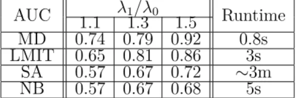
general model and specific applications for exact support recovery. Results for applications are presented and proved in the corresponding subsections in Sections 5.1 and 5.2. . . 95 6.1 AUC performance of various algorithms with different SNR values. . . 168
2·1 Channel coding communication framework. . . 7 2·2 Group testing example where {2,3} is the set of defective items. . . 10 2·3 Sparse linear regression example. . . 12 3·1 Plate model representation for the generative model considered in the
signal processing framework. . . 19 3·2 Channel model. . . 20 3·3 Sparse linear regression example and its mapping to the channel model. 21 4·1 Channel model representation of adaptive sparse recovery. . . 78 5·1 LBN vs. N for different SNR values, where LB is the necessity bound
given by (5.2) for K = 16, D= 512 and bmin =bmax= 1. For low levels
of SNR the necessary condition (N > LB, above the dotted line) is not satisfied even for very largeN, for fixed K andD. This is due to log1 +cSNRN behaving linearly instead of logarithmically for low SNRN ratios. . . 102 5·2 Illustration of SNR cutoff, K = 32, D= 512. . . 103 5·3 Mapping the multiple linear regression problem to a vector-valued
outcome and variable model. On the left is the representation for a single problem r = 1. On the right is the corresponding vector formulation, shown for sample indexn = 2. . . 116
Lasso. . . 119 5·5 Upper and lower bounds on the number of tests N. The logarithmic
dependence onDand linear dependence onK can be observed for large
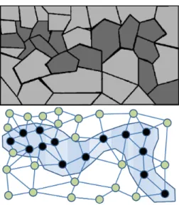
D. Also note that the bounds become tight asD→ ∞. . . 136 6·1 Illustration of a disease outbreak and its graph representation. Each
node corresponds to a county on the map and are connected to neigh-boring counties. The affected counties constitute a connected subgraph in the graph representation. The upper part of the figure is modified from (Patil and Taillie, 2003) and the lower part is taken from (Qian et al., 2014). . . 139 6·2 Disease outbreak detection in northeastern United States counties. . . 165 6·3 Performance of MD algorithm for different γ values. . . 167
CS . . . Compressive sensing
IID . . . Independent and identically distributed IT . . . Information theory
LHS . . . Left-hand side
LMI . . . Linear matrix inequality MD . . . Mirror descent
MI . . . Mutual information ML . . . Maximum likelihood
OMP . . . Orthogonal matching pursuit
PDF . . . Probability distribution/density function RHS . . . Right-hand side
RIP . . . Restricted isometry property SNR . . . Signal-to-noise ratio
SDP . . . Semidefinite programming
Chapter 1
Introduction
Recent advances in sensing and storage systems have led to the proliferation of high-dimensional data such as images, video or genomic data, which cannot be processed efficiently using conventional signal processing methods due to their dimensionality. However, high-dimensional data often exhibit an inherent low-dimensional structure, so they can often be represented “sparsely” in some basis or domain. The discovery of an underlying sparse structure is important to develop robust and efficient methods for all components of the signal processing pipeline, such as acquisition/sensing, storage, communication and analysis.
For instance in the case of signal acquisition, traditional approaches to sampling follow the guidelines set by the Nyquist-Shannon sampling theorem, where the sampling rate is taken to be twice the bandwidth of the underlying continuous signal. However, more recent approaches such as compressive sensing (CS) (Candès and Wakin, 2008) exploit the idea that the intrinsic “information rate” of a continuous signal can be may be much smaller than its bandwidth — in the case of CS this rate is related to the sparsity of natural signals when expressed in an appropriate basis.
In this dissertation we investigate the statistical and computational aspects of discovering the low-dimensional structure in high-dimensional data. In this context we consider two separate modalities that constitute the two parts of the manuscript. In the first part we investigate the theoretical limits of sparse recovery problems, where the aim is to discover the underlying sparse structure. We present a unifying
formulation which formally generalizes various sparse recovery problems. We then perform an information-theoretic analysis of the general model, inspired by the channel coding analysis in Shannon theory. This approach leads to tight lower and upper bounds on the statistical complexity in the form of intuitive mutual information formulas. We then evaluate these bounds for different problems and show that it leads to improved results for known problems or novel results for previously unexplored ones.
In the second part of the dissertation we consider the problem of connected subgraph detection in graph-structured signals, where the underlying low-dimensional structure to be discovered is characterized by constituting a connected subgraph of a given network. In contrast to the first part, we are mainly concerned with presenting a computationally efficient framework for formulating and solving the subgraph detection problem. To this end, we present a novel formulation and a corresponding optimization framework, and investigate its statistical and computational performance.
In Chapter 2, we introduce the necessary background by discussing the problems of channel coding, group testing and sparse linear regression related to the first part, and spectral graph theory related to the second part. Channel coding results and analysis are closely related to the results and analysis we will present in the proceeding chapter, while group testing and sparse linear regression are two important sparse recovery problems which we refer to often throughout the dissertation. In addition, previous results for group testing which we discuss serves as a starting point for our framework. We then discuss spectral graph theory as a tool for solving a multitude of problems over networks.
We present our main results for the first part in Chapter 3, starting with the formulation of the sparse recovery problem in a channel coding-like framework. We formally introduce the problem setup, then present information-theoretic lower and
upper bounds on the sample complexity for simple problems with discrete models, mostly following the prior results for group testing and then generalize this analysis to continuous models. We then extend our framework to problems with latent factors modifying the observation model, which allows the analysis of a very general class of sparse recovery problems. Surprisingly, we show that both upperand lower bounds are governed by the worst-case mutual information with respect to the latent factor, even though we consider an average-case error analysis. Consequently we show that the lower and upper bounds are tight, similar to the simpler setup considered before. We also extend the upper bound analysis to arbitrary models, whereas it was previously constrained to “non-scaling” models where certain problem parameters were independent of the asymptotically scaling factors. We prove that simple regularity conditions related to the continuity and smoothness of the distributions parametrizing the problem are sufficient for this extension. We conclude this chapter with comparisons to related work in the sparse recovery and information theory literature.
In Chapter 4, we consider two major extensions to the results in Chapter 3 and discuss possible connections to the problem of feature selection in statistical learning. We first investigate two different approaches to extend our analysis to problems with dependent covariates, in contrast to independent covariates in Chapter 3. We start with a typicality analysis for the set of covariate samples to obtain a new upper bound, then take a different approach with a conditionally IID assumption. While the former approach is applicable to a more general setup, the latter approach also presents a tight lower bound and leads to more intuitive and simple upper bound. As the second major extension to the analysis, we next investigate the adaptive recovery paradigm. We formalize the adaptive approach in our framework and derive a lower bound for this case that allows us to compare adaptive and nonadaptive methods on a high level. Lastly, we discuss possible connections of our framework to feature selection
and identify the hurdles that need to be overcome to adapt the framework to such problems. We specifically consider the problem of mutual information estimation from data in statistical learning settings and present our results that allow the use of the mutual information formulas for feature selection.
Chapter 5 presents the analysis and results that apply our framework to specific sparse recovery problems considered in the literature. This chapter serves to justify our unifying approach and demonstrate its usefulness as we show that our results lead to bounds that are competitive with problem-specific analyses in the literature. We are also able to investigate a broader class of setups for most problems, which our general approach can handle easier compared to conventional analysis methods. We divide the applications to two classes: problems with linear and nonlinear observations. The first class comprises of the problem of sparse linear regression or compressive sensing. We compute sample complexity bounds for the classical setup for this problem that matches the lower and upper bounds in the literature. Then we consider a variety of extensions to the classical setup, such as correlated sensing matrices, correlated or time-varying sparse coefficients, adaptive sensing and multivariate observations. We also compare our theoretical results with the performance of widely used practical recovery algorithms, demonstrating performance gaps. For nonlinear models, we first look at problems with missing or noisy data. We prove a lower bound for generic missing data problems and derive upper bounds that improve upon known results for sparse linear regression with missing or noisy data. We then consider a binary regression problem in 1-bit CS, proving upper bounds and nonadaptive and adaptive lower bounds. We conclude with the application of group testing, where we also improve upon the prior work that inspired our analysis and extend the results to more general setups including adaptive testing.
in network data in Chapter 6 where the aim is to discover a low-dimensional subgraph structure in graph-structured data. In contrast to the previous chapters, in this problem we are concerned with obtaining a practical relaxation of the underlying difficult problem and presenting efficient algorithms to solve it. We first discuss the integer problem and develop a convex relaxation of the subgraph detection problem that results in an semidefinite optimization formulation, with provable guarantees on the connectivity of the resulting solutions related to the internal conductance of the subgraph. We next propose an efficient iterative framework for optimizing the convex relaxation that scales well with large problem sizes, and show computational guarantees. We present experimental results on real networks that demonstrate the feasibility and performance of our framework.
We conclude the dissertation with a discussion on the presented analysis and results throughout all chapters in Chapter 7. We also discuss future work and possible extensions of the subgraph detection problem presented in Chapter 6.
Chapter 2
Background
In this chapter we introduce several problems that motivate this thesis and inspire our analysis. These problems include channel coding, group testing and sparse linear regression, also called compressive sensing. In addition, we review the information-theoretic analysis of group testing problems in (Atia and Saligrama, 2012). Both the channel coding problem and the analysis of group testing is closely related to the information-theoretic analysis of sparse problems that we will present in Chapter 3. We refer to the problem of sparse linear regression often in our information-theoretic analysis in Chapter 3 and will also present specific results later in Chapter 5. Finally, we also introduce the concept of spectral graph theory and typical applications as background for Chapter 6.
2.1
Channel coding
Channel coding refers to the problem of communicating a message across a possibly noisy and/or distorted communication channel to a receiver (Cover and Thomas, 1991). The noisy channel coding theorem, stated by Claude Shannon in “A Mathematical Theory of Communication,” (Shannon, 1948) describes the “capacity” of the channel, which is the maximum possible efficiency of transmission and error-correction methods versus levels of noise interference and data corruption. This result characterizes the number of channel uses necessary to transmit a message that contains a certain amount of information.
ω
X
(
ω
)
Y
Figure 2·1: Channel coding communication framework.
We shortly formalize the problem and present the noisy channel coding theorem, following the exposition of (Cover and Thomas, 1991). Letω∈ {1, . . . , D}be a message that is transmitted, where the amount of information it contains is characterized by the number of possible values D that it can take. The message is encoded by an encoder to X(ω), a sequence of length N, as shown in Figure 2·1. The encoded message is then transmitted across a discrete memoryless channel, which we define as the following.
Definition 2.1.1(Discrete Channel). A discrete channel consists of an input alphabet X, output alphabet Y and a probability transition matrix p(y|x) that defines the probability of observing output symbol y∈ Y given symbol x∈ X is sent. A discrete channel is memoryless if the probability distribution of the output depends only on the corresponding input, and conditionally independent of past inputs or outputs.
The decoder receives a random sequence Y ∼ p(y|x) and outputs an estimate of the message, ˆω, with the knowledge of Y and the set of encoded sequences for all messages, X. The decoder makes an error if ˆω 6= ω. We define the rate of the communication system as R = logND in bits per transmission. We call a rate
achievable if there exists a sequence of encoders X and decoders g(X,Y) such that the probability of decoding error for anyωtends to zero asN → ∞. (We will formalize error and achievability definitions later in Chapter 3.)
Theorem 2.1.1 (Noisy channel coding theorem). For a discrete memoryless channel, all rates R such that
R < C ,max
p(x) I(X;Y) (2.1)
is achievable, where I(X;Y) denotes the mutual information between random variables
R > C, there does not exist a sequence of encoders and decoders such that the probability of error tends to zero.
Note that we can also write (2.1) in the following way:
N >min
p(x)
logD
I(X;Y), (2.2)
which will be more convenient to compare with the later results we obtain.1
It is worthwhile to note that proofs for the achievability portion of the theorem typically consider random codebooks with codewordsX(ω) generated such thatX(ω1)
andX(ω2) are statistically independent for anyω1 6=ω2. Then either a joint typicality
decoder or a maximum likelihood decoder is considered and analyzed. While we note that we will utilize a similar maximum likelihood decoder in Chapter 3, we refer to (Cover and Thomas, 1991) for proofs of the theorem using joint typicality and (Gallager, 1968) for proofs using the maximum likelihood decoder.
2.2
Group testing
Group testing (Atia and Saligrama, 2012) is a form of sensing with Boolean arithmetic, where the goal is to identify a set of defective items among a larger set of items. As an example, group testing has been used for medical screening to identify a set of individuals who have a certain disease from a large population while reducing the total number of tests. The idea is to pool blood samples from subsets of people and to test them simultaneously rather than conducting a separate blood test for each individual. In an ideal setting, the result of a test is positive if and only if the subset contains a positive sample. A significant part of the existing research is focused on combinatorial pool design to guarantee detection using a small number of tests. Several variants of the problem exist, such as noisy group testing with different types of errors. An
interesting variant is the graph-constrained group testing problem, where the salient set is the set of defective links in a graph and each test is a random walk on the graph (Cheraghchi et al., 2010). The group testing model can be represented graphically as in Figure 2·2, where X is a Boolean testing matrix and Y is the outcome vector. Again, the different columns of the testing matrix correspond to the variables X, while the defective set corresponds to set S. Then, a test outcome Y only depends on XS,
which captures the presence or absence of defective items in the test.
The analysis of the complexity of the problem aims to characterize the number of tests N needed to reliably identify set S of K items among a total of D items, in terms of D, K and possibly other problem parameters such as noise level in case of noisy tests. The majority of the analysis is combinatorial in nature; it aims to determine testing strategies that allow the set to be identified deterministically by combinatorially designing the testing matrix (Du and Hwang, 2000). Adaptive versions of group testing have also been investigated by (Aldridge, 2012; Baldassini et al., 2013) where lower bounds are derived and adaptive algorithms are analyzed (see ref.s in (Baldassini et al., 2013)).
This problem was also formulated in a channel coding framework with random test constructions in (Atia and Saligrama, 2012) and in the past, in the Russian literature by (Malyutov and Mateev, 1980; Malyutov, 1976; Malyutov, 1978; Malyutov, 1979; Dyachkov, 2003). These work use channel coding-type analyses to determine information-theoretic limits on the number of tests N. We are particularly interested in the analysis of (Atia and Saligrama, 2012), as it forms the basis of our approach for analyzing the general class of sparse problems in an information-theoretic framework in Chapter 3.
We now present a short setup of the framework in (Atia and Saligrama, 2012) and present its main results. The defective set S is assumed to be chosen uniformly
N
D
Figure 2·2: Group testing example where {2,3}is the set of defective items.
at random from the collection of all sets of K items among D items. As in Figure 2·2, X denotes the N ×D testing matrix, which is a matrix with binary elements where each row represents the indicator vector for inclusions of items in a test and different rows are different tests. It is assumed that each element of the matrix is an IID Bernoulli random variable. Y is an N-length vector of binary test outcomes. For the noise-free case, the outcome of the testsY is deterministic. It is the Boolean sum of the codewords corresponding to the defective set S, given by Y =W
i∈SXi.
It is worthwhile to note that the model considered for Theorem 2.2.1 is non-scaling w.r.t. K and the distributions (i.e. K is fixed, D→ ∞and the distributions p(x) and
p(y|xS) are independent of D andN), whereas Theorem 2.2.2 is not constrained to
that case.
Below we present the two results derived for the group testing model which encapsulates noiseless and noisy variants, along with different probabilities p for
p(xk)∼Bernoulli(p).
Theorem 2.2.1 (Theorem III.1, (Atia and Saligrama, 2012)). Let (S1, S2) be any
partition of S to i and K−i variables respectively where i∈ {1, . . . , K} and >0 is a constant independent of K and D. Then, if the number of tests N is such that
N >(1 +) max
i=1,...,K
logD−Ki
I(XS1;XS2, Y|S)
then asymptotically the average error probability of recovering S approaches zero.
We remark that above theorem also considers the corrections to (Atia and Saligrama, 2012) in (Atia et al., 2015).
Theorem 2.2.2 (Theorem III.2, (Atia and Saligrama, 2012)). Let (S1, S2) be any partition of S to i and K −i variables respectively. Then, a necessary condition to recover S with an arbitrarily small average error probability is
N ≥ max
i=1,...,K
logD−Ki +i
I(XS1;Y|XS2, S)
. (2.4)
Using above results, specific bounds for noiseless and noisy variants of the group testing problem are derived in (Atia and Saligrama, 2012), which follow directly through the computation of mutual informationI(XS1;Y|XS2, S) for different values
of i. As an example, N = Ω(KlogD) is found as both a necessary and sufficient condition for recovery for noiseless group testing for p= 1
K.
The derivation of the sufficiency result follows through the analysis of a generic maximum likelihood decoder, which compares likelihoods p(y|xS, S) for different sets
S, while the necessary condition was derived using Fano’s inequality (Cover and Thomas, 1991). We will use similar methodology to derive the results in Chapter 3, while greatly extending and generalizing the approach of (Atia and Saligrama, 2012).
2.3
Sparse linear regression and compressive sensing
Sparse linear regression (Donoho, 2006) is the problem of reconstructing a sparse signal from underdetermined linear systems. It is assumed that the output vector Y can be obtained from a K-sparse vector β through some linear transformation with matrix X, i.e., in the noisy case with noise W,
X
β
W
N×1 N×D
D×1
N×1
Y
Figure 2·3: Sparse linear regression example.
Nonlinear versions of the regression problem are also investigated, where the channel model also includes a quantization of the output. The sparse linear regression model with an example is illustrated in Figure 2·3.
There exists a large body of research on both theoretical analysis and recovery algorithms for sparse linear regression. Much of the existing theoretical analysis focuses on limits of sparse recovery in linear models based on sensing matrices drawn from the IID Gaussian ensemble (Wainwright, 2009a; Fletcher et al., 2009; Aeron et al., 2010; Akcakaya and Tarokh, 2010; Wu and Verdú, 2012; Reeves and Gastpar, 2012). In addition, much of this related literature is focused on estimation, sometimes as a preliminary step towards support recovery. Furthermore, most of the earlier prior work relied heavily on the design of sampling matrices with special structures such as Gaussian ensembles and RIP matrices (Candès, 2008). More recent related work for linear models also consider arbitrary measurement matrices, some example of which are (Wang et al., 2010) that considers zero-mean, unit variance IID entries or sparse matrices with Gaussian elements on the non-zero elements and (Reeves and Gastpar, 2013) with arbitrary matrices for linear sparsity and approximate recovery,
both obtaining lower bounds. (Tulino et al., 2013) utilizes the replica method and the decoupling principle to study recovery limits for non-IID matrices with certain freeness conditions.
In terms of methodology, information-theoretic tools similar to the ones we use in Chapter 3 have been utilized, especially Fano’s inequality (Cover and Thomas, 1991) based lower bounds (Akcakaya and Tarokh, 2010; Aeron et al., 2010; Wainwright, 2009b; Tang and Nehorai, 2010; Reeves and Gastpar, 2013). The authors in (Tang and Nehorai, 2010) adopt a similar approach to derive sufficiency bounds for direct support recovery, albeit their analysis is focused on a hypothesis testing framework with fixed measurement matrices. (Jin et al., 2011) approaches the linear model in an IT framework similar to our work, formulating it as a problem of channel coding over the Gaussian multiple access channel. Consequently they consider Gaussian measurement matrices and consider the extensions to other variants such as different noise models or multiple measurements.
Many different recovery algorithms have also been proposed and analyzed for the sparse linear regression problem, which we will not go into details of. These algorithms include Lasso (Candès and Plan, 2009; Wainwright, 2009b), non-convex iterative variants of lasso such as iteratively reweighted lasso (Candès et al., 2008) or orthogonal matching pursuit (OMP) variants (Chen and Caramanis, 2013). We discuss related work on this problem in further detail in Section 3.9 in the next chapter.
We note that the sample complexity bounds obtained for the problem are dependent on many factors, such as the noise level in SNR, the scaling of K w.r.t. D, the nature of non-zero elements βS of β and the distributions of sensing matrix elementsX.
2.4
Spectral graph theory
Spectral graph theory considers the study of graphs by utilizing the eigen-decomposition of graph-related matrices, such as the adjacency matrix or Laplacian matrix. In this section we introduce these matrices that describe the properties of the graph, quantities such as the conductance of a graph and define graph-cuts along with classical results related to it.
In this work we only consider undirected graphs. We let G= (V, E, w) denote an undirected connected graph with n nodes, where V ={1, . . . , n} denotes the set of nodes and E ={(i, j) :i, j ∈V are connected} the set of all edges with |E|=m. If the graph is weighted, wij denotes the weight of an edge (i, j)∈E and is considered 1
otherwise. For i∈V, we writedi for the degree of vertex iin Gand let d be an upper
bound on all di. We let the symmetric n×n matrix A denote the incidence matrix of
the graph, where Aij = Aji = 1 if (i, j)∈ E and zero otherwise. D is the diagonal
matrix of degrees with Dii =di. Finally, we define the Laplacian of the graph with
L=D−A.
A cut (sometimes called a vertex cut) on a graph is indicated with a subset of nodes S⊂V, which partitions the graph to two setsS and V \S. For the purposes of this work, the size of a cut S is given by the volume measures of S and V \S, where we define Vol(S) =P
i∈Sdi. Note that Vol(V) = 2m. For unweighted graphs,
|E(S, V \S)| is the number of edges that connect nodes inS to nodes outside S. For weighted graphs,w(S, V \S) similarly denotes the total weight of all such edges, which reduces to |E(S, V \S)| in the unweighted case.
One important quantity of the graph, which also factors in our analysis is the
conductance of a graph, also called the Cheeger constant. The conductance measures the internal connectivity of a graph, e.g. whether there exists a “bottleneck” in the
graph. We start by defining the conductance of a cut S, which is given by
φG(S) =
w(S, V \S)
min (Vol(S),Vol(V \S)).
The conductance of a graph is then given by the lowest conductance among cuts containing at most half of the volume of the graph, i.e.,
φG = min
S⊂V:Vol(S)≤Vol(V)/2φG(S).
Conductance is a natural graph-partitioning objective because of its intimate connection with the behavior of random walks. It is also widely used in practice as it plays a central role in the design of algorithms for problems such as clustering (Ng et al., 2002), image segmentation (Shi and Malik, 2000) and community detection (Aksoylar et al., 2017).
Eigenvalues of the Laplacian matrix have a special significance in characterizing the connectivity and conductance of a graph. First, note that all eigenvaluesλ1 ≤. . .≤λn
of L are real and nonnegative since the matrix is symmetric and positive semidefinite. Second, zero is always an eigenvalue of L, i.e., λ1 = 0, since L1n = 0 where 1n is
the all-one vector. In addition, the multiplicity of the zero eigenvalue is equal to the number of connected components in the graph (Chung, 1997).
An important result in spectral graph theory relates the conductance of a graph with the spectrum of its Laplacian, known as the Cheeger’s inequality (Chung, 1997).
Theorem 2.4.1 (Cheeger’s inequality). Let λ2(L) denote the second smallest
eigen-value of the normalized Laplacian defined by L=D−12LD− 1 2. Then, λ2(L) 2 ≤φG ≤ q 2λ2(L).
While the problem of computing the conductance φG of a graph is NP-hard,
minimiz-ing cut usminimiz-ing the correspondminimiz-ing eigenvector. We refer the reader to (Vishnoi, 2012) for a good overview of the conductance minimization problem and approximation methods using the spectrum of the Laplacian.
Chapter 3
Information-Theoretic Analysis of Sparse
Recovery
In this chapter, we present an information-theoretic analysis of the sample complexity of sparse recovery problems in a unifying framework. We characterize this problem as a version of the noisy channel coding problem and establish mutual information formulas that provide sufficient and necessary conditions on the number of samples required to successfully recover the salient variables. These mutual information expressions unify conditions for both linear and nonlinear observations. We later compute sample complexity bounds for various problems in Chapter 5 based on the mutual information expressions in this chapter.
We first formulate the sparse recovery problems in signal processing and set decoding frameworks, using sparse linear regression as an example in Section 3.1. We then present a formal setup for the problem, defining variables and overarching assumptions we use throughout the chapter in Section 3.2. We present our analysis methods and lower and upper sample complexity bounds for simple problems in Section 3.3. In the following sections, we generalize this framework to various modalities, to make it suitable for the analysis of a large class of sparse recovery problems. We extend it to include models with continuous variables in Section 3.4. We then consider latent observation models and present lower bounds in Section 3.5, followed by upper bounds in Section 3.6. The analysis for generalizing these results to scaling models are presented in Section 3.7. We collect our remarks on the derived results in Section
3.8 and conclude with a discussion of the literature on information-theoretic analysis of sparse problems in Section 3.9.
The material in Section 3.3 is a review of some of the results in (Atia and Saligrama, 2012), along with the corrections in (Atia et al., 2015) contributed to by the author. Other sections, including 3.4, 3.5, 3.6 and 3.7 are novel contributions and presented in (Aksoylar et al., 2016), however certain parts have also appeared in (Aksoylar et al.,
2012), (Aksoylar et al., 2013a) and (Aksoylar et al., 2013b).
3.1
Sparse recovery as set decoding
Consider the sparse linear regression problem, as outlined in Section 2.3, for which we have the system (2.5),
Y =Xβ+W,
where β is the unknown D×1 sparse vector that we aim to estimate with support
S andK ×1 vector on the support βS,X is a known N ×D sensing matrix, W is
an N ×1 noise vector and Y is the N ×1 vector of observations. The system-level formulation for this problem usually considers β to be the unknown input quantity, X the known side input to the system, W as the noise in the system and Y as the output of the system, which follows from the above equation.
Let us approach the above framework from a different point-of-view, which we will refer to as the signal processing formulation. Abstractly, let the set of variables
S, which we call the salient set, be generated from a distribution over sets of size
K among D items. Also let a latent factor βS (if it exists) be generated from a
distributionp(βS),P(βS|S)1. Let a 1×DvectorX be generated from a distribution
Q(X) and a corresponding observationY generated using the conditional distribution
1In the general case,β
S can be random and unobserved in which case it is a latent factor, or it can
be fixed and known in which case we say a latent factor does not exist and it is simply incorporated into the deterministic observation modelP(Y|XS, S).
X XS Y
S βS
N
Figure 3·1: Plate model representation for the generative model con-sidered in the signal processing framework.
P(Y|X, βS, S) =P(Y|XS, βS, S) conditioned on X, βS and S. We have N such
inde-pendent sample pairs (X, Y) which constitute (X,Y). Given (X,Y) and knowledge of the observation modelP(Y|XS, βS, S), the problem is to estimate the set of relevant
variablesS. We illustrate this generative approach with the plate model in Figure 3·1. We can describe the formulation of sparse linear regression with the above frame-work as follows: S is the sparse support of β, each X corresponds to a rowX(n) of the sensing matrix and each Y corresponds to an element Y(n) of the observation
vector, forn = 1, . . . , N. The effect of noise is encapsulated in the observation model
P(Y|XS, S), along with the effects of βS, the values of β corresponding to the indices
in S. This framework focuses on the estimation of the support S, rather than the whole vector β.
It is important to note that this formulation is more general than the linear model that we considered above. Indeed, we observe that this formulation holds for the general class of sparse signal processing problems, including linear and nonlinear sparse regression problems, group testing, multivariate regression problems etc., with different X, Y and observation model definitions.
The fundamental observation we make about the formulation of sparse recovery problems in the above framework is the following: Among a set of D variables
X = (X1, . . . , XD), only K variables (indexed by set S) are directly relevant to the
β
SX
SY
S
Figure 3·2: Channel model. outcome Y is independent of the other variables {Xn}n6∈S, i.e.,
P(Y|X, S) =P(Y|XS, S). (3.1)
We also explicitly consider the existence of an independent latent random quantity affecting the observation model, which we denote with βS as above. Similar to (3.1),
with this latent factor we have the observation model
P(Y|X, βS, S) =P(Y|XS, βS, S). (3.2)
Note that the existence of such a latent factor does not violate (3.1).
In this chapter we will aim to analyze the sample complexity of this problem by establishing sufficient and necessary conditions on N to recover S with an arbitrarily small average error probability, in terms of the number of variables D, number of relevant variables K, observation modelP(Y|XS, S) and variable generation model
Q(X).
We perform the analysis of sample complexity by posing this identification problem as an equivalent channel coding problem (cf. Section 2.1), as illustrated in Figure 3·2. The salient setScorresponds to the message transmitted through a channel. The setS
is encoded byXS of lengthN, which is the collection of codewordsXn forn∈S, from
a codebookX. The coded messageXS is transmitted through a memoryless channel
P(Y|XS, βS, S) with output Y, with unknown side information/channel state βS. As
Y
X
β
β
SW
S
X
S N×1 N×D D×1 N×1{3, 5, 9}
Y
K×1Figure 3·3: Sparse linear regression example and its mapping to the channel model.
channel output Y and the codebook X. We call this framework “set decoding,” since we are transmitting a set-valued message through a channel and trying to decode it in the receiver. We illustrate the set decoding model for sparse linear regression in Figure 3·3.
The sufficiency and necessity results we present in this chapter are analogous to the channel coding theorem for memoryless channels, as presented in Theorem 2.1.1. These results are of the form
N >max ˜ S⊂S logD−||S\S|˜S|˜ IS˜ , (3.3)
where I˜S = ess infbI(XS\S˜;Y|XS˜, βS = b, S)2 is the worst-case (w.r.t. βS) mutual
information between the observation Y and the variables XS\S˜ that are in S but
not in ˜S, conditioned on variables in ˜S. For each subset ˜S of S, this bound can be
2The essential infimum of a measurable functionf is the greatest lower bound on the function
that holds everywhere except on a set of measure zero. Formally, for a measure space (X,Σ, µ), ess inff = sup{α∈R:µ({x∈ X :f(x)< α}= 0}.
interpreted as follows: The numerator is the number of bits required to represent all sets S of size K given that its subset ˜S is already known. In the denominator, the mutual information term represents the uncertainty reduction in the output Y
given the remaining input XS\S˜ conditioned on a known part of the input XS˜, in
bits per sample. This term essentially quantifies the “capacity” of the observation model P(Y|XS, βS, S). Then, the number of samples N should exceed this ratio of
total uncertainty to uncertainty reduction per sample for each subset ˜S to be able to recover S exactly.
3.2
Problem setup
Notation. We use upper case letters to denote random variables, vectors and
matrices, and we use lower case letters to denote realizations of scalars, vectors and matrices. Subscripts are used for column indexing and superscripts with parentheses are used for row indexing in vectors and matrices. Bold characters denote multiple samples jointly for both random variables and realizations and specifically denote N
samples unless otherwise specified. Subscripting with a set S implies the selection of columns with indices in S. Table 3.1 provides a reference and further details on the used notation. The transpose of a vector or matrix a is denoted by a>. log is used to denote the natural logarithm and entropic expressions are defined using the natural logarithm, however results can be converted other logarithmic bases w.l.o.g., such as base 2. The symbol ⊆ is used to denote subsets, while ⊂ is used to denote proper subsets.
Without loss of generality, we use notation for discrete variables and observations throughout the paper, i.e. sums over the possible realizations of random variables, entropy and mutual information definitions for discrete random variables etc. The notation is easily generalized to the continuous case by simply replacing the related
Table 3.1: Reference for notation used
Random quantities Realizations
Variables X1, . . . , XD x1, . . . , xD 1×D random vector X = (X1, . . . , XD) x= (x1, . . . , xD) 1×|S| random vector XS xS N×Drandom matrix X x n-th row of X X(n) x(n) d-th column of X Xd xd d-th elt. ofn-th row Xd(n) x(dn) N×|S| sub-matrix XS xS Observation Y y N×1 observation vector Y y n-th element of Y Y(n) y(n)
sums with appropriate integrals and (conditional) entropy expressions with (condi-tional) differential entropy, excepting sections that deal specifically with the extension from discrete to continuous variables, such as the proof of Lemma 3.3.1 in Section 3.4.
Variables. We letX = (X1, X2, . . . , XD)∈ XD denote a set of IID random variables
with a joint probability distribution Q(X). We specifically consider discrete spaces
X or finite-dimensional real coordinate spaces Rd in our results. To simplify the
expressions, we do not use subscript indexing on Qto denote the random variables since the distribution is determined solely by the number of variables indexed.
Candidate sets. We index the different sets of size K asSω with index ω, so that
Sω is a set of K indices corresponding to the ω-th set of variables. Since there are D
variables in total, there areDK such sets, therefore ω ∈ I ,n1,2, . . .DKo. We use
S without a subscript to denote the “true” set that we aim to estimate.
For any two setsSi andSj, we define Si,j,Si,jc, and Sic,j as the overlap set, the set
Namely, Si,j =Si∩Sj, Si,jc =Si∩Sjc=Si \Sj and Sic,j =Sic∩Sj =Sj \Si.
Latent observation parameters. In some of the following sections, we consider
an observation model which is not completely deterministic and known, but depends on a latent variable βS ∈ BK. We assume βS is independent of variables X and has a
prior distribution P(βS|S), which is independent of S and symmetric (permutation
invariant). We further assume that βk for k∈S has finite Rényi entropy of order 1/2,
i.e. H1
2(βk)<∞and also that H 1
2(βS) =O(K).
Observations. We let Y ∈ Y denote an observation or outcome, which depends only on a small subset of variablesS ⊂ {1, . . . , D}of known cardinality|S|=K where
K D. In particular, Y is conditionally independent of the variables given the subset of variables indexed by the index set S, as in (3.1), i.e., P(Y|X, S) = P(Y|XS, S),
where XS ={Xk}k∈S is the subset of variables indexed by the setS. The outcomes
depend onXS(andβSif it exists) and are generated according to the modelP(Y|XS, S)
(or P(Y|XS, βS, S)).
We further assume that the observation model is independent of the ordering of variables in S such that
P(Y|XS =xS, S) =P(Y|XS =xπ(S), S)
for any permutation mappingπ, which allows us to work with sets (that are unordered) rather than sequences of indices. Also, the observation model does not depend on S
except throughXS, i.e.,
P(Y|XSω =x, Sω) = P(Y|XSωˆ =x, Sωˆ)
for any x∈ XK,ω,ωˆ ∈ I.
condi-tional distribution given the true subset of variablesS. For instance, with this notation we have p(Y|XS) = P(Y|XS, S), p(Y|XS, βS) = P(Y|XS, βS, S), p(βS) = P(βS|S)
etc. When we would like to distinguish between the outcome distribution conditioned on different sets of variables, we usepω(· | ·) =P(· | ·, Sω) notation, to emphasize that
the conditional distribution is conditioned on the given variables, assuming the true setS is Sω.
We observe the realizations (x,y) of N variable-outcome pairs (X,Y) with each sample realization (x(n), y(n)) of (X(n), Y(n)),n = 1,2, . . . , N. The variables X(n) are
distributed IID across n = 1, . . . , N. However, if βS exists, the outcomes Y(n) are
independent for different n only when conditioned on βS. Our goal is to identify the
set S from the data samples and the associated outcomes (x,y), with an arbitrarily small average error probability.
Decoder and probability of error. We let ˆS(X,Y) denote an estimate of the setS, which is random due to the randomness in S, X and Y. We further let P(E) denote the average probability of error, averaged over all setsS of size K, realizations of variables X and outcomes Y, i.e.,
P(E) = Pr[ ˆS(X,Y)6=S] = X
ω∈I
P(ω) Pr[ ˆS(X,Y)6=Sω|Sω].
Scaling variables and asymptotics. We letD∈N,K ,K(D)∈Nbe a function of D such that 1≤K < D/2 and N ,N(K, D)∈N be a function of both K and D. Note that K can be a constant function in which case it does not depend on D. For asymptotic statements, we considerD → ∞and K and N scale as defined functions of D. We formally define sufficient and necessary conditions for recovery as below.
Definition 3.2.1. For a function g , g(N, K, D), we say an inequality g ≥ 1 (or
g > 1) is a sufficient condition for recovery if there exists a sequence of decoders
ˆ
g > 1) for sufficiently large D, i.e., for any > 0, there exists D such that for all
D > D, g ≥1 (or g >1) implies P(E)< . Conversely, we say an inequality g ≥1
(or g > 1) is a necessary condition for recovery if when the inequality is violated,
limD→∞P(E)>0 for any sequence of decoders.
In our asymptotic results, we will present bounds of the form LHS ≥RHS (or LHS
> RHS) which translate to the formal definition above usingg = LHSRHS.
Scaling and non-scaling models. We formally define scaling and non-scaling
models, which we distinguish between in our achievability analyses. Non-scaling models are models where the marginal variable distributionQ(Xk), latent variable distribution
P(βS|S) (if exists) and the observation modelP(Y|XS, βS, S) are independent of D
and N. We further restrict the analysis for these models to the case where K is independent of D, i.e., K(D) is a constant function. As a result, most “single-letter” quantities involving the problem, e.g. the single-letter mutual information
I(XS;Y|βS, S), do not scale with D and N, making the analysis easier in some cases.
Conditional entropic quantities. We occasionally use conditional entropy and
mutual information expressions conditioned on a fixed value or on a fixed set. For two random variables U ∈ U and V ∈ V, we use the notation H(U|V = v) =
−P
up(u|v) logp(u|v) to denote the conditional entropy of U conditioned on fixed
V =v. For a measurable subsetV0 ⊆ V of the space of realizations of V, H(U|V ∈
V0) = − 1
P(V0)
P
v∈V0p(v)Pup(u|v) logp(u|v) denotes the conditional entropy of U conditioned onV being restricted to setV0. Note that this is equivalent to the (average)
conditional entropy H(U|V) when V0 = V. The differential entropic definitions for
continuous variables follow by replacing sums with integrals, and conditional mutual information terms follow from the entropy definitions above.
To recap, we formally list the main assumptions that we require for the analysis in this chapter below.
(A1) Equiprobable support: Any set Sω ⊂ {1, . . . , D} withK elements is equally
likely a priori to be the salient set. We assume we have no prior knowledge of the salient set S among the DK possible sets.
(A2) Conditional independence and observation symmetry: The
observa-tion/outcome Y is conditionally independent of other variables given XS,
variables with indices in S, i.e., P(Y|X, S) = P(Y|XS, S). For any
per-mutation mapping π, P(Y|XS = xS, S) = P(Y|XS = xπ(S), S), i.e., the
observations are independent of the ordering of variables. We further as-sume the observation model does not depend on S except through XS, i.e.,
P(Y|XSω =x, Sω) = P(Y|XSωˆ =x, Sωˆ) for any x∈ X
K, ω,ωˆ ∈ I.
(A3) IID variables: The variables X1, . . . , XD are independent and identically
distributed.
(A4) IID samples: The variables X(n) are distributed IID across n= 1, . . . , N.
(A5) Memoryless observations: Each observationY(n) at samplen is independent of X(n0) conditioned on X(n).
3.3
Lower and upper bounds for discrete models
In this section we state a sufficient condition for the recovery of S, for the case of non-scaling models (i.e. K is fixed and Q(X), p(Y|XS) are independent of D and
N) and where X andY are discrete variables. We also assume there does not exist a latent variable βS that couples observations across samples n = 1, . . . , N. These
results follow in a straightforward manner from the analysis of (Atia and Saligrama, 2012) and we obtain the sufficiency bound presented in Theorem 2.2.1.
To derive the sufficiency bound for the required number of samples, we analyze the error probability of a maximum likelihood (ML) decoder (Gallager, 1968). For
this analysis, we assume that S1 is the true set Sω among ω ∈ I. We can assume
this w.l.o.g. due to the equiprobable support, IID variables and observation model symmetry assumptions (A1)–(A5), thus we can write
P(E) = N1 K X ω∈I Pr[ ˆS(X,Y)6=Sω|Sω] =P(E|S1).
For this reason, we omit the conditioning onS1 on the error probability expressions
throughout this section.
The ML decoder goes through all NK possible setsω ∈ I and chooses the set Sω∗ such that
pω∗(Y|XS
ω∗)> pω(Y|XSω), ∀ω 6=ω ∗
, (3.4)
and consequently, if any set other than the true set S1 is more likely, an error occurs.
This decoder is a minimum probability of error decoder for equiprobable sets, as we assumed in (A1).
We now state a simple upper bound on the error probability P(E) of the ML decoder, which is averaged over all sets, data realizations and observations. Define the error event Ei as the event of mistaking the true set for a set which differs from
the true set S1 in exactly i variables, thus we can write P(Ei) = Pr[∃ω6= 1 :pω(Y|XSω)≥p1(Y|XS1),
|S1c,ω|=|S1,ωc|=i, |S1|=|Sω|=K]. (3.5)
Using the union bound, the probability of error P(E) can then be upper bounded by P(E)≤ K X i=1 P(Ei) = K X i=1 X XS1 X Y Q(XS1)p1(Y|XS1)P(Ei|XS1,Y, ω= 1), (3.6)
conditioned on the true index ω= 1, the realization XS1 for the set S1, and on the
sequence Y.
We define the following quantity Eo(ρ) as the “error exponent” characterizing an
upper bound on the probability of error P(Ei).
Eo(ρ) =−log X Y X XS˜ X XS\S˜ Q(XS\S˜)p(Y, XS˜|XS\S˜) 1 1+ρ 1+ρ , 0≤ρ≤1, (3.7)
for any ˜S⊂S such that |S˜|=K −i. The following lemma provides an upper bound onP(Ei), using the error exponent definition.
Lemma 3.3.1. The probability of the error event Ei defined in (3.5) that a set selected
by the ML decoder differs from the set S1 in exactlyi variables is bounded from above
by P(Ei)≤e−(N Eo(ρ)−ρlog( D−K i )−log( K i)). (3.8)
The proof for Lemma 3.3.1 analyzes the upper bound in (3.6) and follows the proof of Lemma III.1 of (Atia and Saligrama, 2012), considering the corrections to the proof cited in (Atia et al., 2015). We reproduce the proof in Appendix A.1 for posterity, since we will refer to parts of it throughout the thesis.
We now restate Theorem 2.2.1 with the corrections made in (Atia et al., 2015), to emphasize the validity of the bound for discrete and non-scaling sparse recovery problems other than group testing. It follows from a Taylor series analysis of the error exponent, similar to the analysis of the ML decoder in (Gallager, 1968). Notice that we also change the notation from maximizing over i= 1, . . . , K and considering partitions (S1, S2) to an equivalent notation where we directly maximize over ˜S ⊂S
(which correspond to partitions (S\S,˜ S˜)).
of K and D. Then, if assumptions (A1)–(A5) are satisfied, N >(1 +)·max ˜ S⊂S logK−|D−KS|˜ I(XS\S˜;Y|XS˜, S) , (3.9)
is a sufficient condition3 for the average error probability to approach zero asymptoti-cally, i.e., limK→∞limD→∞P(E) = 0.
Note that it is sufficient to compute I(XS\S˜;Y|X˜S, S = ˆS) for one value of Sˆ (e.g. S1) instead of averaging over all possible S, since the conditional mutual information expressions are identical due to symmetry assumptions on the variable distribution and the observation model. Similarly, the bound need only be computed for one partitioning
(S\S,˜ S˜) for each |S˜| ∈ {0, . . . , K −1}, since the mutual information is identical for all such partitions.
While the above result applies to sparse recovery problems other than group testing, it is still very restrictive: We cannot analyze problems that contain continuous variables, have latent factors in the observation model, or scaling models – models where distributions either depend on N, D or where K also scales as a function of D. As an example, the sparse linear regression model in Section 2.3 contains continuous variables and possibly latent factorsβS in case the values of variables in the support
of β are random or not known.
To overcome these obstacles, in the following sections, we will modify the above analysis to a much larger class of problems by deriving major extensions to the analysis.
Finally, we note that the lower bound as derived in Theorem 2.2.2 also holds for discrete and continuous variables (which is considered in the next section) without latent observation variables, which we will consider later in Section 3.5. We also note that the proof in (Atia and Saligrama, 2012) has notational problems such as not conditioning on ˜S ⊂ S (S2 in the proof) and S
ω explicitly. Nevertheless the lower
bound we prove in Section 3.5 will be more general than Theorem 2.2.2 and will reduce
3“Sufficient condition” is defined formally in the problem setup, where in this case we have