Solving the Traveling Salesman Problem Using Ordered-Lists

(1)

Air Force Institute of Technology

AFIT Scholar

Theses and Dissertations Student Graduate Works

3-21-2019

Solving the Traveling Salesman Problem Using

Ordered-Lists

Petar D. Jackovich

Follow this and additional works at:https://scholar.afit.edu/etd

Part of theOther Mathematics Commons

This Thesis is brought to you for free and open access by the Student Graduate Works at AFIT Scholar. It has been accepted for inclusion in Theses and Dissertations by an authorized administrator of AFIT Scholar. For more information, please [email protected].

Recommended Citation

Jackovich, Petar D., "Solving the Traveling Salesman Problem Using Ordered-Lists" (2019).Theses and Dissertations. 2303.

(2)

Solving the Traveling Salesman Problem Using Ordered-Lists

THESIS

Petar D. Jackovich, 1st Lt, USAF AFIT-ENS-MS-19-M-127

DEPARTMENT OF THE AIR FORCE AIR UNIVERSITY

AIR FORCE INSTITUTE OF TECHNOLOGY

Wright-Patterson Air Force Base, Ohio

DISTRIBUTION STATEMENT A

(3)

The views expressed in this document are those of the author and do not reflect the official policy or position of the United States Air Force, the United States Department of Defense or the United States Government. This material is declared a work of the U.S. Government and is not subject to copyright protection in the United States.

(4)

AFIT-ENS-MS-19-M-127

SOLVING THE TRAVELING SALESMAN PROBLEM USING ORDERED LISTS

THESIS

Presented to the Faculty Department of Operational Sciences

Graduate School of Engineering and Management Air Force Institute of Technology

Air University

Air Education and Training Command in Partial Fulfillment of the Requirements for the Degree of Master of Science in Operations Research

Petar D. Jackovich, B.S. 1st Lt, USAF

21 March 2019

DISTRIBUTION STATEMENT A

(5)

SOLVING THE TRAVELING SALESMAN PROBLEM USING ORDERED LISTS THESIS

Petar D. Jackovich, B.S. 1st Lt, USAF

Committee Membership:

Lt Col Bruce A. Cox, PhD Chair

Dr. Raymond R. Hill, PhD Member

(6)

Abstract

The arc-greedy heuristic is a constructive heuristic utilized to build an initial, quality tour for the Traveling Salesman Problem (TSP). There are two known sub-tour elim-ination methodologies utilized to ensure the resulting tours are viable. This thesis introduces a third novel methodology, the Greedy Tracker (GT), and compares it to both known methodologies. Computational results are generated across multiple TSP instances. The results demonstrate the GT is the fastest method for instances below 400 nodes while Bentley’s Multi-Fragment maintains a computational advantage for larger instances.

A novel concept called Ordered-Lists is also introduced which enables TSP in-stances to be explored in a different space than the tour space and demonstrates some intriguing properties. While computationally more demanding than its tour space counterpart, the solution quality advantages, as well as a possibly higher pro-portion of optimal occurrences, when optimality is achievable via the ordered-list space, warrants further investigation of the space. Three meta-heuristics that lever-age the ordered-list space are introduced. Testing results indicate that while at a severe iteration disadvantage, these methodologies benefit from using the ordered-list space which yields a higher per iteration improvement rate.

(7)

Acknowledgements

First, I would like to thank my dog, Modi, for tolerating the long hours I spent not giving him attention while I was at school or in my home office working on this thesis. I would like to thank my parents for listening to my weekly ramblings and emotional vents about this thesis. I would like to thank Dr. Raymond Hill for convincing me to pursue this thesis topic. Finally, I’d like to thank my research advisor, Lt Col Bruce Cox, for putting up with my varying levels of motivation and excitement throughout the course of this thesis.

(8)

List of Figures

Figure Page 1. Konigsberg Bridges [1] . . . 3 2. Computational Complexity [2] . . . 6 3. TSP Relaxation Solution . . . 8 4. Cutting Plane [3] . . . 9

5. Greedy Worst Solution Example . . . 12

6. Greedy Subtour 1 . . . 20 7. Greedy Subtour 2 . . . 21 8. EL Subtour 1 . . . 22 9. EL Subtour 2 . . . 22 10. EL Subtour 3 . . . 24 11. MF Subtour 1 . . . 25 12. MF Subtour 2 . . . 26 13. MF Subtour 3 . . . 26 14. Greedy Tracker 1 . . . 29 15. Greedy Tracker 2 . . . 29 16. Greedy Tracker 3 . . . 29 17. Greedy Tracker 4 . . . 30 18. Greedy Tracker 5 . . . 30 19. Greedy Tracker 6 . . . 31 20. Greedy Tracker 7 . . . 31 21. GT Row Delete 1 . . . 33 22. GT modified 1 . . . 33

(11)

Figure Page

23. GT modified 2 . . . 34

24. GT modified 3 . . . 34

25. GT modified 4 . . . 34

26. Raw Data Snapshot . . . 37

27. Microbench Output . . . 38

28. Microbench Output Plot . . . 39

29. Proposed Future GT 1 . . . 42 30. Proposed Future GT 2 . . . 42 31. Proposed Future GT 3 . . . 43 32. Proposed Future GT 4 . . . 43 33. Ordered-Greedy 1 . . . 45 34. Ordered-Greedy 2 . . . 45 35. Ordered-Greedy 3 . . . 46 36. Perfect-Order 1 . . . 47 37. Perfect-Order 2 . . . 47 38. Perfect-Order 3 . . . 48 39. Perfect-Order 4 . . . 48 40. gr48 Optimal Tours . . . 49

(12)

List of Tables

Table Page

1. TSP Instances . . . 37

2. Greedy Sub-tour Methodology Run Times (Symmetric) . . . 40

3. Greedy Sub-tour Methodology Run Times (Asymmetric) . . . 41

4. 5 by 5 to 9 by 9 List vs. Tour Comparison . . . 50

5. Tour Distance Comparisons (Symmetric) . . . 52

6. Tour Distance Comparisons (Asymmetric) . . . 53

7. Greedy 2-Opt vs. PLGRS Comparison . . . 61

8. SA 2-Opt vs. PLGRS Comparison . . . 62

(13)

SOLVING THE TRAVELING SALESMAN PROBLEM USING ORDERED LISTS

I. Introduction

This thesis presents a novel sub-tour tracking and elimination methodology, the Greedy Tracker (GT), which ensures feasible solutions to the Traveling Salesman Problem during the implementation of the arc-greedy constructive heuristic. The GT is compared to other currently accepted sub-tour elimination methodologies to examine situational computational advantages. The paper then utilizes constructive heuristics to develop and explore a novel meta-heuristic that seeks to find an optimal, or near optimal, tour utilizing a novel concept called Ordered-Lists.

1.1 Motivation

Linear programming problems fall under the mathematical topic of optimization; they seek to optimize a linear function representing a measure of merit while minding linear equality and or inequality constraints on the systems performance [4]. The term linear programming was coined by economist and mathematician T.C. Koop-mans based on work that George B. Dantzig was doing as a mathematical advisor to the United States Air Force during the late 1940s. Dantzig later developed the “simplex method” to solve these linear programs which became widely accepted due to its ability to model important and complex management decision problems and its capability for producing solutions to many important linear programs in a reason-able amount of time. However, the simplex method was not reason-able to solve all LPs in a reasonable amount of time, leading mathematicians to seek an understanding on

(14)

mization problems are a subset of discrete linear programs that involve finding an optimal set from a finite set of solutions. While these problems theoretically have fewer possible solutions than a traditional linear program, they break the underlying continuity assumptions used in the simplex method thus preventing its usage. Other direct solution approaches to combinatorial optimization problems have also proved intractable, due to their exponential computational growth as problem size increases. One such combinatorial optimization problem that has long captured the interest of mathematicians is the traveling salesman problem.

1.2 The Traveling Salesman Problem

Applegate et al [5] describes the traveling salesman problem as, “Given a set of cites along with the cost of travel between each pair of them, the traveling salesman problem, or TSP for short, is the problem of finding the cheapest way of visiting all the cities and returning to the starting point.” It can also be mathematically defined as, given a complete undirected graph G = (V, E), cities are represented via the graph vertices, and edges represent the paths between the cities where the edge weights are the distances between each city. In terms of a graph the problem can be posed as: What is the shortest tour that visits all vertices once and returns to the starting vertex? One of the earliest examples of a similar graph problem was that of Euler’s bridge conundrum in Konigsberg. The city of Konigsberg consisted of four land areas separated by two branches of the river Pregel but connected by seven bridges. Euler analyzed the challenge of finding a way to cross all the bridges exactly once and return to the origin. This problem differs from the TSP as it seeks to travel each arc once, and return to the starting node. However, while different, Euler’s problem established much of the graph theory that is utilized to define problems like the TSP. The exact origins of the TSP are not known and there are many examples of

(15)

Figure 1. Konigsberg Bridges [1]

other similar early concepts. The first recorded use of the phrase “Traveling Salesman Problem” occurred in 1949 by Julia Robinson in her paperOn the Hamiltonian game

(a traveling salesman problem) [5]. When traditional linear programming methods

were applied to the TSP, intractability issues arose [5]. It has since been shown this is because the TSP falls into a class of known computationaly ‘hard’ problems called NP-Complete [6]. As a result, nontraditional methods such as heuristics are often used when solving the TSP.

A heuristic is a “method which, on the basis of experience or judgment, seems likely to yield a reasonable solution to the problem, but which cannot be guaranteed to produce the mathematically optimal solution” [7]. This is the key difference between a heuristic and an algorithm. An algorithm guarantees optimality, whereas a heuristic does not. Heuristics have many advantages over algorithms, especially when it comes to the class of NP-Complete problems. Evans and Zanakis [8] present a multitude of these reasons, but considering the intractability of the TSP, the primary reason is that while “An exact method is available. It it is computationally unattractive due to excessive time and or storage requirements. Large real-world complex problems

(16)

may prevent an optimizer from finding an optimal or even a feasible solution within a reasonable effort. Heuristics, on the other hand, can produce at least feasible solutions with minimal time and storage requirements.”

Many heuristics utilize a greedy-type methodology, where the best choice accord-ing to some predefined parameter is selected at each step of the method. An example of a greedy-type method for the TSP is the arc-greedy constructive heuristic, where the shortest available arc is added to the tour. However, this greedy heuristic runs the risk of generating sub-tours. These sub-tours are disconnected tours of less than size N (where N is the number of nodes present in the graph) that prevent a single continuous tour from being formed. Some research has been completed to develop methodologies that avoid sub-tours when utilizing the arc-greedy heuristic [9][10].

1.3 Research Questions

1. This paper introduces a novel sub-tour elimination methodology for the arc-greedy heuristic that is compared to two known sub-tour elimination method-ologies. Computational results are generated across multiple TSP instances for each method.

2. A novel concept called Ordered-Lists is introduced which enables TSP instances to be explored in a different space than the tour space. This concept demon-strates some intriguing properties which we leverage in some novel meta-heuristics.

1.4 Outline

In Chapter 2, various methods used to solve the TSP are reviewed. In Chap-ter 3, two known arc-greedy sub-tour tracking and elimination methodologies are introduced with pseudo code, examples, and theoretical advantages. This chapter also introduces a novel sub-tour elimination method, the Greedy Tracker. Chapter 4

(17)

summarizes each of these methodologies performance across different instances of the TSP focusing on run-time comparisons and identifying run time trends due to under-lying instance structure. In Chapter 5, a novel concept for viewing TSP instances, Ordered-Lists, is introduced and a novel TSP meta-heuristic utilizing this concept is proposed. In Chapter 6, results from the proposed meta-heuristic are summarized fol-lowed by Chapter 7 where, all results are concluded with recommendations on future research of utilizing the arc-greedy methodology on the TSP and other combinatorial optimization problems.

(18)

II. Literature Review

In this chapter several well known algorithms and heuristics used to solve the TSP are introduced. The chapter starts with a brief overview of NP-Hardness and is followed by the Linear Programming formulation of the TSP, an overview of heuristic methods, and an introduction to popular construction and meta-heuristic’s specif-ically used on the TSP. Understanding these motivates the sub-tour elimination methods for arc-greedy constructive heuristics as well as methodologies used in the Ordered-List meta-heuristics introduced later in this paper.

2.1 NP-Hardness

The TSP is an NP-Complete problem [6]. NP-complete is one of the classes of computational complexity. The other classes P, NP, and NP-hard along with their currently understood relationships are found in Figure 2. Briefly, the class P consists

Figure 2. Computational Complexity [2]

of problems solvable in polynomial time [2], the class NP consists of problems whose solutions can be verified in polynomial time. It is an open question if the class P is equivalent to class NP [11]. In additions, the class NP-hard can be informally thought of as the class of problems that are ”at least as hard as the hardest problems in NP.” The intersection of NP-Hard problems , and NP problems is called NP-complete. No

(19)

one has yet developed an efficient method for solving large instances of NP-complete problems to optimality [12]. The inclusion of the TSP in the set of NP-complete problems motivates the usage of other solving techniques such as LPs with cuts and heuristics.

2.2 LP Relaxation

The LP formulation for the the TSP as initially described by Dantzig et al [13] is given as:

minimize cTx

subject to 0≤xe ≤1 f or all edges e, X

(xe : v is an end of e) = 2 f or all cities v.

(1)

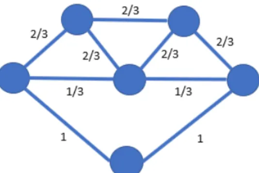
In this formulation, the decision variablexerepresents the choice of including edgeein the tour. The objective function associates a cost matrix with this decision variable, while the constraints ensure that each edge is used at most once and that each node has “two edges”. The authors, however, go on to discuss that this formulation is not the actual problem they want to solve, but is instead the problem they can solve. The formulation above is a relaxation of the actual problem which allows for a solution containing sub-tours, as well as solutions that partially assign edges. For instance, Figure 3 shows a allowable solution to (1), as it satisfies all constraints however it does not produce a single continuous tour. The answer found from the relaxation is however still useful as it provides a lower bound objective value for a TSP instance which can then be used to grade the quality of a proposed tour found by heuristics, or as a foundation for cutting plane algorithms.

(20)

Figure 3. TSP Relaxation Solution

2.3 Cutting Plane Method

Research from Heller [14] and Kuhn [15] indicated it may be possible to define beforehand a finite list of inequalities to add to the LP relaxation to exactly define the feasible region. However, the full list of inequalities could be far too large for any linear programming solver to handle directly. One methodology proposed by Applegate et al [5] to utilize this list is to implement a series of iterative cuts to remove infeasible solutions. A cut, or cutting plane, is a linear inequality that constricts the convex hull of the feasible region. The process of adding these cuts involves solving the LP relaxation, examining the solution to determine if it is a feasible tour, determining which additional inequalities are necessary to break any sub-tours, adding them and resolving the problem. This continues until a feasible, and thus optimal solution, to the TSP is found. Iterative cutting is possible because not every inequality needs to be added to the LP to find the optimal solution. Therefore, by solving multiple smaller LPs and iteratively adding cutting planes to remove infeasible intermediate tour solutions, an optimal solution can be found. However, the time to solve grows exponentially depending on the number of cuts that may be necessary. Because of this, a heuristic solution methodology appears to be the best way to quickly produce good, if not optimal tours [9].

(21)

Figure 4. Cutting Plane [3]

2.4 Heuristics

The difficulties encountered in applying cutting planes motivate the usage of heuristic methodologies to solve the TSP. The earliest recorded use of heuristics traces all the way back to ancient Greek mathematical literature. The name heuristic comes from the Greek verb ”heurskein” meaning ”to find”. From then to now people have been applying creative methodologies to solve difficult problems. As the name implies, some of the earliest examples of the TSP were records of various Salesman discussing the idea that more thought should be put into how they organize their journeys, or tours, to neighboring cities. A excerpt from the Commis-Boyageur, a 1830s German traveling salesman handbook [5], was brought to the attention of the TSP research community by Heiner Muller-Merbach in 1983 which translated to, ”The main thing to remember is always to visit as many localities as possible without having to touch them twice.” This excerpt indicates that as early as the 1800s, a salesman was cog-nizant that his routes should be planned as to minimize the number of places he visits more than once.

(22)

There are many desired qualities that make a good heuristic. Evans and Zanakis [8] give a list of characteristics they feel defines a good heuristic:

• Simplicity,

• Reasonable core storage requirements, • Speed,

• Accuracy, • Robustness,

• Acceptable to multiple starting points, • Produce multiple solutions,

• Good stopping criteria, • Statistical estimation, and • Interactive.

While many of these are intuitive, some may require further explanation. Because a heuristic does not necessarily converge to the optimal solution like a algorithm, the starting point, or initial solution, is very important. Different feasible initial solutions start at different locations within the feasible region and can often converge to dif-ferent local optima. By making a heuristic acceptable to multiple starting solutions, it has a better chance to test and explore more of the feasible region. As it’s Greek root implies, A heuristic also needs to have a good stopping mechanism to determine when it has ”found” a suitable solution. This ensures that the heuristic does not run for a unreasonably long time searching for answers without improvement. It also ensures the the heuristic does not stop before possibly reaching a very good set, or neighborhood, of new solutions.

Most heuristics can be broken into three categories, construction heuristics, local-search heuristics, and meta-heuristics. In relation to the TSP, construction heuristics

(23)

build a tour from scratch, local heuristics improve a given tour, and meta-heuristics apply a combination of constructive and iterative local-search heuristics [16], of partic-ular note is a meta heuristics ability to be interactive. Modern meta-heuristics often include user definable elements, which allow the user to tune the meta-heuristic for the given instance it is solving. These elements often include number of iterations, stopping criteria, number of initial starting solutions generated, and the definition of neighboring solutions, all of which are very important to how the meta-heuristic performs with regards to many of Evans and Zanakis’s qualities.

2.5 Greedy-type Construction Heuristics

One of the most common construction heuristic methodologies is the greedy heuris-tic. A greedy heuristic is one that at each step selects the best decision for a given metric, with no regard to how such choices may effect future decisions. For the TSP, there are three primary greedy construction heuristics; Nearest neighbor (node-greedy), arc-greedy, and Recursive Selection.

Nearest Neighbor (node-greedy heuristic).

The nearest neighbor(NN) heuristic was first applied to the TSP in a 1954 paper by Flood [17] but was introduced as the ”next closest city method.” The process was later refined by Dacey [18] and coined with its eventual name. The NN starts at an arbitrary city, and successively visits the closest unvisited city. It is important to to note that the nearest neighbor heuristic maintains a single path fragment that originates at the predetermined starting city, and cannot be closed into a cycle until every node has been visited. Therefore the decision of “which arc to add” is limited to only those arcs that leave the current end node of the fragment, this yields an algorithm run time of O(N2). Future work by Bentley [9] allowed this heuristic to

(24)

perform inO(N log N). This methodology allows NN to quickly create an initial tour which avoids sub tours. However, this approach is extremely sensitive to the choice of starting node, especially in larger instances. This sensitivity leads to a common practice of running NN for all cities as the starting node to provide the best solution, which is never more than ([log N] + 1)/2 times the length of the optimal tour[19]. The shortfall of this heuristic is that one can easily create examples that cause the heuristic to produce the worst possible solution. A simple example of a scenario where this occurs can be seen in Figure 5. If Node A is selected as the starting node, the

Figure 5. Greedy Worst Solution Example

heuristic is stuck in a situation where it constantly crosses it’s own path to connect to the nearest node thus producing the worst possible solution for the given instance. This is a characteristic downfall that is quite common in many greedy heuristics due to the short term framing of the greedy decisions being made.

Arc-greedy Heuristic.

The arc-greedy heuristic was first introduced by Papadimitiou and Steiglitz [20] as a modification of a process first seen in a 1968 paper by Steiglitz and Weiner [21]. The heuristic is a more complex greedy-type TSP heuristic where all edges of the graph are sorted from shortest to longest. Edges are then added to the tour starting with the shortest arc as long as the addition of this arc will not make it impossible to complete a tour. Specifically, this means avoiding adding edges that make early cycles, and also avoiding creation of vertices of degree three. This process,

(25)

as originally proposed, requiredO(N2 _log_N_{) time. However, Bentley was also able to}

speed up this process to O(N log N) [9] in a paper introducing his Multi-Fragment (MF) version. This yields a similar run time to NN while maintaining a similar worst case solution quality. Arc-greedy’s tour construction methodology causes the heuristic to only produce a single solution for each instance where NN can arrive at different solutions based on starting point. This is one of the shortcomings of arc-greedy when related to NN; the failure to generate variability in the output tour. On average though, the arc-greedy heuristic tends to outperform NN in tour quality on a instance to instance basis[9], however there are problem instances where the arc-greedy heuristic is significantly outperformed by NN as the scope of the arc-arc-greedy, considering all arcs at any instance, is inherently more greedy than NN, whose decision is bound to a single node. Thus, the arc-greedy heuristic can create situations where the final arcs needed to connect the various fragments into a single tour are of poor quality.

Recursive-Selection Heuristic.

Taking the arc-greedy shortcoming into account, Okano et al [16] introduced a new heuristic known as the Recursive-Selection Heuristic (RS). Rather than sorting all arcs by length, the RS sorts all points by order of the distance between each point and its nearest neighbor and iterates through the list adding points as long as they do not create a degree of three or early cycles. Once it has iterated through the list, if any points still have a degree of one or zero, it will resort the list with the closest available nearest neighbors and iterate through again. No runtime performance was given for the RS, but the RS+2-Opt meta heuristic designed by Okano steadily outperformed the MF+2-Opt through many of the instances tested in [16]. This RS heuristic motivates one of the central research questions of this paper “What is the

(26)

best way to order the greedy decisions made when solving the TSP?” It appears that modifying the decision framework can change how well a greedy heuristic performs.

2.6 Greedy-type Construction Heuristic Modifications

Minimizing the Variance of Distance Matrix Greedy.

A recent modification to the arc based greedy heuristic utilizes work from a 1970 paper by Held and Karp [22] to produce an arbitrary real vector,π, which transforms the distance matrix D to D0 by stretching and manipulating the distances between each node [10]. In general, the optimal tour of both distance matricies are the same. This allows for the possibility of finding a vectorπsuch that when the arc based greedy heuristic is implemented on D0 a better solution is produced versus when the same heuristic runs onD. Further research by Wang et al [10] showed that the performance of the arc based greedy heuristic was significantly negatively correlated to the variance of D0. This motivates the remainder of the paper, finding a vector π that minimizes the variance of the distance matrix D0, thus producing better greedy solutions. The authors identify the fact that minimizing the variance of the distance matrix mitigates a key disadvantage of the arc-based greedy heuristic; the disadvantage being that the last few edges added are often very inefficient due to the non-forward-thinking, greedy nature of the methodology.

Greedy with Regret.

A greedy heuristic with regret modifies a greedy heuristic so that it may recon-sider past decisions to possibly improve the final solution. Hassin and Keinan applied this methodology to the TSP utilizing the Cheapest Insertion Heuristic [23]. Adding regret allows the greedy heuristic to correct one of its biggest faults, selecting the best decision at the present moment with no regard to what happens to future moves.

(27)

Has-sin and Keinan create a deletion step which allows the heuristic to delete a previously added edge to the sub-tour if it is more expensive than the current decision.

2.7 Meta-Heuristics

This section discusses three meta-heuristics that can incorporate greedy type ele-ments into their solution methodologies. As discussed earlier, a meta-heuristic com-bines both constructive and, sometimes multiple, local-search heuristics with tunable elements to achieve near, if not optimal, solutions.

Simulated Annealing.

Simulated annealing (SA) is a local search type heuristic, modeled after the anneal-ing process that occurs in metal and glass makanneal-ing. The heuristic was first introduced in 1953 by Metropolis et al [24] as a numerical simulation. This heuristic was then applied to specific combinatorial optimization problems in 1983 by Kirkpatrick et al [24], and finally the TSP, two years later in a paper by Cerny [25]. Additional tunable elements and advantages were added to a later iteration by Eglese [26] who noted that the crux of SA was the ability to tune its temperature parameters to probabilistically accept worse solutions in order to avoid the heuristic getting stuck in a local minima. This is accomplished by a ‘temperature’ control parameter that assigns a probability to accepting a worse solution when considering any neighbor solution. Generally, SA starts with a warm temperature, corresponding to a high probability of accepting worse neighboring solutions, and cools over time. Reheating functions can be applied so that the heuristic can climb out of local minima. The biggest weakness of SA is the difficulty in tuning the heuristic to different instances, the proper stopping criteria, the proper set of neighbors, and the fact that ideal heating and cooling functions can change drastically from instance to instance.

(28)

Genetic Algorithm.

Genetic Algorithms (GA) are modeled after the evolutionary process. This idea was first conceived in 1950 by A.M. Turing [27]. He came up with the following list of connections which he believed could be incorporated into a computerized process modeling hereditary evolution.

• Structure of the child machine = hereditary material, • Changes of the child machine = mutation,

• Natural selection = judgment of the experimenter.

D. B. Fogel [28] first applied this methodology to the TSP in 1988. The GA follows a Darwinian ”Survival of the Fittest” type mentality by first generating a random initial population. A percentage of the population is then selected and evolved through mutation and/or reproduction. This continues until a set termination criterion is met and the newly created individuals are then evaluated against a fitness parameter. A new population is generated from individuals with a specified fitness level and the population is once again evolved. Generally, GAs perform very well due to their ability to explore many solutions simultaneously and identify quality schema utilizing a concept known as intrinsic parallelism. Reeves describes schema as a “subset of a space in which all the strings share a particular set of defined values [29]. In the case of the TSP, schema may be tours that have a certain number of common values in a row. For example, if we have a 10 node TSP, the group of tours that have a common connection of 3-4-5-6 would be a schema. If those connections are efficient and occur in many of the higher fitness population a GA identifies the string as a quality schema. Intrinsic parallelism is the idea that information on many schemata can be processed in parallel [30]. The difficulty of GAs in relation to the TSP is that special precautions have to be taken to ensure that mutations do not cause incomplete tours. Multiple

(29)

methodologies ensuring feasibility of solutions via mutation and combinations of tours are discussed by Merz and Freisleben [31].

2.8 Lin-Kernighan Algorithm

The Lin-Kernighan (LK) heuristic was published in 1972 [32]. Various iterative improvements have been made to the LK since its conception, some of the most recent advances can be found in a paper by Rego et al [6] documenting LK variants as well as state-of-the-art data structures which play a key role in many of the improvements. The core of this heuristic involves an adaptive k-opt swap methodology that allows for a variable number of swaps to occur at each iteration.

2-Opt.

An example of a k-opt swap, the 2-OPT routine incrementally considers pairs of arcs for a swap. In order to perform a thorough local search, the 2-OPT routine increments through each node along the tour and considers all possible arc pair swaps at that point. One methodology for performing such a swap is to replace the interme-diate tour between two nodes with its reverse order. If the swap is shown to reduce to total tour cost, the swap is saved (but not executed) and compared against all other swaps in the current iteration. At the end of the iteration if an improvement has been saved, the improved tour is executed and becomes the new tour, and the process starts over. Generally k-Opt methodologies need to have a good starting so-lution to be effective. One of the best starting soso-lutions for a 2-Opt is the arc-greedy heuristic [16]. Thus one popular methodology is the arc-greedy+2-Opt. Pseudocode for this process can be seen in Algorithm 1.

(30)

Algorithm 1Arc-Greedy+2-Opt Pseudocode

1: Initialize Variables

2: Generate arc-greedy tour

3: BestCost & SaveCost = arc-greedy tour cost

4: BestTour & SaveTour = arc-greedy tour

5: while Stop <1do 6: i = 0 7: while i <Size-1do 8: i = i + 1 9: j = i + 1 10: while j <Size do

11: TESTtour = replace tour between i and j with reverse

12: Calculate TESTtourCost

13: if TESTtourCost <BestCost then

14: BestTour = TESTtour 15: BestCost = TESTtourCost 16: end if 17: j = j + 1 18: end while 19: end while

20: if BestCost <SaveCost then 21: SaveTour = BestTour 22: SaveCost = BestCost 23: else 24: Stop = 1 25: end if 26: end while Concorde.

The Concorde is a heuristic LP-type solver designed by Applegate et al [5] that incorporates various separation routines into a primary cutting-plane loop. It orders the routines by rough estimates of their computational requirements. Utilizing a controller type program cuts from a routine are added to the LP relaxation and the problem is solved. If the LP bound for the entire round of cutting planes is above a threshold value, the round is broke off, column generation is applied, and the code returns to the start of the loop. If the total improvement is less than the threshold, additional cuts from the next separation routine are added and the problem is solved

(31)

again. This continues until a total improvement bound is less than a designated threshold.

(32)

III. Arc-Greedy Subtour Elimination Methodologies

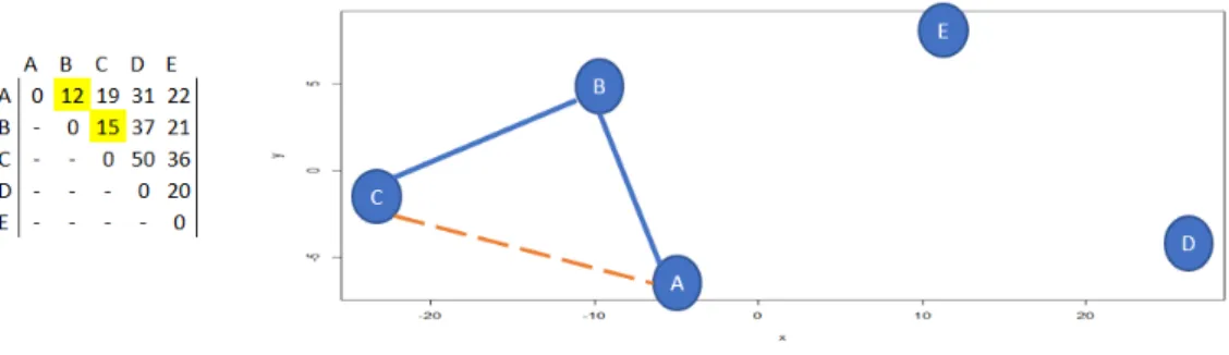
This chapter provides detailed explanations, examples, and pseudo-code for two known sub-tour elimination methodologies for the arc greedy TSP constructive tic as well as a third novel sub-tour elimination method. The arc based greedy heuris-tic gradually constructs a TSP tour by adding to the tour the shortest arc available at each iteration that does not cause a node to have a degree of more than 2 (see Figure 6). However, this degree constraint alone does not prevent sub-tours. The heuristic must also verify that a tour of less than size N, a premature partial circuit, called a sub-tour is not created. For example, consider the following tour construction utiliz-ing an arc greedy constructive heuristic methodology on a 5 node TSP instance. After

Figure 6. Greedy Subtour 1

adding the first two shortest arcs A-B and B-C, we can see from the distance matrix that arc A-C is the next shortest and still ensures that all nodes in the graph do not exceed a degree of 2. However, adding this arc creates a sub-tour, which would pre-vent the heuristic from ever constructing a feasible TSP tour (see Figure 7. There are two known methodologies for preventing sub-tours while using an arc greedy heuris-tic, namely Bentley’s Multi-fragment method [9], and an exhaustive loop test. This paper introduces a third novel method for eliminating sub-tours while using an arc greedy constructive heuristic. Each of the following methodologies were reproduced in R adhering strictly to the source descriptions and pseudocode.

(33)

Figure 7. Greedy Subtour 2

3.1 Exhaustive Loop

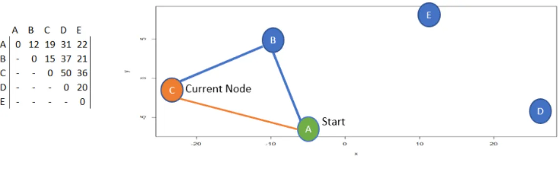
The Exhaustive Loop (EL), is a methodology for preventing sub-tours while using the arc greedy constructive heuristic. This method is not well documented in academic literature but is often simply referenced as “the standard way.” A literature review yielded no scholarly articles on this methodology. EL exhaustively cycles through every edge connected to the most recently added edge. Once a edge eij is added to the partial tour, node i will be identified as the “start node” and node j will be set as “current node.” A trace along the current partial tour then begins. At each step of the trace the “current node,” nodej, is checked to see if it is connected to another nodek via edgeejk in the partial tour. If it is, then node k becomes the new “current node.” If the trace returns back to the “start node” in under N steps. Where N is the number of nodes in the instance, then the added edge eij has created a sub-tour and is an illegal edge. If no edge leaves the “current node” the addition of edge eij is valid and the current portion of the tour is still a fragment. Each time a edge is added, a count is incremented and the process continues until N-1 edges have been added upon which the last two endpoints are then connected.

When applied to the earlier example, after adding edge A-C the heuristic identifies node A as the starting node and Node C as the current node (seen in Figure 8). The heuristic then looks at Node C and sees it has a degree of 2 and finds the other

(34)

Figure 8. EL Subtour 1

connected arc C-B. Node B becomes the current node and the heuristic verifies that the current node is not the same as the start node (seen in Figure 9). Once again, the

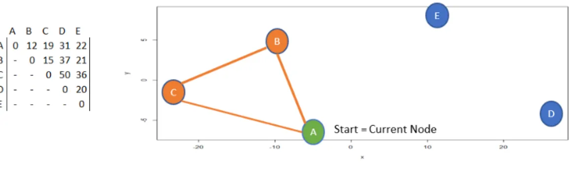
heuristic looks at the new current node, Node B, and identifies that it has a degree of 2 and finds the other connected arc B-A, and updates the current node to Node A. This time when the heuristic checks the current and start node, it realizes they are the same (Figure 10). It then sees how many edges have been added to the tour. Since the number is less than N, the heuristic marks that a subtour has formed and that arc C-A is not valid. Pseudocode for this methodology can be found in Algorithm 2.

Directional vs. Non-Directional.

The methodology above can be described as non-directional, where the direction of travel for each arc does not matter during tour construction. This methodology can only be used with symmetric TSP instances where the distance to travel from node to

(35)

Algorithm 2Exhaustive Loop Pseudocode

2: Sort edges: Shortest to Longest

3: while Nodes.Visited <Size-1 do

4: if Both nodes of current edge have degree <2 then 5: Set Start = Tail of current edge

6: Set Current = Head of current edge

7: while Continue = True do

8: if Current is Tail to Another Edge then 9: Set Next Node = Head of found edge

10: if Next Node = Start then

11: Subtour Formed — Remove Edge

12: Continue = False 13: else 14: Current = Next 15: end if 16: else 17: Continue = False

18: Set edge as part of tour

19: Nodes.Visited = Nodes.Visited + 1

20: end if

21: end while 22: end if

23: Next Edge in List

24: end while

(36)

node is equal in both directions. This poses some computational advantages as only

n∗(n+ 1)/2 arcs need to be initially sorted. The EL can also be modified to handle a directional methodology which can be used on both symmetric and asymmetric instances when the direction of the arcs is either of importance to the final solution and/or takes different distances to travel in each direction. In this directional scenario, all arcs of each direction n2₋_n_{, are sorted from shortest to longest and rather than}

tracking the total degree of each node, the connections are split into a T (To) and F (From) array. Utilizing these data structures ensures that each node is only entered once and left once ensuring a continuous direction throughout the tour.

3.2 Multi-Fragment

The Multi-Fragment heuristic described in Bentley’s [9] paper utilizes a unique non-directional methodology for eliminating subtours by focusing only on the ends (tails) of each tour fragment. The following structures are utilized in this methodol-ogy:

• An array, Degree, that keeps track of each nodes degree

• An array, Tail, that keeps track of the opposite tail of each fragment

All nodes are initialized as their own tail and given a degree of zero when the heuristic begins. As each arc is added, the tails of the nodes and fragment ends are updated.

(37)

While Bentley’s paper and pseudocode made no mention of how to update these tails, through testing, four possible scenarios were identified.

The first scenario is that the degree of both nodes of the added edge are 0, which is the same as 2 nodes being connected to form a new fragment. In this case, the heuristic sets the tail of each node equal to the node at the opposite end of the edge. Continuing with the 5 node example, this type of update occurs when the first edge is added. As seen in figure 11, when fragment A-B is added the tails for each node

Figure 11. MF Subtour 1

simply becomes the other node, and the degree of each is incremented. With respect to the graph, this scenario is just connecting two nodes.

The second and third scenario are fundamentally the same and occur when an added edge has one node with a degree of 1 and the other node has a degree of zero (for coding purposes they are separate scenarios dependent on which node node has a degree of 0 and which node has a degree of 0). With respect to the graph, this scenario is synonymous with a node being connected to a existing fragment. Figure 12 shows this scenario as node C is connected to the fragment made up of A and B. Node B’s degree is updated to be blank indicating that it is in the middle of a fragment. To update the other tail values, the heuristic must reference the tail B, which was A, and update it to show a tail of C, and then update the tail of C to what the tail of B previously was, or A.

(38)

connected by a new edge. See Figure 13, adding edge A-E utilizes a methodology

where the tail of each node that makes up the edge must have its tail’s tail updated to be the value of the opposite nodes tail. So in this case, node A’s tail, which was node C, must have its tail value updated to the tail value of node E, which is node D. The same updating must occur in respect to the other end of the fragment. Pseudocode for MF is included in Algorithm 3.

The description and pseudocode above depicts a non-directional methodology on a symmetric instance for constructing TSP tours using Benteley’s MF heuristic. It is possible to modify this methodology to function directionally on both symmetric and asymmetric instances. To do this, the degree array would be split into a To and From array as described when converting EL to a directional variant (see Section 3.1).

(39)

Algorithm 3Multi-Fragment Pseudocode

2: Sort edges(i,j): Shortest to Longest

4: if both nodes of current edge have degree ¡ 2 & Tail[i] is not j then 5: Add edge(i,j)

6: if Degree[i]=0 & Degree[j]=0 then 7: tempTaili = Tail[i]

8: tempTailj = Tail[j]

9: Tail[i] = tempTailj

10: Tail[j] = tempTaili

11: else if Degree[i]=1 & Degree[j]=0 then 12: tempTaili = Tail[i]

13: Tail[tempTaili] = Tail[j]

14: Tail[j] = tempTaili

15: Tail[i] = 0

16: else if Degree[i]=0 & Degree[j]=1 then 17: tempTailj = Tail[j]

18: Tail[tempTailj] = Tail[i]

19: Tail[i] = tempTailj

20: Tail[j] = 0

21: else if Degree[i]=1 & Degree[j]=1then 22: tempTaili = Tail[i] 23: tempTailj = Tail[j] 24: Tail[tempTaili] = tempTailj 25: Tail[tempTaili] = tempTailj 26: Tail[i] = 0 27: Tail[j] = 0 28: end if 29: Degree[i] = Degree[i] + 1 30: Degree[j] = Degree[j] + 1 31: Nodes.Visited = Nodes.Visited + 1 32: end if

34: end while

(40)

3.3 Greedy Tracker

The first original contribution this thesis makes is through the introduction of a novel way to track the progress of the arc greedy construction heuristic, and ensure sub-tours are not created. This new method is called the“greedy tracker” (GT). Con-ceptually, the GT serves as a methodology to track a nodes communication with other nodes when constructing a TSP tour. While GT can operate on both symmetric and asymmetric instances, it is conceptually easier to visualize the GT using its directional methodology on a symmetric instance and then generalizing the process for asymmet-ric instances or to the non-directional methodology on symmetasymmet-ric instances. Because of this, the following introduction to the GT utilizes the directional methodology on a symmetric matrix and is accomplished using the following structures:

• X = binaryn byn matrix of xij • F = binaryn by 1 array of fi • T = binaryn by 1 array ofti

• xij = 0 if arc from i toj is eligible, greater than 0 if not eligible • fi = binary for whether node i has been left

• ti = binary for whether node i has been entered

These structures track each move, and in doing so, prevent Hamilton cycles and sub tours. The process by which this is accomplished can be seen in Figure 14:

The X (identity), F (From), and T (To) structures can be seen above on the left and a distance matrix from the TSP can be seen on the right. The 1s loaded on the diagonal of the X matrix (where i=j) signal that these moves are ineligible. Note that the diagonal on the distance matrix has been colored red to correspondingly show these ineligible arcs. Looking at the distance matrix it can be seen that the shortest arc is either from A to B or vice versa, thus arc A to B is selected. The X,

(41)

Figure 14. Greedy Tracker 1

F, and T matrices are updated with 1s to indicate this move, this is shown in Figure 15.

Then, the column of the X matrix associated with the new arc is processed. Every row where a 1 appears is combined with the From row of the created arc. Figure 16 illustrates this operation. As seen in Figure 16, since Row 2 has a 1 in the same

(42)

as to not detract from their purpose of referring to an ineligible move, however in the code the values in each row will actually be added and values of greater than 1 will appear. For ease of reference in this example ineligible values in the distance matrix are turned red (Figure 17). As can be seen in Figure 17, distances that correspond

with a 1 in the X matrix have been made ineligible moves. Note that any row or column that has a 1 in the T or F arrays will also be marked as an ineligible move. This information will be utilized in the first step of the next iteration where the shortest available arc is identified. As seen in Figure 18, the shortest available arc is B-C and once again the X,F, and T matrices are updated with 1s to indicate the move. Once again the column of X associated with the “To” node of the new arc is

processed and every row where a 1 appears is combined with the “From” row of the created arc which can be seen in Figure 19. All the distances that correspond with a 1 in the X matrix are marked as ineligible moves in the distance matrix, as well as any distances associated with a 1 in the T and F arrays. The resulting step can

(43)

be seen in Figure 20. The red in the distance matrix indicates that adding arc A-C

is no longer possible because node C already has an edge entering it. This process thus removes the formation of the sub-tour shown earlier. The process shown above continues to iterate until all nodes have been visited which creates a Hamiltonian Path. The final connection to complete the tour is made using the T and F arrays as each should have one index that is still empty. Pseudo code for this methodology is in Algorithm 4.

This methodology can also be used on asymmetric instances as described, or may also be modified to handle a Non-Directional methodology for symmetric TSP instances. For this methodology, the T (To) and F (From) arrays are changed to a Degree array similar to the one used in MF. The row addition loop must also occur twice, once for every 1 in the column of the added edge (i, j), and once for every 1 in the column for the opposite edge (j, i). This nuance makes the GT quite inefficient

(44)

Algorithm 4Greedy Tracker Pseudocode

3: while Nodes.Visited <Size-1 do 4: if To[j]=0 & XMatrix[i,j]=0 then 5: Nodes.Visited + 1 6: XMatrix[i,j]=1 7: From[i]=1 8: To[j]=1 9: for k = 1 to size do 10: if XMatrix[k,j]=1 then 11: XMatrix[k,]=XMatrix[k,]+Xmatrix[i,] 12: end if 13: end for

15: end if 16: end while

17: Connect Hamilton Path

when utilized non-directionally as it doubles the computational time.

GT Improvements.

Certain adjustments to the GT methodology can be made to reduce the total number of operations that occurs within each iteration. These adjustments involve removing the addition of values in specific columns and rows as each node has been left and entered. This process decreases the dimensionality of the GT as the tour is constructed. This is possible because once a node has been entered, or left, no more arcs may enter that node or leave that node. Therefore, it is unnecessary to track what arcs could produce a sub-tour by entering or leaving that node. Consider the the same 5 by 5 instance used earlier, after completing row additions after adding arc A-B, column B can be deleted. Figure 21 shows the resulting GT and distance matrix. As can be seen, all moves in column B, or to Node B, are in eligible because Node B already has an arc entering it. Therefore, it is unnecessary to track and conduct row additions in this column. When working with a non-directional instance

(45)

Figure 21. GT Row Delete 1

a column would be deleted after the node had a degree of 2.

R struggles to re-dimensionalize matrices in an efficient fashion. Thus, modifi-cations to this methodology were made. Breaking down the process of the row and column delete methodology in greater detail yields the realization that only one nec-essary value, the tail of the current fragment, is being transferred to a new node. The GT is thus very similar to Bentley’s MF. When the diagonal is populated with 1s, the X matrix is initializing all nodes as their own tail and for the remainder of the tour construction the tail is passed as fragments are connected. In the case of the Directional GT only one value is passed because a directional fragment can only reattach to itself in one direction. This is why the non-directional GT requires two sweeps as opposed to the directional GT’s one. Consider the example below on the modified GT. Figure 22 shows a similar initialization to the original GT with the exception that the added arc is no longer reflected in the X matrix. After this step

(46)

empty, or 0 value in the “From” array. Figure 23 shows that this occurs in row B. The next step in the iteration is to find the value in row A that coincides with an

Figure 23. GT modified 2

empty value in the “To” array. Figure 24 shows that this value occurs at A. Thus

the next step is to set the intersection of the column identified in the previous step to the row identified directly before to a value of 1. In this case, the intersection of row B and column A is set to 1 as seen in Figure 25. In this first iteration the tail of A,

(47)

This process continues until a Hamiltonian path is formed. The pseudocode for this modified GT is in Algorithm 5.

Algorithm 5Greedy Tracker modified Pseudocode

3: while Nodes.Visited <Size-1 do 4: if To[j]=0 & XMatrix[i,j]=0 then 5: Nodes.Visited + 1 6: XMatrix[i,j]=1 7: From[i]=1 8: To[j]=1 9: Row = Intersect(which(X[,j]==0,which(From==0)) 10: Column = Intersect(which(X[,j]==0,which(From==0)) 11: XMatrix[Row,Column]=1

13: end if 14: end while

(48)

IV. Greedy Sub-tour Elimination Results

This section covers the TSP instances used, and testing methods employed, along with results from all three of the sub-tour elimination methodologies demonstrated in the prior chapter.

4.1 TSP Instances

TSP data for multiple instances and variations is available in an online library, TSPLIB, maintained by Ruprecht-Karls-Universitat Heidelberg located in Baden-Wurttemberg, Germany. The data from TSPLIP is available via one of two formats in an .atsp file type. A picture of the data’s raw format for these files can be seen in Figure 26. The first file type consists of a distance matrix containing a string of distances from node to node for all edges in the instance. However, the file is not properly formatted to be imported into R. To make this file type usable, the information was saved as a text string and then processed to place the information in matrix form. The second file type contains a series of coordinates for each node which can be utilized to form a distance matrix. The distances for every edge can be calculated via a euclidean distance formula (Equation 2) and placed into a distance matrix in R.

Euclidean Distance =p(x1−x2)2+ (y1−y2)2 (2)

The values also must be rounded. TSPLIB provides the best known optimal tours and scores for heuristic testing. For the purposes of this research testing was performed on the instances seen in Table 1, where the alpha prefix is an identifier and the numerical suffix indicates the instance size (in number of nodes).

(49)

Figure 26. Raw Data Snapshot

(50)

4.2 Testing

Initial tests verify that each sub-tour method (MF, EL, GT, Modified GT) pro-duced the same tour and distance for all TSP instances. These tests were conducted with both directional and non-directional versions of codes on symmetric TSP in-stances. In addition, the directional code versions were run on asymmetric TSP instances. Directional and non-directional codes were tested on symmetric TSP in-stances as they generally produce different solutions, and have different run times due to the number of arcs that must be considered.

Once testing verified each method produced identical greedy tours; that is all direc-tional code variants produced identical tours, and all non-direcdirec-tional codes produced identical tours, the remaining testing focused on computational run-time compar-isons. Each methodology was placed in the same arc-greedy heuristic shell so that testing would fairly compare the speed of the three sub-tour tracking and elimination methodologies. Bentley [9] and Wang [10] each utilized advanced computer tech-niques (k-d trees) and additional data structures to speed up the process of finding the next shortest arc available. However, since neither of these effect the speed of the sub-tour tracking and elimination methodologies they were not utilized.

Speed tests were conducted utilizing the R package “microbenchmark.” This pack-age allows testing of multiple R codes simultaneously. Microbenchmark randomly generates run order to handle possible CPU speed fluctuation during testing. The package also reports a variety of statistics to summarize run results. A sample of this output is in Figure 27. Microbenchmark output the minimum, mean, median,

(51)

and maximum run-times as well as the lower and upper quartiles. 100 iterations of each code were run to create these summary statistics on 13 different symmetric TSP instances and 9 asymmetric instances. Density plots of runtimes were also reported utilizing the Microbenchmark and ggplot2 R packages, an example of which are in Figure 28. Both symmetric and asymmetric instances were tested to determine if

Figure 28. Microbench Output Plot

symmetry effected run time.

4.3 Symmetric Instance Results

Mean run times for a variety of symmetric TSP instances utilizing each of the methodologies can be seen in Table 2. When looking at the directional methodolo-gies, the GT and modified GT tend to be the fastest methodologies on small instances followed by EL and MF. Once instance size reaches around 442, MF takes over as the fastest method for eliminating sub-tours. This largely is due to it’s linear growth in operation count as instance size grows. For larger instances, the heuristic is conduct-ing the same number of operations at each step. While the operations are slower for

(52)

Table 2. Greedy Sub-tour Methodology Run Times (Symmetric)

We see that the modified GT and original GT tend to perform very similar for smaller instances but once the instance size grows the elimination of the row addition opera-tions in the modified methodology gives the modified GT a computational advantage. The reduction in operations is still not enough to keep GT faster than MF as the searching procure utilized by the modified GT is still a computationally demanding process as instance size grows.

These performance trends are continued when looking at the non-directional code variants applied to these same symmetric instances as seen on the right half of Figure 2, with the exception of the original GT. In the non-directional instance, the dual row sweeping doubles the operations at each step, which gives the modified GT and EL a speed advantage. However, once again MF becomes the fastest methodology from the 442 node instance and larger.

4.4 Asymmetric Instance Results

The directional variants of each sub-tour elimination codes were also run on Asym-metric TSP instances to compare runtimes to determine if any trends changed. The mean runtimes are in Table 3.

There was greater variability between methods for some of the asymmetrical in-stances. This could be due to the how the edges fluctuate in each direction which

(53)

Table 3. Greedy Sub-tour Methodology Run Times (Asymmetric)

causes more searching to find edges to complete the tour. Prior overall trends remain, where modified GT is competitive for small to medium sized asymmetric instances, but MF is fastest for larger instances.

4.5 Future Improvements

The portion of the Modified GT most susceptible to computational growth is the search to identify what tail is necessary to move. If this search process growth can be limited, it is possible that the modified GT could outperform MF for larger instances as well. Some possible methodologies to limit computational growth include a better implementation of the row and column delete methodology in conjunction with a new row and column generation methodology. Size of the search operations could also be reduced drastically especially during the early iterations of the arc-greedy heuristic by only generating nodes and tails as needed. This is accomplished by storing a list of indices, call them Tnodes and Fnodes, for what arcs values are necessary for tail storage and transfer. The following example explains this methodology using the modified GT.

This proposed methodology starts with an empty X matrix. The To and From arrays are populated as usual, but the values searched when a tail is being moved, is limited to the indices contained within the subsets Tnodes and Fnodes. Therefore, for visual purposes, only nodes within these indicies show their values in the figures,

(54)

Figure 29. Proposed Future GT 1

represented as To[Tnodes] and From[Fnodes]. As with previous examples the first arc added is arc A-B. Figure 30 shows A and B are added to Tnodes and Fnodes, which generates a respective row and column for each to track the tail generated by the addition of the arc. This generation technique is possible because all unconnected

nodes initialize as their own tail. Utilizing the Modified Greedy Methodology any 1s in the ”To” column of the added arc that correspond with a 0 in the ”From” array will identify what row the tail will be transferred to. This is followed by searching the Row associated with the ”From” node of the current arc and identifying any nodes in this row that correspond with a 0 in the To array. This step can be seen in Figure 31. Once this step is completed, both rows and columns that correspond 1s in the “From” or “To” are deleted from the matrix and removed from the subsets Tnodes

or Fnodes(as seen in Figure 32). This process could drastically decrease the size of each iterations search larger TSP instances. This methodology along with coding in a more advanced computer language could help GT to maintain is performance gap over MF in larger instances.

(55)

(56)

V. Ordered-Lists Methodology

This section introduces a novel constructive heuristic called Ordered-Greedy. This is followed by a comparison of tour quality between the ordered-greedy output result-ing from 1000 random generated lists, versus viewresult-ing the lists as tours. This com-parison is performed for 13 symmetric instances, the outcome of which motivates the development of a new meta-heuristic based on Ordered-Lists.

5.1 Ordered-Greedy Heuristic

Given the sub-tour tracking abilities of the aforementioned methodologies, there are some interesting alterations to the arc-greedy heuristic that can be made. One such change is to utilize one of the elements realized by the Recursive Selection heuris-tic, where the order in which greedy decisions are made is taken into consideration. This concept motivated the development of a novel constructive heuristic called the Ordered-Greedy (OG) heuristic. The OG heuristic is a node-greedy heuristic that takes as input a complete list of nodes. Starting at the top of the list, each node is considered in turn and the available set of choices is limited to the feasible arcs originating at that node. What differentiates the OG from NN, another node-greedy heuristic, is that multiple fragments may exist during the tour construction.

The motivation for this heuristic is to apply a more structured approach to what nodes should be given priority in connecting to their nearest neighbors. Nodes higher in the list have maximum flexibility with minimal concern for node degree or sub-tours and thus typically choose better arcs than nodes later in the list. The quality of the solution found is heavily dependent on the order of the list.

To introduce the methodology of the OG heuristic, consider the following example. In this example an ordered list of D,E,C,B,A has been, through some unspecified

(57)

fashion, predetermined. This ordering of the nodes list is reflected in the matrix on the right-side of Figure 33 whose rows are now sorted according to this list order. The constructive heuristic now makes greedy decisions starting at the top of this list and working down. The first greedy decision is made with respect to node D. The

Figure 33. Ordered-Greedy 1

greediest, or shortest arc, from node D is arc D-E as indicated above. This arc and its associated node is tracked by the GT so that the next decision can be made. The next decision is made with respect to node E. This is not due to node E being the head of the previous arc added, but rather because it is second in the provided ordered list: D,E,C,B,A. Looking at the row in the Distance matrix associated with node E along with the GT output that captures ineligible moves (as seen in Figure 34), it can be seen that the shortest legal arc available is arc E-B. This process continues row by

row until the final row is reached which is where the T and F arrays are scanned to find the final legal arc as seen in Figure 35. After adding arc A-D, the resulting tour becomes A-D-E-B-C-A which is also the optimal tour for this TSP instance. This

(58)

result motivated the creation of the concept of a Perfect-Ordered List. Pseudocode for the OG is in Algorithm 6.

Algorithm 6Ordered-Greedy Pseudocode

2: Generate Order

3: Nodes.Visited = 0

5: Moves = arcs leaving Order[Nodes.Visited+1]

6: Moves[To==True]= Inf

7: Moves[XMatrix[Order[Nodes.Visited+1],]]= Inf

8: minmove = min(Moves)

9: Get First index i of Moves where Moves[i]=minmove

10: Add Arc(Order[Nodes.vistied+1],i) to tour

11: Track moves with Greedy Tracker 12: Nodes.Visited = Nodes.Visited+1

13: end while

14: Connect Hamilton Path

The OG non-directional and OG directional methodologies yield the same solu-tions because of how the OG handles connecsolu-tions to nodes that already have a degree of one. If a node attempts to connect to another node with a degree of 1, the con-nection will only be accepted if that node has already occurred in the order. This is because if the node has not yet occurred in the order, and the connection is allowed, the node will have a degree of 2 before its turn in the ordered-list. Thus, when its turn does come, it would not be able to make a connection. This behavior causes the non-directional to treat these nodes as if they were of the opposite direction, causing

(59)

the two methodologies to produce the same solution.

5.2 Perfect-Ordered List

A perfect ordered list (POL) is simply an ordered-list which, when iterated through using the ordered greedy heuristic described above, will yield the optimal solution. Most, but not all, optimal solutions can be associated with a POL (the reasoning for which is discussed later). To find whether a POL exists for a given optimal solution, following methodology based on the GT is used.

First, initialize by identifying all arcs in the optimal solution, and the shortest available Arc (using lowest index to break ties) for each node. Figure 36 shows the completion of this initialization. The next step is to then identify all, so called, Tier 1

Figure 36. Perfect-Order 1

nodes. These are nodes where the optimal arc is the same as the shortest arc available. During this iteration (seen in Figure 37), the only arc in the optimal solution that matches its shortest arc is Arc D-E.

(60)

This move is updated in the GT and the distance matrix is reanalyzed to determine the remaining shortest legal arc available for each node. The second iteration identifies any nodes that now match their shortest available arc with the optimal solution arc. These nodes are labeled as Tier 2 node. The intuition is that Tier 2 nodes derive their optimal arc matches as a result of the greedy decisions made by the Tier 1 nodes. As seen in Figure 38, the Tier 1 move effected the shortest available legal move for node E and is marked as a Tier 2 node. This process continues until either all nodes are

given a Tier as seen in Figure 39 or no greediest legal arcs match their optimal arc in an iteration. If the later occurs then no POL exists for the given optimal tour. If the

process does run to completion, then the order of the nodes are sorted with respect to their Tier. In the case of the example provided, the POL would be D,E,C followed by either A,B or B,A.

Order within the tiers does not effect the resulting tour, which reveals an inter-esting insight into solving the TSP using ordered-lists. More than one ordered list

(61)

corresponds to a single tour. Since the total number of permutations of nodes is equal for tours and ordered lists, we can deduce that certain feasible tours cannot be reached via the ordered list solution space. This information is cause for concern as it leads one to question whether the optimal tour is always achievable within the ordered list solution space. Tests on the 13 symmetric instances initially yielded POs for only 8 of the instances. However further testing on the GR48 instance revealed there exists multiple optimal tours. The images in Figure 40 show the difference between two unique optimal tours, one of which (left) cannot be represented by a Ordered List (i.e. cannot be found utilizing the OG Heuristic) and the other (right) can be found by the OG. Similar situations may exist for the larger instances but it

Figure 40. gr48 Optimal Tours

is nontrivial to find additional optimal tours for these large instances to verify. This line of inquiry is left as a question for future research.

5.3 Ordered-Lists vs. Tour Order

Since not all valid tours for an instance have an analog in the Ordered-List solution space, it is important to compare solution quality of each space. Exhaustive testing comparing all tour permutations and all ordered list permutations could only be completed on examples smaller than 10x10. Some 5x5 test instances were generated