Euler’s Method for Solving Initial Value Problems in Ordinary
Differential Equations.
Sunday Fadugba, M.Sc.
1*; Bosede Ogunrinde, Ph.D.
2; and Tayo Okunlola, M.Sc.
31
Department of Mathematical and Physical Sciences, Afe Babalola University, Ado Ekiti, Nigeria. 2
Department of Mathematical Sciences, Ekiti State University, Ado Ekiti, Nigeria. 3
Department of Mathematical and Physical Sciences, Afe Babalola University, Ado Ekiti, Nigieria.
E-mail: [email protected]*
ABSTRACT
This work presents Euler’s method for solving initial value problems in ordinary differential equations. This method is presented from the point of view of Taylor’s algorithm which considerably simplifies the rigorous analysis. We discuss the stability and convergence of the method under consideration and the result obtained is compared to the exact solution. The error incurred is undertaken to determine the accuracy and consistency of Euler’s method.
(Keywords: differential equation, Euler’s method, error, convergence, stability)
INTRODUCTION
Differential equations can describe nearly all systems undergone change. They are ubiquitous in science and engineering as well as economics, social science, biology, business, etc. Many mathematicians have studied the nature of these equations and many complicated systems can be described quite precisely with compact mathematical expressions. However, many systems involving differential equations are so complex or the systems that they describe are so large that a purely analytical solution to the equation is not tractable.
It is in these complex systems where computer simulations and numerical approximations are useful. The techniques for solving differential equations based on numerical approximations were developed before programmable computers existed. The problem of solving ordinary differential equations is classified into two namely initial value problems and boundary value problems, depending on the conditions at the end points of the domain are specified. All the
conditions of initial value problem are specified at the initial point. There are numerous methods that produce numerical approximations to solution of initial value problem in ordinary differential equation such as Euler’s method which was the oldest and simplest such method originated by Leonhard Euler in 1768, Improved Euler method, Runge Kutta methods described by Carl Runge and Martin Kutta in 1895 and 1905, respectively. There are many excellent and exhaustive texts on this subject that may be consulted, such as Boyce and DiPrima (2001), Erwin (2003), Stephen (1983), Collatz (1960), and Gilat (2004) just to mention few. In this work we present the practical use and the convergence of Euler method for solving initial value problem in ordinary differential equation.
NUMERICAL METHOD
The numerical method forms an important part of solving initial value problem in ordinary differential equation, most especially in cases where there is no closed form analytic formula or difficult to obtain exact solution. Next, we shall present Euler’s method for solving initial value problems in ordinary differential equations.
Euler’s Method
Euler’s method is also called tangent line method and is the simplest numerical method for solving initial value problem in ordinary differential equation, particularly suitable for quick programming which was originated by Leonhard Euler in 1768. This method subdivided into three namely:
Forward Euler’s method. Improved Euler’s method. Backward Euler’s method.
In this work we shall only consider forward Euler’s method.
Derivation of Euler’s Method
We present below the derivation of Euler’s method for generating, numerically, approximate solutions to the initial value problem:
))
(
,
(
x
y
x
f
y
(1) 0 0)
(
x
y
y
(2) Wherex
0andy
0are initial values forx
andy
, respectively. Our aim is to determine (approximately) the unknown function)
(
x
y
forx
x
0. We are told explicitly the value ofy
(
x
0)
, namelyy
0, using the given differential equation (1), we can also determine exactly the instantaneous rate of change ofy
at pointx
0))
(
,
(
)
(
x
0f
x
0y
x
0y
=f
(
x
0,
y
0)
(3) If the rate of change ofy
(
x
)
were to remain)
,
(
x
0y
0f
for all pointx
, theny
(
x
)
would exactlyy
0
f
(
x
0,
y
0)(
x
x
0)
. The rate ofchange of
y
(
x
)
does not remainf
(
x
0,
y
0)
for allx
, but it is reasonable to expect that it remains close tof
(
x
0,
y
0)
forx
close tox
0. If this is the case, then the value ofy
(
x
)
will remain close to)
)(
,
(
0 0 0 0f
x
y
x
x
y
forx
close tox
0, forsmall number
h
, we have:h
x
x
1
0
(4))
)(
,
(
0 0 1 0 0 1y
f
x
y
x
x
y
1y
=y
0
hf
(
x
0,
y
0)
(5) Whereh
x
1
x
0and is called the step size. By the above argument:1 1
)
(
x
y
y
(6)Repeating the above process, we have at point
1
x
as follows:h
x
x
2
1
(7))
)(
,
(
1 1 2 1 1 2y
f
x
y
x
x
y
=y
1
hf
(
x
1,
y
1)
(8) We have: 2 2)
(
x
y
y
(9) Then define forn
0
,
1
,
2
,
3
,
4
,
5
,...
, we havenh
x
x
n
0
(10)
Suppose that, for some value of
n
, we arealready computed an approximate value n
y
fory
(
x
n)
. Then the rate of change ofy
(
x
)
forx
close to nx
isf
(
x
,
y
(
x
))
f
(
x
n,
y
(
x
n))
f
(
x
n,
y
n)
wh erey
(
x
n)
y
n
f
(
x
n,
y
n)(
x
x
n)
. Thus,)
,
(
)
(
x
n1y
n 1y
nhf
x
ny
ny
(11) Hence,)
,
(
1 n n n ny
hf
x
y
y
(12) Equation (12) is called Euler’s method. From (12), we have:,...
3
,
2
,
1
,
0
),
,
(
1
n
y
x
f
h
y
y
n n n n (13)Truncation Errors For Euler’s Method
Numerical stability and errors are discussed in depth in Lambert (1973) and Kockler (1994). There are two types of errors arise in numerical methods namely truncation error which arises primarily from a discretization process and round
off error which arises from the finiteness of number representations in the computer. Refining a mesh to reduce the truncation error often causes the round off error to increase. To estimate the truncation error for Euler’s method, we first recall Taylor’s theorem with remainder, which states that a function
f
(
x
)
can be expanded in a series about the pointx
a
...
!
2
)
)(
(
)
)(
(
)
(
)
(
2
f
a
f
a
x
a
f
a
x
a
x
f
)!
1
(
)
)(
(
!
)
)(
(
1 1
m
a
x
f
m
a
x
a
f
m m m
m (14)The last term of (14) is referred to as the remainder term. Where
x
a
.
In (14), let
x
x
n1andx
a
, in which:)
(
2
1
)
(
)
(
)
(
x
n 1y
x
nh
y
x
nh
2y
ny
(15) Wherex
n
n
x
n1.Since
y
satisfies the ordinary differential equation in (1), which can be written as:))
(
,
(
)
(
x
nf
x
ny
x
ny
(16)Where
y
(
x
n)
is the exact solution atx
n. Hence,)
(
2
1
))
(
,
(
)
(
)
(
x
n 1y
x
nhf
x
ny
x
nh
2y
ny
(17)By considering (17) to Euler’s approximation in (12), it is clear that Euler’s method is obtained by omitting the remainder term
(
)
2
1
2n
y
h
in theTaylor expansion of
y
(
x
n1)
at the pointx
n. The omitted term accounts for the truncation error in Euler’s method at each step.Convergence of Euler’s Method
The necessary and sufficient conditions for a numerical method to be convergent are stability and consistency. Stability deals with growth or decay of error as numerical computation progresses. Now we state the following theorem to discuss the convergence of Euler’s method.
Theorem: If
f
(
x
,
y
)
satisfies a Lipschitz condition iny
and is continuous inx
fora
x
0
and defined a sequencey
n, wherek
n
1
,
2
,...,
and ify
0
y
(
0
)
, then)
(
x
y
y
n
asn
uniformly inx
where)
(
x
y
is the solution of the initial value problem (1) and (2).Proof: we shall start the proof of the above theorem by deriving a bound for the error:
)
(
nn
n
y
y
x
e
(18)Where
y
nandy
(
x
n)
are called numerical and exact values respectively. We shall also show that this bound can be made arbitrarily small. If a bound for the error depends only on the knowledge of the problem but not on its solutiony
(
x
)
, it is called an a priori bound. If, on the other hand, knowledge of the properties of the solution is required, its error bound is referred to as an a posteriori bound.To get an a priori bound, let us write:
n n n n n
y
x
hf
x
y
t
x
y
(
1)
(
)
(
,
)
(19)Where
t
nis called the local truncation error. It is the amount by which the solution fails to satisfy the difference method. Subtracting (19) from (12), we get: n n n n n n ne
h
f
x
y
f
x
y
x
t
e
1
[
(
,
)
(
,
(
))]
(20) Let us write:))
(
,
(
)
,
(
n n n n n nM
f
x
y
f
x
y
x
e
(21)Substituting (20) into (21), then:
)
1
(
1 n n ne
hM
e
(22)This is the difference equation for
e
n. The error0
e
is known, so it can be solved if we know nM
andt
n. We have a bound of the Lipschitz constantM
forM
n . Suppose we also haveT
t
n . Then we have:
hM
T
e
e
n1
n1
(23)To proceed further, we need the following lemma.
Lemma: If
e
n satisfies (23) and0
nh
a
, then:
0 0)
1
(
)
1
(
1
1
e
e
e
hM
T
e
hM
hM
hM
T
e
Lb Lb n n n
(24)Lemma: The first inequality of (24) follows by induction. It is trivially true for
n
0
. Assuming that it is true forn
, we have from (23):
1 1 01
1
(1
)
(1
)
n n n nhM
e
T
hM
T
hM
e
hM
=T
1 0 1)
1
(
1
1
e
hM
hM
hM
n n
(25)Hence (24) is true for
n
1
and thus for alln
. The second inequality in (25) follows from the fact thata
nh
and forhM
0
,
1
hM
e
Mh so that
1
hM
n
e
Mnh
e
Ma, proving the lemma. To continue the proof of the theorem, we need to investigateT
, the bound on the local truncation error. From (19), we have:
,
(
)
)
(
)
(
n 1 n n n ny
x
y
x
hf
x
y
x
t
By the Mean value theorem, we get for
0
1
,
h
f
(
x
n
h
,
y
(
x
n))
f
(
x
n,
y
(
x
n))
))
(
,
(
))
(
,
(
x
nh
y
x
nh
f
x
nh
y
x
nf
h
h
f
(
x
n
h
,
y
(
x
n))
f
(
x
n,
y
(
x
n))
)
(
)
(
x
nh
y
x
ny
h
(26)The last term can be treated by the Mean value
theorem to get a bound
,
)
(
2 2MZ
h
g
y
h
M
where)
(
max
y
x
Z
, the inequality exists because of the continuity ofy
andf
in a closed region. The treatment of the first term in (26) depends on our hypothesis. If we are prepared to assume that)
,
(
x
y
f
also satisfies a Lipschitz condition inx
, we can bound the first term in (26) byL
h
2, whereL
is the Lipschitz constant forf
(
x
)
. Consequently,t
n
h
2(
L
MZ
)
T
and so from (24), we get: 0)
1
(
e
e
e
M
MZ
L
h
e
Ma Ma n
(27)Thus the numerical solution converges as
h
0
, ife
0
0
.
Algorithm for Euler’s Method (Samuel, 1981)
The typical steps of Euler’s method are given below:
Step 1: define
f
(
x
n,
y
n)
Step 2: input initial values
x
0andy
0Step 3: input step sizes
h
and number of stepsn
Step 4: calculate
x
andy
for
n
1
:
N
1
x
n1
x
n
h
y
n1
y
n
hf
(
x
n,
y
n)
Step 6: end
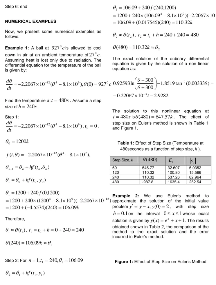
NUMERICAL EXAMPLES
Now, we present some numerical examples as follows:
Example 1: A ball at
927
0c
is allowed to cool down in air at an ambient temperature of27
0c
. Assuming heat is lost only due to radiation. The differential equation for the temperature of the ball is given by:c
dt
d
12 4 9 0927
)
0
(
),
10
1
.
8
(
10
2067
.
2
Find the temperature at
t
480
s
. Assume a step size ofh
240
s
. Step 1:)
10
1
.
8
(
10
2067
.
2
12 4
9
dt
d
,t
0
0
,k
1200
0
),
10
1
.
8
(
10
2067
.
2
)
,
(
t
12
4
9f
)
,
(
1 n n n n
hf
t
)
,
(
0 0 0 1
hf
t
y
)
1200
,
0
(
240
1200
1
f
)
10
2067
.
2
)(
10
1
.
8
1200
(
240
1200
4
9
12
k
09
.
106
)
240
)(
5574
.
4
(
1200
Therefore, 1
(
t
1)
,t
1
t
0
h
0
240
240
109
.
106
)
240
(
k
Step 2: Forn
1
,
t
1
240
,
1
106
.
09
)
,
(
1 1 1 2
hf
t
y
)
1200
,
240
(
240
09
.
106
1
f
)
10
2067
.
2
)(
10
1
.
8
09
.
106
(
240
1200
4
9
12
k
32
.
110
)
240
)(
017545
.
0
(
09
.
106
2
(
t
2)
,t
2
t
1
h
240
240
480
232
.
110
)
480
(
k
The exact solution of the ordinary differential equation is given by the solution of a non linear equation as:
9282
.
2
10
22067
.
0
)
00333
.
0
(
tan
8519
.
1
300
300
ln
92593
.
0
3 1
t
The solution to this nonlinear equation at
s
t
480
is
(
480
)
647
.
57
k
. The effect of step size on Euler’s method is shown in Table 1 and Figure 1.Table 1: Effect of Step Size (Temperature at 480seconds as a function of step size,
h
).Step Size,
h
(
480
)
E
t t
60 546.77 32.607 5.0352 120 110.32 100.80 15.566 240 110.32 537.26 82.964 480 -987.8 1635.4 252.54Example 2: We use Euler’s method to
approximate the solution of the initial value problem
y
y
x
,
y
(
0
)
2
, with step size1
.
0
h
on the interval0
x
1
whose exact solution is given byy
(
x
)
e
x
x
1
. The results obtained shown in Table 2, the comparison of the method to the exact solution and the error incurred in Euler’s method.Table 2: The Comparative Result Analysis and Error generated from Euler’s Method.
n
nx
y
ny
(
x
n)
e
n
y
(
x
n)
y
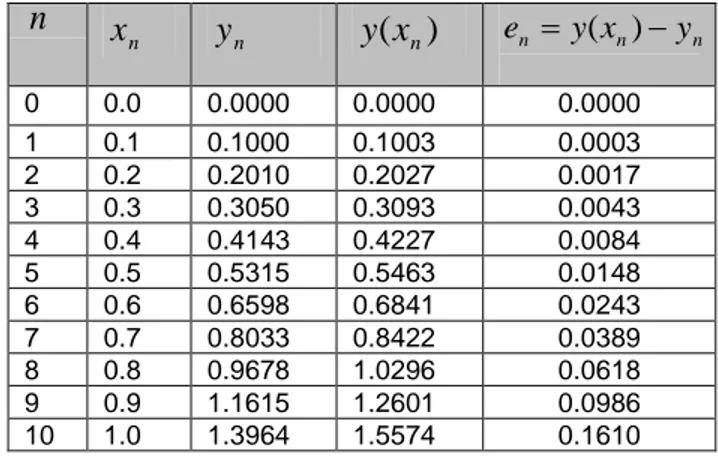
n 0 0.0 2.0000 2.0000 0.0000 1 0.1 2.2000 2.2052 0.0052 2 0.2 2.4100 2.4214 0.0114 3 0.3 2.6310 2.6498 0.0188 4 0.4 2.8641 2.8918 0.0277 5 0.5 3.1105 3.1487 0.0382 6 0.6 3.3716 3.4221 0.0505 7 0.7 3.6487 3.7137 0.0650 8 0.8 3.9436 4.0255 0.0819 9 0.9 4.2579 4.3596 0.1017 10 1.0 4.5937 4.7182 0.1245Example 3: We shall approximate the solution of the initial value problem
y
1
y
2,y
(
0
)
2
using Euler’s method with step size
h
0
.
1
on the interval0
x
1
whose exact solution is given byy
(
x
)
tan
x
. The results obtained shown in Table 3, the comparison of the method to the exact solution and the error incurred in Euler’s method.DISCUSSION OF RESULTS
We notice that in example 1, the accuracy of the approximations gets worse as we further away from the initial value and in examples 2 and 3, the error get larger as
n
increases.Table 3: The Comparative Result Analysis and Error generated from Euler’s Method.
n
nx
y
ny
(
x
n)
e
n
y
(
x
n)
y
n 0 0.0 0.0000 0.0000 0.0000 1 0.1 0.1000 0.1003 0.0003 2 0.2 0.2010 0.2027 0.0017 3 0.3 0.3050 0.3093 0.0043 4 0.4 0.4143 0.4227 0.0084 5 0.5 0.5315 0.5463 0.0148 6 0.6 0.6598 0.6841 0.0243 7 0.7 0.8033 0.8422 0.0389 8 0.8 0.9678 1.0296 0.0618 9 0.9 1.1615 1.2601 0.0986 10 1.0 1.3964 1.5574 0.1610 CONCLUSIONIn general, each numerical method has its own advantages and disadvantages of use: Euler’s method is therefore best reserved for simple preferably, recursive derivatives that can be represented by few terms. It is simple to implement and simplifies rigorous analysis. The major disadvantages of this method are the tiresome, sometimes impossible calculation of higher derivatives and the slow convergence of the series for some functions which involves terms of opposite sign.
REFERENCES
1. Boyce, W.E. and R.C. DiPrima. 2001. Elementary Differential Equation and Boundary Value Problems. John Wiley and Sons: New York, NY.
2. Collatz, L. 1960. Numerical Treatment of Differential Equations. Springer Verlag: Berlin, Germany.
3. Erwin, K. 2003. Advanced Engineering Mathematics. Eighth Edition. Wiley Publishers: New York, NY.
4. Gilat, A. 2004. Matlab: An Introduction with Application. John Wiley and Sons: New York, NY.
5. Kockler, N. 1994. Numerical Methods and Scientific Computing. Clarendon Press: Oxford, UK.
6. Lambert, J.D. 1991. Numerical Method for Ordinary Systems of Initial Value Problems. John Wiley and Sons: New York, NY.
7. Samuel, D.C. 1981. Elementary Numerical Analysis: An Algorithm Approach. Third Edition. Mc Graw International Book Company: New York, NY.
8. Stephen, M.P. 1983. To Compute Numerically, Concepts and Strategy. Little Brown and Company. Ottawa, Canada.
ABOUT THE AUTHORS
Sunday Fadugba, is a Lecturer in the Department of Mathematical and Physical Sciences, Afe Babalola University, Ado Ekiti, Nigeria. He is a registered member of Journal of Mathematical Finance. He holds a Master of Science (M.Sc.) in Mathematics from the University of Ibadan, Nigeria. His research interests are in Numerical Analysis and Financial Mathematics.
Dr. (Mrs.) Bosede Ogunrinde, is a Lecturer I in the Department of Mathematical Sciences, Ekiti State University, Ado Ekiti, Nigeria. She holds a Ph.D. degree in Mathematics. Her research interests are in Ordinary Differential Equations and Numerical Analysis.
Tayo Okunlola, is a Lecturer in the Department of Mathematical and Physical Sciences, Afe Babalola University, Ado Ekiti, Nigeria. He holds a Master of Science in Mathematics from University of Ibadan, Nigeria. His research interest is in Numerical Analysis.
SUGGESTED CITATION
Fadugba, S., B. Ogunrinde, and T. Okunlola. 2012. “Euler’s Method for Solving Initial Value Problems in Ordinary Differential Equations”.
Pacific Journal of Science and Technology. 13(2):152-158.