Euro Area Imbalances
Mark Mink
Jan P.A.M. Jacobs
Jakob de Haan
CESIFO WORKING PAPER NO. 6291
C
ATEGORY7:
M
ONETARYP
OLICY ANDI
NTERNATIONALF
INANCED
ECEMBER2016
Presented at CESifo Area Conference on Macro, Money & International Finance, February 2016
An electronic version of the paper may be downloaded
• from the SSRN website: www.SSRN.com
• from the RePEc website: www.RePEc.org
CESifo Working Paper No. 6291
Euro Area Imbalances
Abstract
We argue that if currency union member states have different potential output per capita, output growth rates, or trade balances, the common monetary policy may not be optimal for all of them. Euro area imbalances for potential output and for trade balances are quite large, while output growth imbalances are more modest. Member states with larger imbalances of one type also have larger imbalances of both other types, but a decline of one imbalance need not coincide with a decline of the others. We also show that imbalances are fairly persistent, and are larger in poorer and smaller member states.
JEL-Codes: E300, F450, O470.
Keywords: euro area macroeconomic imbalances, common monetary policy, economic convergence, business cycle synchronization, euro crisis.
Mark Mink*
De Nederlandsche Bank (DNB) P.O. Box 98
The Netherlands – 1000 AB Amsterdam [email protected]
Jan P.A.M. Jacobs University of Groningen Faculty of Economics and Business The Netherlands – 9747 AE Groningen
[email protected] Jakob de Haan
University of Groningen Faculty of Economics and Business The Netherlands – 9747 AE Groningen
*corresponding author
December 22, 2016
We thank Nikki Panjer for excellent research assistance, and appreciate valuable comments by Niels Gilbert, Jeroen Hessel, Sebastiaan Pool, and participants at the 2016 CESifo Area Conference on Macro, Money & International Finance and at the 2016 ECB Surveillance
1
Introduction
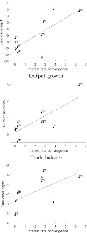
Euro area member states that experienced stronger interest rate declines before the in-troduction of the common monetary policy were hit harder by the recent euro crisis. In particular, as is shown in Figure 1, these countries faced sharper adjustments of their trade balances combined with larger declines of potential output per capita and of output growth. This pattern suggests that the convergence of countries’ interest rates did not coincide with an equal convergence of their macroeconomic fundamentals. Motivated by this observation, we first discuss which economic fundamentals would need to converge if the common monetary policy in a currency union is to be optimal for all member states, and then examine whether this convergence has taken place in the euro area.
One common interpretation of economic convergence is the process where low-income countries catch-up with high-income ones (e.g., Barro and Sala-i-Martin (2002)). Such a process implies that countries with relatively low potential output per capita have relatively high trade deficits and output growth rates. According to several authors (e.g., Buti and Sapir (1998)), the common currency would facilitate such catching-up.1 However, a recent analysis by the European Central Bank (2015) shows that catching-up amongst member states of the euro area has been much weaker than amongst countries elsewhere in the European Union.
Using a simple conceptual framework inspired by the open economy model of Gal´ı and Monacelli (2005), we show that within a currency union macroeconomic differences between member states related to catch-up effects may also lead to differences between their optimal monetary policy interest rates. For example, differences between member
1A common view was that balances-of-payments of individual euro area member states would become
as irrelevant as among regions within a country (e.g., Blanchard and Giavazzi (2002)). Yet the euro crisis has challenged this view (e.g., Holinski, Kool, and Muysken (2012) and Merler and Pisani-Ferry (2012)). Mongelli and Wyplosz (2008) argue that the divergence of trade balances in the euro area may reflect the ‘Walters critique’, which states that a common monetary policy in a currency union has different real effects in member states with different inflation rates.
Potential output
Output growth
Trade balance
Figure 1: Interest rate convergence and the euro crisis. Note: interest rate convergence is measured as the absolute value of the percentage point change in the nominal 3-month money market interest rate during the two years preceding euro area membership (Greece joined in 2001 and the other countries joined in 1999). The depth of the euro crisis is measured as average pre-crisis (1999Q1–2009Q4, and 2001Q1-2009Q4 for Greece) minus average post-crisis (2010Q1–2015Q4) potential output per capita, output growth, and the trade balance (the latter with inverted y-axis, as a larger improvement of the trade balance implies a
states’ potential output per capita can give rise to differences between their natural rates of interest, in which case a common monetary policy can end up being restrictive for some member states while being expansionary for others.2 We provide some empirical support for this theoretical result by showing that before countries joined the euro area, cross-country differences with respect to i) potential output per capita, ii) output growth rates and iii) trade balances can reasonably well account for cross-country differences in interest rates. Hence, a common monetary policy interest rate may only be optimal for all individual member states of a currency union once catching-up processes have been completed. Our empirical analysis therefore examines to what extent euro area member states differ in terms of potential output per capita, output growth rates, and trade balances. To reflect that such differences may pose a problem when implementing a common monetary policy, we refer to them as ‘imbalances’.3
To examine imbalances in euro area member states during the 1999Q1–2015Q4 time period, we adapt one of the measures that Mink, Jacobs and De Haan (2012) propose to analyze the similarity of business cycles. The flexible empirical approach put forward by these authors allows us to measure imbalances at the level of individual member states as well as at the level of the euro area as a whole, both on a per-observation basis.
Our main findings can be summarized as follows. First, output growth imbalances in the euro area seem relatively modest, but imbalances for the trade balance and, particularly, for potential output per capita are considerably larger. While imbalances for the trade balance are currently about as high as at the start of the euro area, imbalances for potential output have grown substantially over time. Second, member states having one type of imbalance
2The empirical work by Laubach and Williams (2003) shows that the natural rate of interest depends
on trend output growth, which Barro and Sala-i-Martin (2002) show is typically higher in countries with lower potential output per capita.
3Note that this definition implies that if all member states of a currency union face the same trade
deficit, there is no ‘imbalance’ between them. Our definition of an imbalance thereby focuses on whether member states’ macroeconomic developments are sufficiently similar to implement a common monetary policy, rather than on whether macroeconomic developments in individual member states are sustainable.
have larger imbalances of the other two types as well, but there is no such correlation in the time dimension. In other words, a decline of one imbalance does not necessarily coincide with a decline of the others. Third, imbalances are fairly persistent over time, so that the core-periphery structure of the euro area has remained largely unchanged after the introduction of the euro. For all three macroeconomic variables examined, relatively large imbalances exist in Greece, Ireland, Portugal and Spain. Fourth, imbalances are larger in member states with lower potential output per capita and a smaller population size. This result implies that imbalances and their adjustment may place a relatively large burden on poorer and smaller member states.
The issue of the optimality of a common monetary policy has been raised before in the empirical literature on optimum currency areas, which focused on the synchronization of shocks and business cycles (see De Haan, Inklaar and Jong-a-Pin (2008) for a survey). In their seminal paper, Bayoumi and Eichengreen (1993) show that before the start of the euro area there was a core of countries where shocks are highly synchronized, and a periphery where synchronization is significantly lower. In their update of the Bayoumi-Eichengreen study, Campos and Macchiarelli (2016) reach more optimistic conclusions. Using the same estimation methodology, sample of countries, and number of time periods, they study the 1989–2015 period and conclude that the core-periphery pattern has weakened. Likewise, following Frankel and Rose (1998), some studies suggest that business cycles within the euro area have become more synchronized due to increasing trade relationships.4 However,
our analysis shows that when examining the optimality of a common monetary policy in a currency union, the synchronization of business cycles (which is closely related to our
4Initial studies indicated that this increase in trade relationships would be considerable (e.g., Rose
(2000)). Since then, estimates of the effect of the euro area on trade have become much smaller and more uncertain (e.g., Berger and Nitsch (2008) and Glick and Rose (2015)), although Rose (2016) shows that larger estimates are obtained if more countries and years are included in the sample. Inklaar, Jong-a-Pin and De Haan (2008) find that the positive impact of trade on business cycle synchronization is smaller than previously reported, but G¨achter and Riedl (2014) conclude that the adoption of the euro has increased the synchronization of business cycles above and beyond the effect of higher trade integration.
concept of output growth imbalances) is only part of the story.5 More broadly, our analysis contributes to the literature on the euro crisis as discussed by Gibson, Palivos and Tavlas (2014) and De Haan, Hessel and Gilbert (2014).
The remainder of the paper is organized as follows. Section 2 outlines a simple concep-tual framework of imbalances, Section 3 discusses our measurement approach, Section 4 describes the data, and Section 5 presents our empirical results. The final section concludes.
2
Conceptual framework
Our empirical analysis of imbalances between euro area member states focuses on three key macroeconomic quantities: potential output per capita, output growth rates, and trade balances. This section shows that this selection is consistent with a simple conceptual framework that focuses on how economic differences between euro area member countries can hamper the successful implementation of a common monetary policy. This framework is inspired by the open economy model of Gal´ı and Monacelli’s (2005), in which country
i’s optimal monetary policy interest rate is:
rit=φππit+φxxit+ ¯rti, (1)
where ri
t is country i’s optimal nominal policy interest rate at time t, πti is inflation,
xi
t≡yit−y¯ti is the output gap, defined as the (logarithmic) deviation of per capita outputyit
from its potential value ¯yi
t, ¯rtiis the natural rate of interest, and with parametersφπ, φx >0.
As shown by C´urdia, Ferrero, Ng and Tambalotti (2015), this type of interest rate rule also quite accurately describes monetary policy decisions in practice.
After country i joins the euro area, its monetary policy interest rate is set by the
5De Grauwe and Mongelli (2005) and Estrada, Gal´ı and Lopez-Salido (2013) also focus on a larger set of
variables when assessing euro area economic convergence. The former authors were moderately optimistic, but like the present paper the latter authors identify substantial divergences as well.
European Central Bank. If this policy interest rate is to be optimal for the euro area as a whole as well as for country i individually, it has to be the case that rti = reat . Using (1), this equality can be written as:
φπ(πti−π ea t ) +φx(xit−x ea t ) + (¯r i t−r¯ ea t ) = 0. (2)
The analysis in Gal´ı and Monacelli (2005) shows that this condition can be expressed in terms of the same three variables that are the focus of our empirical analysis. Firstly, the natural rate of interest ¯ri
t in Gal´ı and Monacelli (2005) is a function of potential output, in
such a way that we can write ¯ri
t−r¯eat =−φy¯(¯yit−y¯tea), with reduced form parameterφy¯>0.6
This relationship implies that in the cross-section of countries, those with potential output per capita below the euro area aggregate have a higher natural rate of interest. Substituting this relationship in (2) yields:
φπ(πti−π ea t ) +φx(xit−x ea t )−φy¯(¯yit−y¯ ea t ) = 0. (3)
This expression highlights that even if cyclical fluctuations in country i’s output and in-flation are identical to those for the euro area as a whole, so that the first two terms of the equality are equal to zero, differences between potential output levels may still cause countries to require different monetary policy interest rates.
Secondly, the difference between inflation rates in (3) can be written as a function of the difference between output growth rates, with (logarithmic) output growth being defined as ∆yi
t ≡ yti −yti−1. In particular, the model by Gal´ı and Monacelli (2005) implies that
6More specifically, Gal´ı and Monacelli’s (2005) expression (37) describes country i’s natural rate of
interest as a function of worldwide output growth, the rate of time preference, andi’s productivity. Their expression (35) can then be used to replacei’s productivity byi’s potential output. As worldwide output growth and the rate of time preference are the same across countries, differences between natural rates of interest can therefore be written as a function of differences between potential output, which yields the relationship in the main text.
φπ(πit−πtea) = −φ
0
(∆yti−∆ytea), with reduced form parameterφ0 >0.7 Those countries with a higher output growth rate will thus also experience higher inflation. Thirdly, the model allows us to write differences between output levels as a function of differences between trade balancesnxi
t, using the reduced form relationshipφx(yit−ytea) = φ
00
(nxi
t−nxeat ), with
φ00 > 0.8 This relationship implies that countries with per capita output above the euro
area aggregate have a higher trade balance. Using this result after substitutingxi
t≡yit−y¯it
into (3) yields:
−φ0(∆yit−∆ytea) +φ00(nxit−nxeat )−φ000(¯yit−y¯eat ) = 0, (4)
whereφ000 ≡φy¯+φx. This result does not imply any causal relationship, in one direction or
the other, between optimal monetary policy interest rates and potential output per capita, output growth rates, and the trade balance. However, it does illustrate that if:
∆yti−∆ytea = 0, (5)
nxit−nxeat = 0, (6)
¯
yti−y¯tea = 0, (7)
the policy interest rate that is optimal for the euro area as a whole is also optimal for its individual member states. In this case, the European Central Bank can set its interest rate
7This result uses Gal´ı and Monacelli’s (2005) expression (29) to write countryi’s output growth as a
function of worldwide output growth and of the change in countryi’s terms of trade. Worldwide output growth is the same for all countries, and changes in the terms of trade, as follows from the authors’ expression (15), depend on country i’s inflation, on worldwide inflation, and on changes in country i’s exchange rate. These last two variables are the same for all countries if they share a common currency, which yields the reduced form expression in the main text that relates output growth differences between countries to differences between their inflation rates.
8This result again reflects Gal´ı and Monacelli’s (2005) expression (29), which relates countryi’s output
to worldwide output and to country i’s terms of trade. With worldwide output being the same for all countries, using the authors’ expression (31) to relate the terms of trade to the trade balance suffices to write differences between output levels as a function of differences between trade balances. This yields the reduced form relationship in the main text.
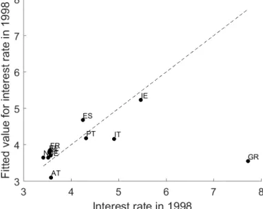
Figure 2: Interest rates before monetary unification. Note: the horizontal axis displays the 3-month nominal interest rate in the year before a country joined the euro area (which they all did in 1999, except for Greece which joined in 2001). The vertical axis displays the fitted value obtained from a robust least squares regression of the cross-section of interest rates on the contemporaneously observed values for potential output per capita, output growth rates, and trade balances (using robust least squares takes into account that Greece clearly is an outlier). A dashed 45-degree line is displayed as well.
at this optimal level, thereby ensuring that its monetary policy suits all euro area member states. By contrast, if these equalities do not hold, optimal monetary policy interest rates may differ across countries. Figure 2 provides some empirical support for this notion, by showing that the variation in interest rates across member states before the introduction of the euro is reasonably well explained by the variation in their potential output per capita, output growth rates, and trade balances. Our empirical analysis therefore focuses on deviations from equalities (5)-(7) within the euro area.
3
Measuring imbalances
To measure the imbalance for a variableztacrossN ≥2 euro area member states, we adapt
calculate: Iz,tea ≡ 1 N N X i=1 |zit−zeat |, with z = ∆y, nx,y¯ (8)
where zeat is the reference value for the euro area as a whole, calculated as the median
value of zi
t in the N euro area member states. This imbalance measure is equal to the
cross-country average of imbalances at the individual country level, which we calculate as Ii
z,t ≡ |zti−ztea|. The euro area imbalance Iz,tea is at its minimum value of 0 if zit’s are
identical across all N member states. Higher values indicate that imbalances observed at time t are larger. One of the advantages of this measure is that it can be calculated at each point in time rather than that it needs to be calculated for a longer sample period. Consequently, the variation of imbalances in the cross-section of countries can be analyzed separately from the variation of imbalances over time.
4
Data
We use time series for the growth rate of output ∆y, the trade balance as a percentage of output nx, and potential output per capita ¯y. The data for output growth and the trade balance are from Eurostat, the data for potential output has been obtained from the Eu-ropean Commission’s Ameco Database. Our sample consists of Austria, Belgium, Finland, France, Germany, Greece, Ireland, Italy, Netherlands, Portugal, and Spain. For each of these countries, time series data are available for the period 1999Q1 to 2015Q4. Data on output growth and the trade balance are available at a quarterly frequency. However, data for potential output is only available on an annual basis, so that we linearly interpolated the series to obtain data at a quarterly frequency.9
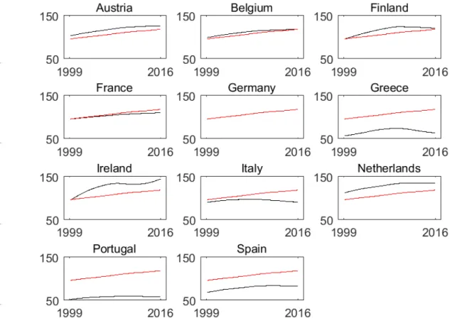
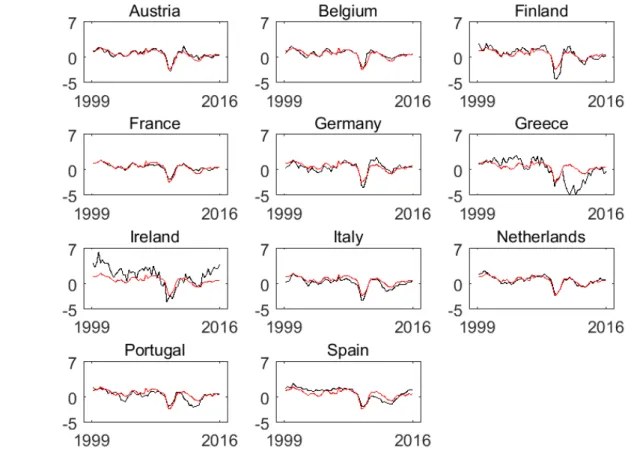
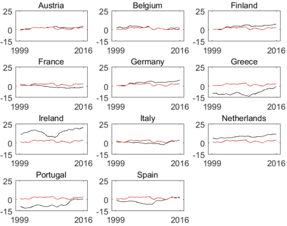
Figures 3 to 5 show the development of our three key variables over time. The blue
9We normalized potential output per capita such that its average over all euro area inhabitants and all
lines indicate the time series for each individual country, while the red line indicates the euro area reference (i.e., the cross-country median, as discussed above). Figure 3 shows that Greece, Italy, Portugal, and Spain have relatively low potential output. With respect to output growth rates, Figure 4 shows that especially Greece and Ireland differ frequently from the euro area reference. Finally, Figure 5 shows countries’ trade balances, which tend to be relatively low in Greece, Portugal, and Spain, while they tend to be relatively high in Finland, Ireland, the Netherlands, and Germany.
5
Empirical analysis
We next examine how imbalances within the euro area evolved since the start of the currency union. Thereafter, we analyze to what extent imbalances are related in both the country and the time dimension. Finally we focus on the persistence of imbalances and the characteristics of countries where imbalances are relatively large.
5.1
Are imbalances large?
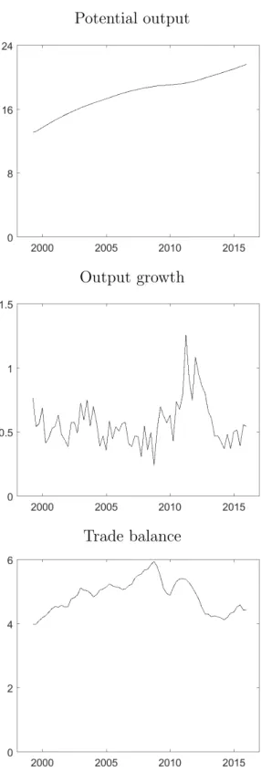
Figure 6 displays imbalances at the level of the euro area as a whole, calculated using the measure Iz,tea in (8). The underlying imbalances for individual member states, calculated using the measure Ii
z,t, are shown in Appendix A. The graph in the top panel in Figure 6
shows that potential output imbalances within the euro area increased considerably. The imbalance value of 22 in 2015 is quite high, as potential output per capita averaged over all euro area inhabitants and time periods was normalized to equal 100. This result illustrates that poorer member states have not been catching-up with richer ones.
The graph in the middle of Figure 6 shows that euro area imbalances in output growth declined somewhat after the start of the currency union, but the financial crisis in 2007 caused imbalances to increase substantially. This result reflects that the recession following
Figure 3: Potential output per capita. Note: the black lines indicate national potential output per capita levels, while the red line indicates the reference value for the euro area as a whole.
Figure 4: Output growth. Note: the black lines indicate national output growth rates, while the red line indicates the reference value for the euro area as a whole.
Figure 5: Trade balances. Note: the black lines indicate national trade balances as a percentage of output, while the red line indicates the reference value for the euro area as a whole.
Potential output
Output growth
Trade balance
Figure 6: Euro area imbalances. Note: the graphs show imbalances within the euro area as a whole, calculated using Iz,tea in (8). The upper panel displays potential output imbalances, the middle panel displays output growth imbalances, and the lower panel displays trade imbalances.
the crisis affected some countries much harder than others. More recently, output growth imbalances have come down, so that nowadays they are about as large as at the start of the euro area. Overall, there is no strong evidence for a downward trend in output growth imbalances over time.
The graph in the panel at the bottom in Figure 6 shows that trade imbalances were already high at the start of the currency union and increased further during the first years thereafter. The large trade deficits of some countries increased their external indebtedness, which proved unsustainable during the euro crisis. Since then, trade imbalances have started to decrease, which is mainly due to adjustments in Greece, Portugal, and Spain as shown by Figure 5. By contrast, trade balances for Ireland and the Netherlands have consistently been above the euro area reference.
In order to compare the relative magnitude of the imbalances shown in Figure 6, we convert the three imbalance measures to the same scale by calculating the absolute values of all quarterly changes in an imbalance measure over the 1999Q1-2015Q4 period, and then divide the level of the imbalance at the end of the sample by the average of these absolute values. This way, we obtain an indicator of how much time it would take for a current imbalance to become equal to zero in the hypothetical case that it would from now on decline every quarter by an amount equal to the typical change in the imbalance observed in the past. Accordingly, output growth imbalances would become equal to zero in just a little more than one year from now. Imbalances for the trade balance, however, would become equal to zero more than eleven years from now, while potential output imbalances would become equal to zero after almost forty-three years. Viewed this way, imbalances in potential output and in trade balances seem to be particularly large, while those in output growth rates seem relatively modest.
It has been argued that the currency union would help poorer member states to catch-up with richer ones. For instance, according to Buti and Sapir (1998), a “single European
currency has the advantage of reducing transaction costs on goods and factor markets between participating countries. This effect will turn out higher in the peripheral Member States than in the core Member States and will, if accompanied by sound economic policies, favour the process of income convergence.” A catch-up process implies that countries with lower potential output levels have higher trade deficits and higher output growth rates (e.g., Blanchard and Giavazzi (2002)). Figure 7 shows that there has been no such patter in the euro area: member states with lower potential output experienced lower trade balances, but these lower trade balances were associated with lower (rather than higher) output growth rates. Consequently, potential output differences in the euro area have consistently grown over time, as was illustrated by the graph in the top panel of Figure 6.
5.2
Are imbalances related?
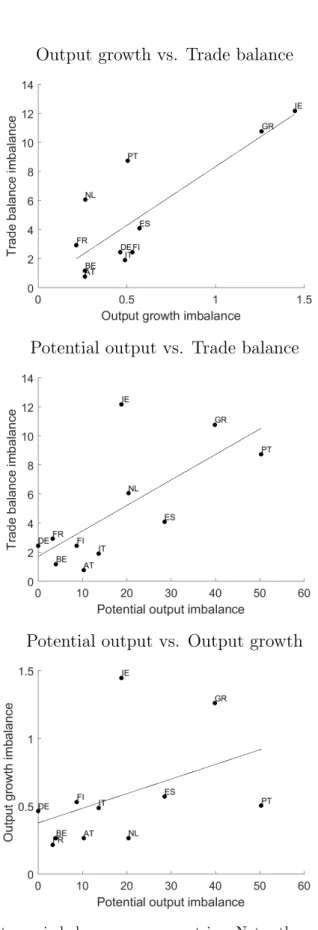
Figure 8 shows that all three types of imbalances are positively related in the country dimension. The graph in the top panel in the figure shows that countries with a small output growth imbalance also tend to have a small imbalance for the trade balance. The graph in the panel in the middle shows that a similar positive relationship exists between potential output imbalances and imbalances for the trade balance, while the graph in the bottom panel of the figure displays such a relationship for output growth imbalances and potential output imbalances. Hence, countries that do well in terms of one imbalance measure also tend to do well in terms of the two others.
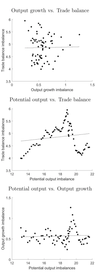
Figure 8 might suggest that policymakers do not face difficult trade-offs in reducing imbalances within the euro area, as redressing one imbalance may also help reducing others. Unfortunately, this conclusion turns out too good to be true. As Figure 9 shows, the positive relationship between imbalances that holds in the country dimension does not hold in the time dimension. That is, quarters associated with low imbalances of one type are not associated with low imbalances of the other two types. This result suggests that
Trade balance vs. Potential output
Trade balance vs. Output growth
Figure 7: No catch-up effect. Note: the top graph displays the relationship between potential output per capita and the trade balance, while the bottom graph displays the relationship between the trade balance and output growth rates. For each variable, a country’s time series with quarterly observations was expressed in deviation from the corresponding time series with euro area median values, and was then averaged over time.
Output growth vs. Trade balance
Potential output vs. Trade balance
Potential output vs. Output growth
Figure 8: Relationship between imbalances across countries. Note: the graphs indicate to what extent countries that experience higher imbalances of one type experience higher imbalances of the other two types as well.
a reduction of one type of imbalance within the euro area may coincide with an increase in another type of imbalance. Needless to say, such a relationship would complicate policy makers’ efforts to achieve an overall reduction of imbalances within the area.
5.3
Are imbalances persistent?
The results so far suggest that there is no strong tendency for imbalances in the euro area to decline since the start of the currency union. This observation is confirmed by Figure 10, which relates countries’ imbalances in 1998, i.e., in the year before the introduction of the euro, to their imbalances during the years thereafter. The figure shows that countries which entered the monetary union with relatively large imbalances had higher imbalances thereafter as well. Moreover, the graphs confirm the common view that the euro area ‘periphery’ is comprised of Greece, Ireland, Portugal, and Spain (i.e., the GIPS), as these countries are in the top five of member states with the highest imbalance for each of the three macroeconomic variables.
5.3.1 Imbalances are larger in poorer member states
One country characteristic that is associated with larger imbalances is initial potential output per capita. As is shown by Figure 11, countries with lower potential output at the start of the euro area had higher imbalances during the period thereafter. As such imbalances may imply that these countries require a different monetary policy interest rate than the euro area as a whole, the common monetary policy could have been less optimal for poorer member states. On a more positive note, the figure suggests that if poorer countries’ are able to increase their potential output levels, for instance by introducing structural reforms, this may reduce their other imbalances as well.
Output growth vs. Trade balance
Potential output vs. Trade balance
Potential output vs. Output growth
Figure 9: Relationship between imbalances over time. Note: the graphs indicate to what extent quarters characterized by higher imbalances of one type are characterized by higher imbalances of the other two types as well.
Potential output
Output growth
Trade balance
Figure 10: Persistence of imbalances. Note: the graphs indicate to what extent countries’ imbalances in 1998 are related to their imbalances over 1999–2016.
Potential output
Output growth
Trade balance
Figure 11: Imbalances and initial potential output. Note: the graphs indicate to what extent imbalances over 1999–2016 are related to countries’ 1998 potential output per capita (in thousands of euros).
5.3.2 Imbalances are larger in smaller member states
Country size does not play a role in any of our imbalances measures (our variables are expressed in per-capita terms or as percentages of output levels, and the cross-country median values used to calculate the imbalance measures do not depend on country size either). Still, Figure 12 shows that countries with a smaller population size in 1998 tended to have larger imbalances thereafter. This observation may reflect that economic develop-ments in a large country such as Germany have a larger impact on other member states than economic developments in a small country such as Greece. But if countries’ indi-vidual imbalances are indeed associated with a time-invariant factor such as population size, reducing imbalances in the euro area may prove to be a difficult task which places a relatively large burden on smaller member states.
6
Conclusion
Since the euro area was established in 1999, there have been considerable differences be-tween its member states with respect to i) potential output per capita, ii) output growth rates, and iii) trade balances. While such imbalances are typically associated with low-income countries catching-up with richer ones, we show that in a currency union they may also undermine the optimality of a common monetary policy for individual member states. Imbalances in the euro area are the largest for potential output per capita and for trade balances, while output growth imbalances have generally been more modest. When member states have larger imbalances of one type they also tend to have larger imbalances of both other types, but a decline of one imbalance need not coincide with a decline of the others. All three types of imbalances have been especially large in Greece, Ireland, Portugal, and Spain. Moreover, imbalances tend to be fairly persistent, and are larger in member states which have a lower level of potential output per capita and a smaller
Potential output
Output growth
Trade balance
Figure 12: Imbalances and initial population size. Note: the graphs indicate to what extent imbalances over 1999–2016 are related to countries’ 1998 population size (in millions of inhabitants).
population size. This finding suggests that the common monetary policy may have been less optimal for poorer and smaller member states.
One question raised by our analysis is whether the catching-up of poorer euro area member states with richer ones is hampered by the common monetary policy. The Eu-ropean Central Bank (2015) shows that catch-up processes in the euro area were much weaker than elsewhere in the European Union. Our analysis suggests that the negative consequences of such catching-up for the optimality of a common monetary policy may be related to this difference. For example, if poorer euro area member states which grow faster due to catching-up have a higher natural rate of interest, the common monetary policy interest rate is likely to be too low for them. These low interest rates may, in turn, affect their growth potential. For instance, F´ernandez-Villaverde, Garicano and Santos (2013) show that such low interest rates may cause countries to postpone structural re-forms that would enhance productivity, while Benigno and Fornaro (2014) and Gilbert and Pool (2016) show that they may trigger a consumption boom and a reallocation of resources to the less productive non-tradables sector. It remains an open question to what extent the consequences of the euro area’s imbalances for the optimality of its common monetary policy may explain the different catch-up processes inside and outside the euro area. This we leave for future research.
References
Barro, R.J. and X. Sala-i-Martin (1992), Convergence. Journal of Political Economy, 100, p. 223–51.
Bayoumi, T. and B. Eichengreen (1993), Shocking Aspects of European Monetary Inte-gration. In: F. Torres and F. Giavazzi (eds),Adjustment and Growth in the European
Monetary Union, Cambridge University Press.
Benigno, G. and L. Fornaro (2014), The Financial Resource Curse. The Scandinavian Journal of Economics, 116, p. 58-86.
Berger, H. and V. Nitsch (2008), Zooming Out: The Trade Effect of the Euro in Historical Perspective. Journal of International Money and Finance, 27, p. 1244–60.
Blanchard, O. and F. Giavazzi (2002), Current Account Deficits in the Euro Area: The End of the Feldstein-Horioka Puzzle? Brookings Papers on Economic Activity, 33, p. 147–86.
Buti, M. and A. Sapir (eds.) (1998),Economic Policy in EMU, Clarendon Press.
Campos, N.F. and C. Macchiarelli (2016), Core and Periphery in the European Monetary Union: Bayoumi and Eichengreen 25 Years Later. Economics Letters, 147, p. 127–30.
C´urdia, V, Ferrero, A., Ng, G. and A. Tambalotti (2015), Has U.S. Monetary Policy Tracked the Efficient Interest Rate? Journal of Monetary Economics, 70, p. 72–83.
De Grauwe, P. and F.P. Mongelli (2005), Endogeneities of Optimum Currency Areas -What Brings Countries Sharing a Single Currency Closer Together? ECB Working
De Haan, J., J. Hessel and N. Gilbert (2014), Reforming the Architecture of EMU: En-suring Stability in Europe. In: Badinger, H. and V. Nitsch (eds.), Handbook of the
Economics of European Integration, Routledge.
De Haan, J., R. Inklaar and R.M. Jong-a-Pin (2008), Will Business Cycles in the Euro Area Converge? A Critical Survey of Empirical Research. Journal of Economic Surveys, 22, p. 234–73.
European Central Bank (2015), Real Convergence in the Euro Area: Evidence, Theory and Policy Implications. ECB Economics Bulletin, 5, p. 30–45.
Estrada, A., J. Gal´ı, and D. Lopez-Salido (2013), Patterns of Convergence and Divergence in the Euro Area. IMF Economic Review, 61, p. 601–30.
F´eernandez-Villaverde, J., L. Garicano and T. Santos (2013), Political Credit Cycles: The Case of the Eurozone. The Journal of Economic Perspectives, 27, p. 145–66.
Frankel, J.A. and A.K. Rose (1998), The Endogeneity of the Optimum Currency Area Criteria. The Economic Journal, 108, p. 1009–25.
G¨achter, M. and A. Riedl (2014), One Money, One Cycle? The EMU Experience. Journal of Macroeconomics, 42, p. 141–55.
Gal´ı, J. and T. Monacelli (2005), Monetary Policy and Exchange Rate Volatility in a Small Open Economy. The Review of Economic Studies, 72, p. 707–34.
Gibson, H.D., T. Palivos and G.S. Tavlas (2014), The Crisis in the Euro Area. Papers Presented at a Bank of Greece Conference. Journal of Macroeconomics, 39, p. 233– 460.
Gilbert, N. and S. Pool (2016), Sectoral Allocation and Macroeconomic Imbalances in
Glick, R. and A.K. Rose (2015), Currency unions and trade: A post-EMU mea culpa.
NBER Working Paper 21535.
Holinski, N, C. Kool and J. Muysken (2012), Persistent Macroeconomic Imbalances in the Euro Area: Causes and Consequences. Federal Reserve Bank of St. Louis Review, 94, p. 1–20.
Inklaar, R., R. Jong-a-Pin and J. de Haan (2008), Trade and Business Cycle Synchro-nization in OECD Countries A Re-examination. European Economic Review, 52, p. 646–66.
Laubach, T. and J.C. Williams (2003), Measuring the Natural Rate of Interest. The Review of Economics and Statistics, 85, p. 1063–70.
Merler, S. and J. Pisani-Ferry (2012), Sudden Stops in the Euro Area. Bruegel Policy Contribution 6.
Mink, M., J.P.A.M. Jacobs, and J. de Haan (2012), Measuring Coherence of Output Gaps with an Application to the Euro Area.Oxford Economic Papers, 64, p. 217–36.
Mongelli, F.P. and C. Wyplosz (2008), The Euro at Ten: Unfulfilled Threats and Unex-pected Challenges. Fifth ECB Central Banking Conference, European Central Bank.
Rose, A.K. (2000), One Money, One Market: The Effect of Common Currencies on Trade.
Economic Policy, 15, p. 7–45.
Rose, A. K. (2016), Why Do Estimates of the EMU Effect On Trade Vary so Much? Open
A
Imbalances by country over time
Figure A.1: National potential output imbalances. Note: the graphs indicate the development over time of potential output imbalances for individual countries.
Figure A.2: National output growth imbalances. Note: the graphs indicate the development over time of output growth imbalances for individual countries.
Figure A.3: National trade balance imbalances. Note: the graphs indicate the development over time of trade balance imbalances for individual countries.