arXiv:1502.07989v2 [stat.CO] 28 Oct 2015
Statistical Methods and Computing for Big Data
Chun Wang, Ming-Hui Chen, Elizabeth Schifano, Jing Wu, and Jun Yan
October 29, 2015
Abstract
Big data are data on a massive scale in terms of volume, intensity, and complexity that exceed the capacity of standard analytic tools. They present opportunities as well as challenges to statisticians. The role of computational statisticians in scientific discovery from big data analyses has been under-recognized even by peer statisticians. This article summarizes recent methodological and software developments in statistics that address the big data challenges. Methodologies are grouped into three classes: subsampling-based, divide and conquer, and online updating for stream data. As a new contribution, the online updating approach is extended to variable selection with commonly used criteria, and their performances are assessed in a simulation study with stream data. Software packages are summarized with focuses on the open source R and Rpackages, covering recent tools that help break the barriers of computer memory and computing power. Some of the tools are illustrated in a case study with a logistic regression for the chance of airline delay.
Key words: bootstrap; divide and conquer; external memory algorithm; high perfor-mance computing; online update; sampling; software;
1
Introduction
A 2011 McKinsey report predicted shortage of talent necessary for organizations to take advantage of big data (Manyika et al., 2011). Data now stream from daily life thanks to technological advances, and big data has indeed become a big deal (e.g., Shaw, 2014). In the President’s Corner of the June 2013 issue of AMStat News, the three presidents (elect, current, and past) of the American Statistical Association (ASA) wrote an article titled “The ASA and Big Data” (Schenker et al., 2013). This article echos the June 2012 col-umn of Rodriguez (2012) on the recent media focus on big data, and discusses on what the statistics profession needs to do in response to the fact that statistics and statisti-cians are missing from big data discussions. In the followup July 2013 column, president Marie Davidian further raised the issues of statistics not being recognized as data science and mainstream academic statisticians being left behind by the rise of big data (Davidian, 2013). A white paper prepared by a working group of the ASA called for more ambitious efforts from statisticians to work together with researchers in other fields on national re-search priorities in order to achieve better science more quickly (Rudin et al., 2014). The
same concern was expressed in a 2014 president’s address of the Institute of Mathemat-ical Statistics (IMS) (Yu, 2014). President Bin Yu of the IMS called for statisticians to own Data Science by working on real problems such as those from genomics, neuroscience, astronomy, nanoscience, computational social science, personalized medicine/healthcare, finance, and government; relevant methodology/theory will follow naturally.
Big data in the media or the business world may mean differently than what are familiar to academic statisticians (Jordan and Lin, 2014). Big data are data on a massive scale in terms of volume, intensity, and complexity that exceed the ability of standard software tools to manage and analyze (e.g., Snijders et al., 2012). The origin of the term “big data” as it is understood today has been traced back in a recent study (Diebold, 2012) to lunch-table conversations at Silicon Graphics in the mid-1990s, in which John Mashey figured prominently (Mashey, 1998). Big data are generated by countless online interactions among people, transactions between people and systems, and sensor-enabled machinery. Internet search engines (e.g., Google and YouTube) and social network tools (e.g., Facebook and Twitter) generate billions of activity data per day. Rather than Gigabytes and Terabytes, nowadays, the data produced are estimated by zettabytes, and are growing 40% every day (Fan and Bifet, 2013). In the big data analytics world, a 3V definition by Laney (2001) is widely accepted: volume (amount of data), velocity (speed of data in and out), and variety (range of data types and sources). High variety brings nontraditional or even unstructured data types, such as social network sentiments and internet map usage, which calls for new, creative ways to understand the structure of data and even to ask intelligent research questions (e.g., Jordan and Lin, 2014). High volume and high velocity may bring noise accumulation, spurious correlation and incidental homogeneity, creating issues in computational feasibility and algorithmic stability (Fan et al., 2014).
Notwithstanding that new statistical thinking and methods are needed for the high variety aspect of big data, our focus is on fitting standard statistical models to big data whose size exceeds the capacity of a single computer from its high volume and high ve-locity. There are two computational barriers for big data analysis: 1) the data can be too big to hold in a computer’s memory; and 2) the computing task can take too long to wait for the results. These barriers can be approached either with newly developed sta-tistical methodologies and/or computational methodologies. Despite the impression that statisticians are left behind in media discussions or governmental summits on big data, some statisticians have made important contributions and are pushing the frontier. Sound statistical procedures that are scalable computationally to massive datasets have been pro-posed (Jordan, 2013). Examples are subsampling-based approaches (Kleiner et al., 2014; Ma et al., 2013; Liang et al., 2013; Maclaurin and Adams, 2014), divide and conquer ap-proaches (Lin and Xi, 2011; Chen and Xie, 2014; Song and Liang, 2014; Neiswanger et al., 2013), and online updating approaches (Schifano et al., 2015). From a computational per-spective, much effort has been put into the most active, open source statistical environment,
R (R Core Team, 2014a). Statistician R developers are relentless in their drive to extend the reach of Rinto big data (Rickert, 2013). Recent UseR! conferences had many presenta-tions that directly addressed big data, including a 2014 keynote lecture by John Chambers, the inventor of the S language (Chambers, 2014). Most cutting edge methods are first and easily implemented in R. Given the open source nature of R and the active recent
development, our focus on software for big data will be on R and R packages. Revolution
R Enterprise (RRE) is a commercialized version of R, but it offers free academic use, so it is also included in our case study and benchmarked. Other commercial software such as
SAS, SPSS, and MATLAB will be briefly touched upon for completeness.
The rest of the article is organized as follows. Recent methodological developments in statistics on big data are summarized in Section 2. Updating formulas for commonly used variable selection criteria in the online setting are developed and their performances studied in a simulation study in Section 3. Resources from open source software R for analyzing big data with classical models are summarized in Section 4. Commercial software products are presented in Section 5. A case study on a logistic model for the chance of airline delay is presented in Section 6. A discussion concludes in Section 7.
2
Statistical Methods
The recent methodologies for big data can be loosely grouped into three categories: resampling-based, divide and conquer, and online updating. To put the different methods in a context, consider a dataset with n independent and identically distributed observations, where n is too big for standard statistical routines such as logistic regression.
2.1
Subsampling-Based Methods
2.1.1 Bags of Little BootstrapKleiner et al. (2014) proposed the bags of little bootstrap (BLB) approach that provides both point estimates and quality measures such as variance or confidence intervals. It is a combination of subsampling (Politis et al., 1999), the m-out-of-n bootstrap (Bickel et al., 1997), and the bootstrap (Efron, 1979) to achieve computational efficiency. BLB consists of the following steps. First, draw s subsamples of size m from the original data of size n. For each of the s subsets, drawr bootstrap samples of size n instead of m, and obtain the point estimates and their quality measures (e.g., confidence interval) from the r bootstrap sample. Then, the sbootstrap point estimates and quality measures are combined (e.g., by average) to yield the overall point estimates and quality measures. In summary, BLB has two nested procedures: the inner procedure applies the bootstrap to a subsample, and the outer procedure combines these multiple bootstrap estimates. The subsample size m was suggested to be nγ with γ ∈[0.5,1] (Kleiner et al., 2014), a much smaller number than n.
Although the inner bootstrap procedure conceptually generates multiple resampled data of size n, what is really needed in the storage and computation is a sample of size m with a weight vector. In contrast to subsampling and the m-out-of-n bootstrap, there is no need for an analytic correction (e.g., p
m/n) to rescale the confidence intervals from the final result. The BLB procedure facilitates distributed computing by letting each subsample of size mbe processed by a separate processor. Kleiner et al. (2014) proved the consistency of BLB and provided high order correctness. Their simulation study showed good accuracy, convergence rate and the remarkable computational efficiency.
2.1.2 Leveraging
Ma and Sun (2014) proposed to use leveraging to facilitate scientific discoveries from big data using limited computing resources. In a leveraging method, one samples a small pro-portion of the data with certain weights (subsample) from the full sample, and then per-forms intended computations for the full sample using the small subsample as a surrogate. The key to success of the leveraging methods is to construct the weights, the nonuniform sampling probabilities, so that influential data points are sampled with high probabilities (Ma et al., 2013). Leveraging methods are different from the traditional subsampling or
m-out-of-n bootstrap in that 1) they are used to achieve feasible computation even if the simple analytic results are available; 2) they enable visualization of the data when visualiza-tion of the full sample is impossible; and 3) they usually use unequal sampling probabilities for subsampling data. This approach is quite unique in allowing pervasive access to extract information from big data without resorting to high performance computing.
2.1.3 Mean Log-likelihood
Liang et al. (2013) proposed a resampling-based stochastic approximation approach with an application to big geostatistical data. The method uses Monte Carlo averages calculated from subsamples to approximate the quantities needed for the full data. Motivated from minimizing the Kullback–Leibler (KL) divergence, they approximate the KL divergence by averages calculated from subsamples. This leads to a maximum mean log-likelihood estimation method. The solution to the mean score equation is obtained from a stochastic approximation procedure, where at each iteration, the current estimate is updated based on a subsample of sizem drawn from the full data. As mis much smaller thann, the method is scalable to big data. Liang et al. (2013) established the consistency and asymptotic normality of the resulting estimator under mild conditions. In a simulation study, the convergence rate of the method was almost independent of n, the sample size of the full data.
2.1.4 Subsampling-Based MCMC
As a popular general purpose tool for Bayesian inference, Markov chain Monte Carlo (MCMC) for big data is challenging because of the prohibitive cost of likelihood evaluation of every datum at every iteration. Liang and Kim (2013) extended the mean log-likelihood method to a bootstrap Metropolis–Hastings (MH) algorithm in MCMC. The likelihood ra-tio of the proposal and current estimate in the MH rara-tio is replaced with an approximara-tion from the mean log-likelihood based onkbootstrap samples of sizem. The algorithm can be implemented exploiting the embarrassingly parallel structure and avoids repeated scans of the full dataset in iterations. Maclaurin and Adams (2014) proposed an auxiliary variable MCMC algorithm called Firefly Monte Carlo (FlyMC) that only queries the likelihoods of a potentially small subset of the data at each iteration yet simulates from the exact posterior distribution. For each data point, a binary auxiliary variable and a strictly positive lower bound of the likelihood contribution are introduced. The binary variable for each datum effectively turn on and off data points in the posterior, hence the “firefly” name. The
probability of turning on each datum depends on the ratio of its likelihood contribution and the introduced lower bound. The computational gain depends on that the lower bound is tight enough and that simulation of the auxiliary variables is cheap enough. Because of the need to hold the whole data in computer memory, the size of the data this method can handle is limited.
The pseudo-marginal Metropolis–Hasting algorithm replaces the intractable target (pos-terior) density in the MH algorithm with an unbiased estimator (Andrieu and Roberts, 2009). The the log-likelihood is estimated by an unbiased subsampled version, and an un-biased estimator of the likelihood is obtained by correcting the bias of the exponentiation of this estimator. Quiroz et al. (2014) proposed subsampling the data using probability proportional-to-size (PPS) sampling to obtain an approximately unbiased estimate of the likelihood which is used in the M-H acceptance step. The subsampling approach was fur-ther improved in Quiroz et al. (2015) using the efficient and robust difference estimator form the survey sampling literature.
2.2
Divide and Conquer
A divide and conquer algorithm (which may appear under other names such as divide and recombine, split and conquer, or split and merge) generally has three steps: 1) partitions a big dataset into K blocks; 2) processes each block separately (possibly in parallel); and 3) aggregates the solutions from each block to form a final solution to the full data.
2.2.1 Aggregated Estimating Equations
For a linear regression model, the least squares estimator for the regression coefficient β
for the full data can be expressed as a weighted average of the least squares estimator for each block with weight being the inverse of the estimated variance matrix. The success of this method for linear regression depends on the linearity of the estimating equations in β and that the estimating equation for the full data is a simple summation of that for all the blocks. For general nonlinear estimating equations, Lin and Xi (2011) proposed a linear approximation of the estimating equations with the Taylor expansion at the solution in each block, and, hence, reduce the nonlinear estimating equation to the linear case so that the solutions to all the blocks are combined by a weighted average. The weight of each block is the slope matrix of the estimating function at the solution in that block, which is the Fisher information or inverse of the variance matrix if the equations are score equations. Lin and Xi (2011) showed that, under certain technical conditions including K = O(nγ)
for some γ ∈(0,1), the aggregated estimator has the same limit as the estimator from the full data.
2.2.2 Majority Voting
Chen and Xie (2014) consider a divide and conquer approach for generalized linear models (GLM) where both the sample size n and the number of covariates p are large, by incor-porating variable selection via penalized regression into a subset processing step. More specifically, for pbounded or increasing to infinity slowly, (pn not faster than o(enk), while
model size may increase at a rate of o(nk)), they propose to first randomly split the data
of size n into K blocks (size nk = O(n/K)). In step 2, penalized regression is applied
to each block separately with a sparsity-inducing penalty function satisfying certain reg-ularity conditions. This approach can lead to differential variable selection among the blocks, as different blocks of data may result in penalized estimates with different non-zero regression coefficients. Thus, in step 3, the results from the K blocks are combined by majority vote to create a combined estimator. The implicit assumption is that real effects should be found persistently and therefore should be present even under perturbation by subsampling (e.g. Meinshausen and Buhlmann, 2010). The derivation of the combined es-timator in step 3 stems from ideas for combining confidence distributions in meta-analysis (Singh et al., 2005; Xie et al., 2011), where one can think of theK blocks asKindependent and separate analyses to be combined in a meta-analysis. The authors show under certain regularity conditions that their combined estimator in step 3 is model selection consistent, asymptotically equivalent to the penalized estimator that would result from using all of the data simultaneously, and achieves the oracle property when it is attainable for the penal-ized estimator from each block (see e.g., Fan and Lv, 2011). They additionally establish an upper bound for the expected number of incorrectly selected variables and a lower bound for the expected number of correctly selected variables.
2.2.3 Screening with Ultrahigh Dimension
Instead of dividing the data into blocks of observations in step 1, Song and Liang (2014) proposed a split-and-merge (SAM) method that divides the data into subsets of covariates for variable selection in ultrahigh dimensional regression from the Bayesian perspective. This method is particularly suited for big data where the number of covariates Pn is much
larger than the sample size n,Pn ≫n, and possibly increasing with n. In step 2, Bayesian
variable selection is separately performed on each lower dimensional subset, which facilitates parallel processing. In step 3, the selected variables from each subset are aggregated, and Bayesian variable selection is applied on the aggregated data. The embarrassingly parallel structure in step 2 makes the SAM method applicable to big data problems with millions or more predictors. Posterior consistency is established for correctly specified models and for misspecified models, the latter of which is necessary because it is quite likely that some true predictors are missing. With correct model specification, true covariates will be identified as the sample size becomes large; under misspecified models, all predictors correlated with the response variable will be identified. Compared with the sure independence screening (SIS) approach (Fan and Lv, 2008), the method uses the joint information of multiple predictors in predictor screening while SIS only uses the marginal information of each predictor. Their numerical results show that the SAM approach outperforms competing methods for ultrahigh dimensional regression.
2.2.4 Parallel MCMC
In the Bayesian framework, it is natural to partition the data intoK subsets and run paral-lel MCMC on each one of them. The prior distribution for each subset is often obtained by taking a power 1/K of the prior distribution for whole data in order to preserve the total
amount of prior information (which may change the impropriety of the prior). MCMC is run independently on each subset with no communications between subsets (and, thus, embarrassingly parallel), and the resulting samples are combined to approximate samples from the full data posterior distribution. Neiswanger et al. (2013) proposed to use kernel density estimators of the posterior density for each data subset, and estimate the full data posterior by multiplying the subset posterior densities together. This method is asymptoti-cally exact in the sense of being converging in the number of MCMC iterations. Wang et al. (2015) replaced the kernel estimator of Neiswanger et al. (2013) with a random partition tree histogram, which uses the same block partition across all terms in the product repre-sentation of the posterior to control the number of terms in the approximation such that it does not explode withm. Scott et al. (2013) proposed a consensus Monte Carlo algorithm, which produces the approximated full data posterior using weighted averages over the sub-set MCMC samples. The weight used (for Gaussian models) for each subsub-set is the inverse of the variance-covariance matrix of the MCMC samples. The method is effective when the posterior is close to Gaussian but may cause bias when the distribution is skewed or has multi-modes. The consensus Monte Carlo principal is approached from a variational per-spective by Rabinovich et al. (2015). The embarrassingly parallel feature of these methods facilitates their implementation in the MapReduce framework that exploits the division and recombination strategy (Dean and Ghemawat, 2008). The final recombination step is implemented in R package parallelMCMCcombine (Miroshnikov and Conlon, 2014).
Going beyond embarrassingly parallel MCMC remains challenging because of storage is-sues and communication overheads. General strategies for parallel MCMC such as multiple-proposal MH algorithm (Calderhead, 2014) and population MCMC (Song et al., 2014) mostly require full data at each node.
2.3
Online Updating for Stream Data
In some applications, data come in streams or large chunks, and a sequentially updated analysis is desirable without storing the data. Motivated from a Bayesian inference per-spective, Schifano et al. (2015) extends the work of Lin and Xi (2011) in a few important ways. First, they introduce divide-and-conquer-type variance estimates of regression pa-rameters in the linear model and estimating equation settings. These estimates of vari-ability allow for users to make inferences about the true regression parameters based upon the previously developed divide-and-conquer point estimates of the regression parameters. Second, they develop iterative estimating algorithms and statistical inferences for linear models and estimating equations that update as new data arrive. Thus, while the divide-and-conquer setting is quite amenable to parallel processing for each subset, the online-updating approach for data streams is inherently sequential in nature. Their algorithms were designed to be computationally efficient and minimally storage-intensive, as they as-sume no access/storage of the historical data. Third, the authors address the issue of possible rank deficiencies when dealing with blocks of data, and the uniqueness properties of the combined and cumulative estimators when using a generalized inverse. The authors also provide methods for assessing goodness of fit in the linear model setting, as standard residual-based diagnostics cannot be performed with the cumulative data without access to
historical data. Instead, they propose outlier tests relying on predictive residuals, which are based on the predictive values computed from the cumulative estimate of the regression coefficients attained at the previous accumulation point. Additionally, they introduce a new online-updated estimator of the regression coefficients and corresponding estimator of the standard error in the estimating equation setting that takes advantage of information from the previous data. They show theoretically that this new estimator, the cumulative updated estimating equation (CUEE) estimator, is asymptotically consistent, and show empirically that the CUEE estimator is less biased in their finite sample simulations than the cumulatively estimated version of the estimator of Lin and Xi (2011).
3
Criterion-Based Variable Selection with Online
Up-dating
To the best of our knowledge, criterion-based variable selection has not yet been considered in the online updating context. This problem is well worth investigating especially when access/storage of the historical data is limited. Suppose that we have K blocks of data in a sequence with Yk,Xk, andnkbeing thenk-dimensional vector of responses, thenk×(p+1)
matrix of covariates, and the sample size, respectively, for thekth block, k= 1, . . . , K, such
that Y= (Y′
1, Y2′, . . . , YK′)′ and X= (X′1, . . . ,X′k)′. Consider the standard linear regression
model for the whole data with sample size n =Pk
i=1nk,
Y=Xβ+ǫ,
where β is the regression coefficient vector, and ǫ is a normal random vector with mean zero and variance θIn. Let M denote the model space. We enumerate the models in
M by m = 1,2, ...,2p, where 2p is the dimension of M. For the full model, the least
squares estimate of β and the sum of squared errors based on the kth subset is given by ˆ
βnk,k = (X′
kXk)−X′kYk and SSEnk,k. In the sequential setting, we only need to store and
update the cumulative estimates at each k (see, e.g. Schifano et al., 2015). Letβ(km) = (β0(m), β
(m)
1 , . . . , β
(m)
pm )′ andSSE(km) denote the cumulative estimates based on
all data through subset k for model m, where pm is the number of covariates for modelm.
We further introduce the (p+1)×(pm+1) selection matrixP(m) = (em0, em1, . . . empm), whereem0 is a vector with length (p+1) and the first element as 1, andemj denotes a vector of length (p+1) with 1 in themjth position and 0 in every other position for allj >0. Here
(m1, ..., mpm) are not necessarily in sequence, but represents the index of selected variables
in the full design matrix Xk. Define X(km)=XkP(m). Update a (pm+ 1)×(pm+ 1) matrix
Vk(m) =X(km)′Xk(m)+Vk(−m1),
where V0(m) = 0, and a (pm+ 1)×1 vector
Ak(m) =Xk(m)′Xkβˆnk,k+V (m) k−1βˆ (m) k−1, 8
where ˆβ(0m)= 0. After some algebra, we have ˆ βk(m) = (Vk(m))−1A(m) k , and SSE(km) =SSEnkk+ ˆβ ′ nkkX ′ kXkβˆnkk+ ˆβ (m)′ k−1V (m) k−1βˆ (m) k−1 −βˆ(m) ′ k V (m) k βˆ (m) k +SSE (m) k−1. With σ unknown, letting
Bk(m) =nlog 2πSSE
(m)
k
n−pm−1
,
the Akaike information criterion (AIC) and Bayesian information criterion (BIC) are up-dated by
AICk(m)=Bk(m)+n+pm+ 1,
BIC(km)=B(km)+n−pm−1 + (pm+ 1) logn.
To study the Bayesian variable selection criteria, assume a joint conjugate prior for (β(m), θ(m)) as follows: β(m)|θ(m) follows normal distribution with mean µ
o, and precision
matrix V0, θ(m) follows Inverse Gamma distribution with shape parameter ν
0/2 and scale
parameter τ0/2, e.g,
π(β(m), θ(m)|µ
0,V0, ν0, τ0)
=π(β(m)|θ(m),µ0,V0)π(θ(m)|ν0, τ0),
where µ0 is a prespecified (pm+ 1)-dimensional vector,V0 is a (pm+ 1)×(pm+ 1) positive
definite matrix, ν0 > 0, τ0 > 0. It can be shown that the deviance information criterion
(DIC) (Spiegelhalter et al., 2002) is updated by
DIC(km)=nlogπ(n−2)SSE
(m)
k
2 + 2nψ(
n
2) + 2pm+n+ 4, where ψ(x) = dlog Γ(x)/dx is the digamma function.
We examined the performance of AIC, BIC and DIC under the online updating scenario in a simulation study. Each dataset was generated from linear modelyi =x′iβ+ǫi,whereǫi’s
were independently generated fromN(0,100),xi = (1, xi1, xi2, xi3, xi4) were identically
dis-tributed random vectors from a multivariate normal distribution with mean (1,0,0,0,0) and marginal variances (0,16,9,0.3,3). Two correlation structures of (xi1, xi2, xi3, xi4) were
con-sidered: 1) independent and 2) AR(1) with correlation coefficient 0.9. Four different models as determined by the nonzeroness of β were considered: (−1,3,0,0,0), (−1,3,0,−1.5,0), (−1,3,2,−1.5,0), and (−1,3,2,−1.5,1). The corresponding signal-to-noise ratios were 1.44, 1.45, 1.81, and 1.83 in the independent case and 1.44, 1.29, 2.85, and 3.33 under the
Table 1: Percentages of the simulations that identify the variables indicated on the left for various number of blocks (k), subset sample sizes (nk = 100) and correlation within the
design matrix X (independent or dependent).
independent dependent
True k= 2 k= 25 k= 100 k= 2 k= 25 k= 100 Model AIC BIC DIC AIC BIC DIC AIC BIC DIC AIC BIC DIC AIC BIC DIC AIC BIC DIC β= (−1,3,0,0,0), signal-to-noise ratios are 1.44 for both independent and dependent.
none 0 0 0 0 0 0 0 0 0 0 0 0 0 0 0 0 0 0 (x1) 59 93 59 60 98 60 59 99 59 63 94 62 64 99 64 64 99 64 (x2) 0 0 0 0 0 0 0 0 0 0 0 0 0 0 0 0 0 0 (x1, x2) 11 2 11 11 1 11 12 0 12 10 2 10 9 1 9 10 0 10 (x3) 0 0 0 0 0 0 0 0 0 0 0 0 0 0 0 0 0 0 (x1, x3) 11 2 11 11 1 11 11 0 11 8 2 8 8 0 8 8 0 8 (x2, x3) 0 0 0 0 0 0 0 0 0 0 0 0 0 0 0 0 0 0 (x1, x2, x3) 2 0 3 2 0 2 2 0 2 4 0 4 3 0 3 3 0 3 (x4) 0 0 0 0 0 0 0 0 0 0 0 0 0 0 0 0 0 0 (x1, x4) 11 2 11 11 0 11 11 0 11 9 2 9 8 0 9 8 0 8 (x2, x4) 0 0 0 0 0 0 0 0 0 0 0 0 0 0 0 0 0 0 (x1, x2, x4) 2 0 2 2 0 2 2 0 2 3 0 3 3 0 3 3 0 3 (x3, x4) 0 0 0 0 0 0 0 0 0 0 0 0 0 0 0 0 0 0 (x1, x3, x4) 2 0 2 2 0 2 2 0 2 4 0 4 4 0 4 4 0 4 (x2, x3, x4) 0 0 0 0 0 0 0 0 0 0 0 0 0 0 0 0 0 0 (x1, x2, x3, x4) 1 0 1 0 0 0 0 0 0 1 0 1 1 0 1 1 0 1
β= (−1,3,0,−1.5,0), signal-to-noise ratios are 1.45 for independent and 1.29 for dependent.
none 0 0 0 0 0 0 0 0 0 0 0 0 0 0 0 0 0 0 (x1) 42 83 42 0 9 0 0 0 0 55 89 55 10 60 10 0 3 0 (x2) 0 0 0 0 0 0 0 0 0 0 0 0 0 0 0 0 0 0 (x1, x2) 8 2 8 0 0 0 0 0 0 11 3 11 10 4 10 1 2 1 (x3) 0 0 0 0 0 0 0 0 0 0 0 0 0 0 0 0 0 0 (x1,x3) 28 12 27 71 90 71 70 100 70 13 4 13 50 30 50 69 90 69 (x2, x3) 0 0 0 0 0 0 0 0 0 0 0 0 0 0 0 0 0 0 (x1, x2, x3) 6 0 6 13 0 13 14 0 14 4 0 4 6 0 6 12 0 12 (x4) 0 0 0 0 0 0 0 0 0 0 0 0 0 0 0 0 0 0 (x1, x4) 8 2 8 0 0 0 0 0 0 10 3 10 14 6 14 3 5 3 (x2, x4) 0 0 0 0 0 0 0 0 0 0 0 0 0 0 0 0 0 0 (x1, x2, x4) 2 0 2 0 0 0 0 0 0 3 0 3 2 0 2 2 0 2 (x3, x4) 0 0 0 0 0 0 0 0 0 0 0 0 0 0 0 0 0 0 (x1, x3, x4) 6 0 6 13 0 13 13 0 13 4 0 5 6 0 6 11 0 11 (x2, x3, x4) 0 0 0 0 0 0 0 0 0 0 0 0 0 0 0 0 0 0 (x1, x2, x3, x4) 1 0 1 2 0 3 3 0 3 1 0 1 1 0 1 2 0 2
β= (−1,3,2,−1.5,0), signal-to-noise ratios are 1.81 for independent and 2.85 for dependent.
none 0 0 0 0 0 0 0 0 0 0 0 0 0 0 0 0 0 0 (x1) 0 0 0 0 0 0 0 0 0 2 17 2 0 0 0 0 0 0 (x2) 0 0 0 0 0 0 0 0 0 0 0 0 0 0 0 0 0 0 (x1, x2) 50 85 50 0 9 0 0 0 0 64 74 64 28 83 28 1 29 1 (x3) 0 0 0 0 0 0 0 0 0 0 0 0 0 0 0 0 0 0 (x1, x3) 0 0 0 0 0 0 0 0 0 3 2 3 0 0 0 0 0 0 (x2, x3) 0 0 0 0 0 0 0 0 0 0 0 0 0 0 0 0 0 0 (x1,x2,x3) 33 13 33 84 90 84 84 100 84 14 3 14 50 14 50 81 67 81 (x4) 0 0 0 0 0 0 0 0 0 0 0 0 0 0 0 0 0 0 (x1, x4) 0 0 0 0 0 0 0 0 0 1 1 1 0 0 0 0 0 0 (x2, x4) 0 0 0 0 0 0 0 0 0 0 0 0 0 0 0 0 0 0 (x1, x2, x4) 10 2 10 0 0 0 0 0 0 11 2 11 15 3 15 6 4 6 (x3, x4) 0 0 0 0 0 0 0 0 0 0 0 0 0 0 0 0 0 0 (x1, x3, x4) 0 0 0 0 0 0 0 0 0 1 0 1 0 0 0 0 0 0 (x2, x3, x4) 0 0 0 0 0 0 0 0 0 0 0 0 0 0 0 0 0 0 (x1, x2, x3, x4) 7 0 7 15 0 15 16 0 16 4 0 5 7 0 7 13 0 13
β= (−1,3,2,−1.5,1), signal-to-noise ratios are 1.84 for independent and 3.33 for dependent.
none 0 0 0 0 0 0 0 0 0 0 0 0 0 0 0 0 0 0 (x1) 0 0 0 0 0 0 0 0 0 0 3 0 0 0 0 0 0 0 (x2) 0 0 0 0 0 0 0 0 0 0 0 0 0 0 0 0 0 0 (x1, x2) 9 40 9 0 0 0 0 0 0 51 75 51 0 13 0 0 0 0 (x3) 0 0 0 0 0 0 0 0 0 0 0 0 0 0 0 0 0 0 (x1, x3) 0 0 0 0 0 0 0 0 0 4 6 4 0 0 0 0 0 0 (x2, x3) 0 0 0 0 0 0 0 0 0 0 0 0 0 0 0 0 0 0 (x1, x2, x3) 6 6 6 0 0 0 0 0 0 7 1 7 0 0 0 0 0 0 (x4) 0 0 0 0 0 0 0 0 0 0 0 0 0 0 0 0 0 0 (x1, x4) 0 0 0 0 0 0 0 0 0 4 10 4 0 0 0 0 0 0 (x2, x4) 0 0 0 0 0 0 0 0 0 0 0 0 0 0 0 0 0 0 (x1, x2, x4) 50 47 50 0 9 0 0 0 0 24 4 25 51 80 51 11 65 11 (x3, x4) 0 0 0 0 0 0 0 0 0 0 0 0 0 0 0 0 0 0 (x1, x3, x4) 0 0 0 0 0 0 0 0 0 0 0 0 0 0 0 0 0 0 (x2, x3, x4) 0 0 0 0 0 0 0 0 0 0 0 0 0 0 0 0 0 0 (x1,x2,x3,x4) 34 7 34 100 91 100 100 100 100 10 1 10 48 7 48 89 35 89 10
dependent case. The sample size of each block was set as nk = 100. The performance of
the criteria was investigated with the cumulative estimates at block k ∈ {2,25,100}. For each scenario, 10,000 independent datasets were generated.
The percentages of models selected among the 24 models by each of the three criteria
are summarized in Table 1. The entire row in bold represents the true model. Based on the simulation results, BIC performs extremely well when the number of blocks (k) is large, which is consistent with known results that the probability of selecting the true model by BIC approaches 1 as n → ∞ (e.g., Schwarz, 1978; Nishii, 1984). The BIC also performs better than AIC and DIC when the covariates are independent, even for small sample sizes. When covariates are highly dependent, AIC and DIC provide more reliable results when sample size is small. The performance of AIC and DIC is always very similar. The simulation results also confirm the existing theorem that AIC is not consistent (e.g., Woodroofe, 1982). In the big data setting with large sample size, BIC is generally preferable, especially when the covariates are not highly correlated.
4
Open Source R and R Packages
Handling big data is one of the topics of high performance computing. As the most popular open source statistical software, R and its adds-on packages provide a wide range of high performance computing; see Comprehensive R Archive Network (CRAN) task view on “High-Performance and Parallel Computing with R” (Eddelbuettel, 2014). The focus of this section is on how to break the computer memory barrier and the computing power barrier in the context of big data.
4.1
Breaking the Memory Barrier
The size of big data is relative to the available computing resources. The theoretical limit of random access memory (RAM) is determined by the width of memory addresses: 4 gigabyte (GB) (232 bytes) for a 32-bit computer and 16.8 million terabyte (264 bytes) for
a 64-bit computer. In practice, however, the latter is limited by the physical space of a computer case, the operating system, and specific software. Individual objects in R have limits in size too; an R user can hardly work with any object of size close to that limit. Emerson and Kane (2012) suggested that a data set would be consideredlarge if it exceeds 20% of RAM on a given machine and massive if it exceeds 50%, in which case, even the simplest calculation would consume all the remaining RAM.
Memory boundary can be broken with an external memory algorithms (EMA) (e.g., Vitter, 2001), which conceptually works by storing the data on a disk storage (which has a much greater limit than RAM), and processing one chunk of it at a time in RAM (e.g., Lumley, 2013). The results from each chunk will be saved or updated and the process continues until the entire dataset is exhausted; then, if needed as in an iterative algorithm, the process is reset from the beginning of the data. To implement an EMA for each statistical function, one need to address 1) data management and 2) numerical calculation.
4.1.1 Data Management
Earlier solutions to oversize data resorted to relational databases. This method depends on an external database management system (DBMS) such as MySQL, PostgreSQL, SQLite,
H2, ODBC, Oracle, and others. Interfaces to R are provided through many R packages
such as sqldf (Grothendieck, 2014), DBI (R Special Interest Group on Databases, 2014), RSQLite (Wickham et al., 2014), and others. The database approach requires a DBMS to be installed and maintained, and knowledge of structured query language (SQL); an exception for simpler applications is package filehash (Peng, 2006), which comes with a simple key-value database implementation itself. The numerical functionality of SQL is quite limited, and calculations for most statistical analyses require copying subsets of the data into objects in R facilitated by the interfaces. Extracting chunks from an external DBMS is computationally much less efficient than the more recent approaches discussed below (Kane et al., 2013).
TwoRpackages,bigmemory(Kane et al., 2013) andff(Adler et al., 2014) provide data structures for massive data while retaining a look and feel of Robjects. Packagebigmemory defines a data structurebig.matrixfor numeric matrices which uses memory-mapped files to allow matrices to exceed the RAM size on computers with 64-bit operating systems. The underling technology is memory mapping on modern operating systems that associates a segment of virtual memory in a one-to-one correspondence with contents of a file. These files are accessed at a much faster speed than in the database approaches because operations are handled at the operating-system level. The big.matrix structure has several advantages such as support of shared memory for efficiency in parallel computing, reference behavior that avoids unnecessary temporary copies of massive objects, and column-major format that is compatible with legacy linear algebra packages (e.g., BLAS, LAPACK) (Kane et al., 2013). The package provides utility to read in a csv file to form a big.matrix object, but it only allows one type of data, numeric; it is a numeric matrix after all.
Package ff provides data structures that are stored in binary flat files but behave (al-most) as if they were in RAM by transparently mapping only a section (pagesize) of meta data in main memory. Unlikebigmemory, it supportsR’s standard atomic data types (e.g., double or logical) as well as nonstandard, storage efficient atomic types (e.g., the 2-bit un-signed quad type allows efficient storage of genomic data as a factor with levels A, T, G, and, C). It also provides classffdfwhich is likedata.frameinR, and import/export filters for csv files. A binary flat file can be shared by multiple ff objects in the same or multiple
R processes for parallel access. Utility functions allow interactive process of selections of big data.
4.1.2 Numerical Calculation
The data management systems in packages bigmemory or ff do not mean that one can apply existing R functions yet. Even a simple statistical analysis such as linear model or survival analysis will need to be implemented for the new data structures. Chunks of big data will be processed in RAM one at a time, and often, the process needs to be iterated over the whole data. A special case is the linear model fitting, where one pass of the data is sufficient and no resetting from the beginning is needed. Consider a regression model
E[Y] =Xβ withn×1 response Y,n×pmodel matrixX andp×1 coefficientβ. The base
R implementation lm.fit takes O(np+p2) memory, which can be reduced dramatically
by processing in chunks. The first option is to compute X′X and X′y in increment, and get the least squares estimate of β, ˆβ = (X′X)−1X′Y. This method is adopted in package speedglm (Enea, 2014). A slower but more accurate option is to compute the incremental QR decomposition (Miller, 1992) of X = QR to get R and Q′Y, and then solve β from
Rβ =Q′Y. This option is implemented in package biglm (Lumley, 2013). Functionbiglm uses only p2 memory of p variables and the fitted object can be updated with more data using update. The package also provides an incremental computation of sandwich variance estimator by accumulating a (p+ 1)2×(p+ 1)2 matrix of products ofX and Y without a
second pass of the data.
In general, a numerical calculation needs an iterative algorithm in computation and, hence, multiple passes of the data are necessary. For example, a GLM fitting is often obtained through the iterated reweighted least squares (IRLS) algorithm. The bigglm
function in package biglm implements the generic IRLS algorithm that can be applied to any specific data management system such as DBMS, bigmemory, or ff, provided that a function data(reset = FALSE) supplies the next chunk of data or zero-row data if there is no more, and data(reset = TRUE) resets to the beginning of the data for the next iteration. Specific implementation of the data function for object of class big.matrix
and ffdf are provided in package biganalytics (Emerson and Kane, 2013a) and ffbase (Jonge et al., 2014), respectively.
For any statistical analysis on big data making use of the data management system, one would need to implement the necessary numerical calculations like what packagebiglmdoes for GLM. The family of bigmemory provides a collection of functions for big.matrix ob-jects: biganalyticsfor basic analytic and statistical functions,bigtabulatefor tabulation op-erations (Emerson and Kane, 2013b), andbigalgebra for matrix operation with the BLAS and LAPACK libraries (Kane et al., 2014). Some additional functions for big.matrix
objects are available from other contributed packages, such as bigpca for principal com-ponent analysis and single-value decomposition (Cooper, 2014), and bigrf for random for-est (Lim et al., 2014). For ff objects, package ffbase provides basic statistical functions (Jonge et al., 2014). Additional functions for ff objects are provided in other packages, with examples including biglars for least angle regression and LASSO (Seligman et al., 2011) and PopGenome for population genetic and genomic analysis (Pfeifer et al., 2014).
If some statistical analysis, such as generalized estimating equations or Cox proportional hazards model, has not been implemented for big data, then one will need to modify the existing algorithm to implement it. As pointed out by Kane et al. (2013, p.5), this would open Pandora’s box of recoding which is not a long-term solution for scalable statistical analyses; this calls for redesign of the next-generation statistical programming environment which could provide seamless scalability through file-backed memory-mapping for big data, help avoid the need for specialized tools for big data management, and allow statisticians and developers to focus on new methods and algorithms.
4.2
Breaking the Computing Power Barrier
4.2.1 Speeding Up
As a high level interpreted language, for which most of instructions are executed directly,
R is infamously slow with loops. Some loops can be avoided by taking advantage of the vectorized functions in R or by clever vectorizing with some effort. When vectorization is not straightforward or loops are unavoidable, as in the case of MCMC, acceleration is much desired, especially for big data. The least expensive tool in a programmer’s effort to speed up Rcode is to compile them to byte code with thecompilerpackage, which was developed by Luke Tierney and is now part of baseR. The byte code compiler translates the high-level
R into a very simple language that can be interpreted by a very fast byte code interpreter, or virtual machine. Starting with R 2.14.0 in 2011, the base and recommended packages were pre-compiled into byte-code by default. Users’ functions, expressions, scripts, and packages can be compiled for an immediate boost in speed by a factor of 2 to 5.
Computing bottlenecks can be implemented in a compiled language such as C/C++
or FORTRAN and interfaced to R through R’s foreign language interfaces (R Core Team,
2014b, ch.5). Typical bottlenecks are loops, recursions, and complex data structures. Re-cent developments have made the interfacing with C++ much easier than it used to be (Eddelbuettel, 2013). Package inline (Sklyar et al., 2013) provides functions that wrap
C/C++ (or FORTRAN) code as strings in R and takes care of compiling, linking, and
loading by placing the resulting dynamically-loadable object code in the per-session tem-porary directory used by R. For more general usage, package Rcpp (Eddelbuettel et al., 2011) provides C++ classes for many basic R data types, which allow straightforward passing of data in both directions. Package RcpEigen (Bates et al., 2014) provides ac-cess to the high-performance linear algebra library Eigen for a wide variety of matrix methods, various decompositions and support of sparse matrices. Package RcppArmadillo (Eddelbuettel and Sanderson, 2014) connects R with Armadillo, a powerful templated lin-ear algebra library which provides a good balance between speed and ease of use. Pack-age RInside (Eddelbuettel and Francois, 2014) gives easy access of R objects from C++
by wrapping the existing R embedding application programming interface (API) in C++
classes. TheRcppproject has revolutionized the integration of RwithC++; it is now used by hundreds of R packages.
Diagnostic tools can help identify the bottlenecks inR code. Package microbenchmark (Mersmann, 2014) provides very precise timings for small pieces of source code, making it possible to compare operations that only take a tiny amount of time. For a collection of code, run-time of each individual operation can be measured with realistic inputs; the process is known as profiling. Function Rprof in R does the profiling, but the outputs are not intuitive to understand for many users. Packages proftools (Tierney and Jarjour, 2013) and aprof (Visser, 2014) provide tools to analyze profiling outputs. Packages profr (Wickham, 2014b), lineprof (Wickham, 2014c), and GUIProfiler (de Villar and Rubio, 2014) provide visualization of profiling results.
4.2.2 Scaling Up
The R package system has long embraced integration of parallel computing of various technologies to address the big data challenges. For embarrassingly parallelizable jobs such as bootstrap or simulation, where there is no dependency or communication be-tween parallel tasks, many options are available with computer clusters or multicores. Schmidberger et al. (2009) reviewed the then state-of-the-art parallel computing with R, highlighting two packages for cluster use: Rmpi (Yu, 2002) which provides an R interface to the Message Passing Interface (MPI) in parallel computing; snow (Rossini et al., 2007) which provides an abstract layer with the communication details hidden from the end users. Since then, some packages have been developed and some discontinued. Pack-ages snowFT (Sevcikova and Rossini, 2012a) and snowfall (Knaus, 2013) extend snow with fault tolerance and wrappers for easier development of parallel R programs. Pack-age multicore (Urbanek, 2014) provides parallel processing of R code on machines with multiple cores or CPUs. Its work and some of snow have been incorporated into the base R package parallel, which was first included in R 2.14.0 in 2011. Package foreach (Revolution Analytics and Weston, 2014) allows general iteration over elements in a collec-tion without any explicit loop counter. Using foreach loop without side effects facilitates executing the loop in parallel with different parallel mechanisms, including those provided by parallel, Rmpi, and snow. For massive data that exceed the computer memory, a combination offoreach and bigmemory, with shared-memory data structure referenced by multiple processes, provides a framework with ease of development and efficiency of exe-cution (both in speed and memory) as illustrated by Kane et al. (2013). Package Rdsm provides facilities for distributed shared memory parallelism at the R level, and combined with bigmemory, it enables parallel processing on massive, out-of-core matrices.
The “Programming with Big Data inR” project (pbdR) enables high-level distributed
data parallelism inRwith easy utilization of large clusters with thousands of cores (Ostrouchov et al., 2012). Big data are interpreted quite literally to mean that a dataset requires parallel
pro-cessing either because it does not fit in the memory of a single machine or because its processing time needs to be made tolerable. The project focuses on distributed memory systems where data are distributed across processors and communications between proces-sors are based on MPI. It consists of a collection of R packages in a hierarchy. Package pbdMPI provides S4 classes to directly interface with MPI to support the Single Program Multiple Data (SPMD) parallelism. Package pbdSLAP serves as a mechanism to utilize a subset of functions of scalable dense linear algebra inScaLAPACK(Blackford et al., 1997), a subset of LAPACKroutines redesigned with the SPMD style. Package pbdBASEcontains a set of wrappers of low level functions in ScaLAPACK, upon which packagepbdMATbuilds to provide distributed dense matrix computing while preserving the friendly and familiar
R syntax for these computations. Demonstrations on how to use these and other packages from the pbdR are available in package pbdDEMO.
A recent, widely adopted open source framework for massive data storage and dis-tributed computing is Hadoop (The Apache Software Foundation, 2014b). Its heart is an
implementation of the MapReduce programming model first developed at Google (Dean and Ghemawat, 2008), which divides the data to distributed systems and computes for each group (the map
step), and then recombines the results (the reduce step). It provides fault tolerant and scal-able storage of massive datasets across machines in a cluster (White, 2011). The model suits perfectly the embarrassingly parallelizable jobs and the distributed file system helps break the memory boundary. McCallum and Weston (2011, ch.5–8) demonstrated three ways to combine HadoopandR. The first is to submitR scripts directly to aHadoop cluster, which gives the user the most control and the most power, but comes at the cost of a Hadoop
learning curve. The second is a pureRsolution via packageRhipe, which hides the commu-nications to HadoopfromR users. The package (not on CRAN) is from theRHIPEproject, which stands forR andHadoopIntegrated Programming Environment (Guha et al., 2012). With Rhipe, data analysts only need to writeR code for the map step and the reduce step (Guha et al., 2012), and get the power of Hadoop without leaving R. The third approach targets specifically the Elastic MapReduce (EMR) at Amazon by a CRAN package segue (Long, 2012), which makes EMR as easy to use as a parallel backend for lapply-style op-erations. An alternative open source project that connects R and Hadoop is the RHadoop project, which is actively being developed by Revolution Analytics (Revolution Analytics, 2014). This project is a collection of R packages that allow users to manage and analyze data with Hadoop: rhbase provides functions for database management for the HBase dis-tributed database,rhdfsprovides functions forHadoopdistributed file system (HDFS),rmr provides functions to Hadoop MapReduce functionality, plymr provides higher level data processing for structured data, and the most recent addition ravro provides reading and writing functions for files in avro format, an efficient data serialization system developed at Apache (The Apache Software Foundation, 2014a).
Sparkis a more recent, cousin project of Hadoopthat supports tools for big data related
tasks (The Apache Software Foundation, 2014c). The functions of Spark and Hadoop are neither the exactly same nor mutually exclusive, and they often work together. Hadoop
has its own distributed storage system, which is fundamental for any big data computing framework, allowing vast datasets to be stored across the hard drives of a scalable computer cluster rather than on a huge costly hold-it-all device. It persists back to the disk after a map or reduce action. In contrast, Spark does not have its own distributed file system, and it processes data in-memory (Zaharia et al., 2010). The biggest difference is disk-based computing versus memory-based computing. This is whySparkcould work 100 times faster than hadoop for some applications when the data fit in the memory. Some applications such as machine learning or stream processing where data are repeatedly queried makes
Spark an ideal framework. For big data that does not fit in memory, Spark’s operators
spill data to disk, allowing it to run well on any sized data. For this purpose, it can be installed on top Hadoop to take advantage of Hadoop’s HDFS. An R frontend to Spark is provided in R package SparkR (Venkataraman, 2013), which has become part of Apache
Spark recently. By using Spark’s distributed computation engine, the package allows users
to run large scale data analysis such as selection, filtering, aggregation fromR. Karau et al. (2015) provides a summary of the state-of-the-art on using Spark.
As multicores have become the standard setup for computers today, it is desirable to automatically make use of the cores in implicit parallelism without any explicit requests from the user. The experimental packages pnmath and pnmath0 by Luke Tierney replace a number of internal vector operations in R with alternatives that can take advantage
of multicores (Tierney, 2009). For a serial algorithm such as MCMC, it is desirable to parallelize the computation bottleneck if possible, but this generally involves learning new computing tools and the debugging can be challenging. For instance, Yan et al. (2007) used the parallel linear algebra package (PLAPACK) (van de Geijn, 1997) for the matrix operations (especially the Cholesky decomposition) in a MCMC algorithm for Bayesian spatiotemporal geostatistical models, but the scalability was only moderate.
When random numbers are involved as in the case of simulation, extra care is needed to make sure the parallelized jobs run independent (and preferably reproducible) random-number streams. Package rsprng (Li, 2010) provides an interface to the Scalable Parallel Random Number Generators (SPRNG) (Mascagni and Srinivasan, 2000). Packagerlecuyer (Sevcikova and Rossini, 2012b) provides an interface to the random number generator with multiple independent streams developed by L’Ecuyer et al. (2002), the ideas of which are also implemented in the base package parallel: make independent streams by separating a single stream with a sufficiently large number of steps apart. Package doRNG (Gaujoux, 2014) provides functions to perform reproducible parallel foreach loops, independent of the parallel environment and associated foreach backend.
From a hardware perspective, many computers have mini clusters of graphics processing units (GPUs) that can help with bottlenecks. GPUs are dedicated numerical processors that were originally designed for rendering three dimensional computer graphics. A GPU has hundreds of processor cores on a single chip and can be programmed to apply the same numerical operations on large data array. Suchard et al. (2010) investigated the use of GPUs in massively parallel massive mixture modeling, and showed better performance of GPUs than multicore CPUs, especially for larger samples. To reap the advantage, however, one needs to learn the related tools such as Compute Unified Device Architecture (CUDA), Open Computing Language (OpenCL), and so on, which may be prohibitive. AnRpackage gputools (Buckner et al., 2013) provides interface to NVidia CUDA toolkit and others.
If one is willing to step out of the comfort zone of R and take full control/responsibility of parallel computing, one may program with open source MPI or Open Multi-Processing (OpenMP). MPI is a language-independent communication system designed for program-ming on parallel computers, targeting high performance, scalability and portability (Pacheco, 1997). Most MPI implementations are available as libraries from C/C++,FORTRAN, and any language that can interface with such libraries, including C#, Java orPython. The in-terface from R can be accessed with packageRmpi (Yu, 2002) as mentioned earlier. Freely available implementations include OpenMPI (not OpenMP) and MPICH, while others come with license such as Intel MPI. OpenMP is an API that supports multi-platform shared memory multiprocessing programming in C/C++ and FORTRAN on most processor ar-chitectures and operating systems (Chapman et al., 2008). It is an add on to compilers (e.g., gcc, intel compiler) to take advantage of of shared memory systems such as multi-core computers where processors shared the main memory. MPI targets both distributed as well as shared momory systems while OpenMP targets only shared memory systems. MPI provides both process and thread based approach while OpenMP provides only thread based parallilism. OpenMP uses a portable, scalable model that gives programmers a sim-ple and flexible interface for writing multi-threaded programs in C/C++ and FORTRAN
5
Commercial Statistical Software
RRE is the core product of Revolution Analytics (formerly Revolution Computing), a com-pany that provides R tools, support, and training. RRE focuses on big data, large scale multiprocessor (or high performance) computing, and multicore functionality. Massive datasets are handled via EMA and parallel EMA (PEMA) when multiprocessors or mul-ticores are available. The commercial package RevoScaleR (Revolution Analytics, 2013) breaks the memory boundary by a special XDFdata format that allows efficient storage and retrieval of data. Functions in the package (e.g., rxGlm for GLM fitting) know to work on a massive dataset one chunk at a time. The computing power boundary is also addressed — functions in the package can exploit multicores or computer clusters. Packages from the aforementioned open source project RHadoop developed by the company provide support
for Hadoop. Other components in RRE allow high speed connection for various types of
data sources and threading and inter-process communication for parallel and distributed computing. The same code works on small and big data, and on workstations, servers, clus-ters, Hadoop, or in the cloud. The single workstation version of RRE is free for academic use currently, and was used in the case study in Section 6.
SAS, one of the most widely used commercial software for statistical analysis, provides big data support through SAS High Performance Analytics. Massive datasets are ap-proached by grid computing, in-database processing, in-memory analytics and connection
toHadoop. The SAS High Performance Analytics Products include statistics, econometrics,
optimization, forecasting, data mining, and text mining, which, respectively, correspond to SAS products STAS, ETS, OR, high-performance forecasting, enterprise miner, and text miner (Cohen and Rodriguez, 2013).
IBM SPSS, the Statistical Product and Services Solution, provides big data analytics through SPSS Modeler, SPSS Analytic Server, SPSS Collaboration and Deployment Ser-vices, and SPSS Analytic Catalyst (IBM, 2014). SPSS Analytic Server is the foundation and it focuses on high performance analytics for data stored in Hadoop-based distributed systems. SPSS modeler is the high-performance data mining workbench, utilizing SPSS Analytic Server to leverage big data in Hadoop environments. Analysts can define analy-sis in a familiar and accessible workbench to conduct analyanaly-sis modeling and scoring over high volumes of varied data. SPSS Collaboration and Deployment Services helps man-age analytical assets, automate processes and efficiently share results widely and securely. SPSS Analytic Catalyst is the automation of analysis that makes analytics and data more accessible to users.
MATLAB provides a number of tools to tackle the challenges of big data analytics
(The MathWorks, Inc., 2014). Memory mapped variables map a file or a proportion of a file to a variable in RAM; disk variables direct access to variables from files on disk; datastore allows access to data that do not fit into RAM. Their combination addresses the memory boundary. The computation power boundary is broken by intrinsic multicore math, GPU computing, parallel computing, cloud computing, and Hadoop support.
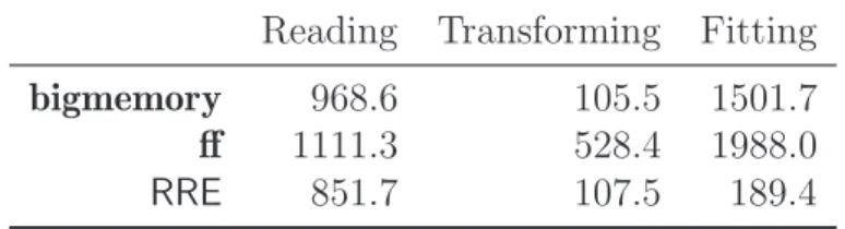
Table 2: Timing results (in seconds) for reading in the whole 12GB data, transforming to create new variables, and fitting the logistic regression with three methods: bigmemory, ff, and RRE.
Reading Transforming Fitting bigmemory 968.6 105.5 1501.7 ff 1111.3 528.4 1988.0
RRE 851.7 107.5 189.4
6
A Case Study
The airline on-time performance data from the 2009 ASA Data Expo (http://stat-computing.org/dataexp
is used as a case study to demonstrate a logistic model fitting with a massive dataset that exceeds the RAM of a single computer. The data is publicly available and has been used for demonstration with big data by Kane et al. (2013) and others. It con-sists of flight arrival and departure details for all commercial flights within the USA, from October 1987 to April 2008. About 12 million flights were recorded with 29 vari-ables. A compressed version of the pre-processed data set from the bigmemory project (http://data.jstatsoft.org/v55/i14/Airline.tar.bz2) is approximately 1.7GB, and it takes 12GB when uncompressed.
The response of the logistic regression is late arrival which was set to 1 if a flight was late by more than 15 minutes and 0 otherwise. Two binary covariates were created from the departure time: night (1 if departure occurred between 8pm and 5am) and weekend (1 if departure occurred on weekends and 0 otherwise). Two continuous covariates were included: departure hour (DepHour, range 0 to 24) and distance from origin to destination (in 1000 miles). In the raw data, the departure time was an integer of the HHmm format. It was converted to minutes first to prepare for DepHour. Three methods are considered in the case study: 1) combination of bigglm with package bigmemory; 2) combination of bigglm with package ff; and 3) the academic, single workstation version of RRE. The default settings of ff were used. Before fitting the logistic regression, the 12GB raw data needs to be read in from the csv format, and new variables needs to be generated. This leads to a total of 120,748,239 observations with no missing data. The R scripts for the three methods are in the supplementary materials for interested readers.
The R scripts were executed in batch mode on a 8-core machine running CenOS (a free Linux distribution functionally compatible with Red Hat Enterprise Linux which is officially supported byRRE), with Intel Core i7 2.93GHz CPU, and 16GB memory. Table 2 summarizes the timing results of reading in the whole 12GB data, transforming to create new variables, and fitting the logistic regression with the three methods. The chunk sizes were set to be 500,000 observations for all three methods. For RRE, this was set when reading in the data to theXDFformat; for the other two methods, this was set at the fitting stage using function bigglm. Under the current settings, RRE has a clear advantage in fitting with only 8% of the time used by the other two approaches. This is a result of the joint force of its using all 8 cores implicitly and efficient storage and retrieval of the
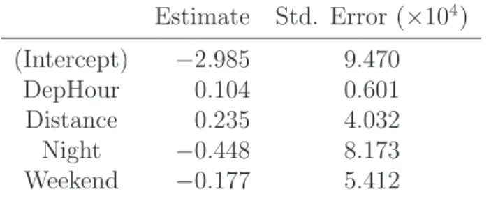
Table 3: Logistic regression results for late arrival. Estimate Std. Error (×104) (Intercept) −2.985 9.470 DepHour 0.104 0.601 Distance 0.235 4.032 Night −0.448 8.173 Weekend −0.177 5.412
Table 4: Time results (in seconds) for parallel computing quantiles of departure delay for each day of the week with 1 to 8 cores using foreach.
1 2 3 4 5 6 7 8
bigmemory 22.1 11.2 7.8 6.9 6.2 6.3 6.4 6.8 ff 21.4 11.0 7.1 6.7 5.8 5.9 6.1 6.8
data; the XDF version of the data is about 1/10 of the size of the external files saved by bigmemoryorff. Usingbigmemoryand usingff inbigglmhad very similar performance in fitting the logistic regression, but the former took less time in reading, and significantly less time (only about 1/5) in transforming variables of the latter. Thebigmemory method was quite close to the RRE method in the reading and the transforming tasks. The ff method took longer in reading and transforming than the bigmemory method, possibly because it used much less memory.
The results of the logistic regression are identical from all methods, and are summarized in Table 3. Flights with later departure hour or longer distance are more likely to be delayed. Night flights or weekend flights are less likely to be delayed. Given the huge sample size, all coefficients were highly significant. It is possible, however, that p-values can still be useful. A binary covariate with very low rate of event may still have an estimated coefficient with a not-so-low p-value (Schifano et al., 2015), an effect only estimable with big data.
As an illustration of foreach for embarrassingly parallel computing, the example in Kane et al. (2013) is expanded to include both bigmemory and ff. The task is to find three quantiles (0.5, 0.9, and 0.99) of departure delays for each day of the week; that is, 7 independent jobs can run on 7 cores separately. To make the task bigger, each job was set to run twice. The resulting 14 jobs were parallelized with foreach on the same Linux machine using 1 to 8 cores for the sake of illustration. The R script is included in the supplementary materials. The timing results are summarized in Table 4. There is little difference between the two implementations. When there is no communication overhead, with 14 jobs one would expect the run time to reduce to 1/2, 5/14, 4/14, 3/14, 3/14, 2/14, and 2/14, respectively, with 2, 3, 4, 5, 6, 7 and 8 cores. The impact of communication cost is obvious in Table 4. The time reduction is only closer to the expectation in the ideal case when the number of cores is smaller.
7
Discussion
This article presents a recent snapshot on statistical analysis with big data that exceed the memory and computing capacity of a single computer. Albeit under-appreciated by the general public or even mainstream academic community, computational statisticians have made respectable progress in extending standard statistical analysis to big data, with the most notable achievements in the open source R community. Packages bigmemory and ff make it possible in principle to implement any statistical analysis with their data structure. Nonetheless, for anything that has not been already implemented (e.g., survival analysis, generalized estimating equations, mixed effects model, etc.), one would need to implement an EMA version of the computation task, which may not be straightforward and may involve some steep learning curves. Hadoop allows easy extension of algorithms that do not require multiple passes of the data, but such analyses are mostly descriptive. An example is visualization, an important tool in exploratory analysis. With big data, the bottleneck is the number of pixels in the screen. The bin-summarize-smooth framework for visualization of large data of Wickham (2014a) with package bigvis(Wickham, 2013) may be adapted to work with Hadoop.
Big data present challenges much further beyond the territory of classic statistics, requir-ing joint workforce with domain knowledge, computrequir-ing skills, and statistical thinkrequir-ing (Yu, 2014). Statisticians have much to contribute to both the intellectual vitality and the prac-tical utility of big data, but will have to expand their comfort zone to engage high-impact, real world problems which are often less structured or with ambiguity (Jordan and Lin, 2014). Examples are to provide structure for poorly defined problems, or to develop meth-ods/models for new types of data such as image or network. As suggested by Yu (2014), to play a critical role in the arena of big data or own data science, statisticians need to work on real problems and relevant methodology and theory will follow naturally.
Acknowledgement
The authors thank Stephen Archut, Fang Chen, and Joseph Rickert for the big data analyt-ics information onSPSS,SAS, andRRE. An earlier version of the manuscript was presented at the “Statistical and Computational Theory and Methodology for Big Data Analysis” workshop in February, 2014, at the Banff International Research Station in Banff, AB, Canada. The discussions and comments from the workshop participants are gratefully acknowledged.
Supplementary Materials
Four R scripts (and their outputs), along with a descriptive README file are provided for the case study. The first three are the logistic regression with, respectively, combination of bigmemory with bigglm (bigmemory.R), combination of ff with bigglm (ff.R), and RRE
third one needsRRE. The fourth script is for the parallel computing withforeachcombined with bigmemory and ff, respectively.
References
Adler, D., Glser, C., Nenadic, O., Oehlschlgel, J., and Zucchini, W. (2014), ff: Memory-efficient Storage of Large Data on Disk and Fast Access Functions, r package version 2.2-13.
Andrieu, C. and Roberts, G. O. (2009), “The Pseudo-Marginal Approach for Efficient Monte Carlo Computations,” The Annals of Statistics, 697–725.
Bates, D., Francois, R., and Eddelbuettel, D. (2014), RcppEigen: Rcpp Integration for the Eigen Templated Linear Algebra Library, r package version 0.3.2.2.0.
Bickel, P. J., G¨otze, F., and van Zwet, W. R. (1997), “Resampling Fewer than n Observa-tions: Gains, Losses, and Remedies for Losses,” Statistica Sinica, 7, 1–31.
Blackford, L. S., Choi, J., Cleary, A., D’Azevedo, E., Demmel, J., Dhillon, I., Dongarra, J., Hammarling, S., Henry, G., Petitet, A., Stanley, K., Walker, D., and Whaley, R. C. (1997),ScaLAPACK Users’ Guide, Philadelphia, PA: Society for Industrial and Applied Mathematics.
Buckner, J., Seligman, M., and Wilson, J. (2013),gputools: A few GPU Enabled Functions, r package version 0.28.
Calderhead, B. (2014), “A General Construction for Parallelizing Metropolis–Hastings Al-gorithms,” Proceedings of the National Academy of Sciences, 111, 17408–17413.
Chambers, J. (2014), “Interfaces, Efficiency and Big Data,” 2014 UseR! International R User Conference.
Chapman, B., Jost, G., and Van Der Pas, R. (2008), Using OpenMP: Portable Shared Memory Parallel Programming, Cambridge, MA: MIT Press.
Chen, X. and Xie, M.-g. (2014), “A Split-and-Conquer Approach for Analysis of Extraor-dinarily Large Data,”Statistica Sinica, forthcoming.
Cohen, R. and Rodriguez, R. (2013), “High Performance Statistical Modeling,” Technical Report 401–2013, SAS Global Forum.
Cooper, N. (2014), bigpca: PCA, Transpose and Multicore Functionality for big.matrix Objects, r package version 1.0.
Dagum, L. and Enon, R. (1998), “OpenMP: An Industry Standard API for Shared-memory Programming,” Computational Science & Engineering, IEEE, 5, 46–55.
Davidian, M. (2013), “Aren’t We Data Science,” Amstat News, 433, 3–5. 22
de Villar, F. and Rubio, A. (2014),GUIProfiler: Profiler Graphical User Interface, r pack-age version 0.1.2.
Dean, J. and Ghemawat, S. (2008), “MapReduce: Simplified Data Processing on Large Clusters,” Commun. ACM, 51, 107–113.
Diebold, F. X. (2012), “A Personal Perspective on the Origin(s) and Development of “Big Data”: The Phenomenon, the Term, and the Discipline, Second Version,” Pier work-ing paper archive, Penn Institute for Economic Research, Department of Economics, University of Pennsylvania.
Eddelbuettel, D. (2013), Seamless R and C++ Integration with Rcpp, Springer.
— (2014), “CRAN Task View: High-performance and Parallel Computing with R,” Https://cran.r-project.org/web/views/HighPerformanceComputing.html.
Eddelbuettel, D. and Francois, R. (2014), RInside: C++ Classes to Embed R in C++ Applications, r package version 0.2.11.
Eddelbuettel, D., Fran¸cois, R., Allaire, J., Chambers, J., Bates, D., and Ushey, K. (2011), “Rcpp: Seamless R and C++ Integration,” Journal of Statistical Software, 40, 1–18. Eddelbuettel, D. and Sanderson, C. (2014), “RcppArmadillo: Accelerating R with
High-performance C++ Linear Algebra,” Computational Statistics and Data Analysis, 71, 1054–1063.
Efron, B. (1979), “Bootstrap Methods: Another Look at the Jackknife,” The annals of Statistics, 7, 1–26.
Emerson, J. W. and Kane, M. J. (2012), “Don’t Drown in the Data,”Significance, 9, 38–39. — (2013a), biganalytics: A Library of Utilities for big.matrix Objects of Package
bigmem-ory, r package version 1.1.1.
— (2013b), bigtabulate: table-, tapply-, and Split-like Functionality for Matrix and big.matrix Objects., r package version 1.1.2.
Enea, M. (2014), speedglm: Fitting Linear and Generalized Linear Models to Large Data Sets., r package version 0.2-1.0.
Fan, J., Han, F., and Liu, H. (2014), “Challenges of Big Data Analysis,” National Science Review, 1, 293–314.
Fan, J. and Lv, J. (2008), “Sure Independence Screening for Ultrahigh Dimensional Feature Space,” Journal of the Royal Statistical Society: Series B (Statistical Methodology), 70, 849–911.
— (2011), “Non-concace Penalized Likelihood with NP-dimensionality,”IEEE Transactions on Information Theory, 57, 5467–5484.