Optimal Top-k Generation of Attribute Combinations
based on Ranked Lists
Jiaheng Lu
†, Pierre Senellart
‡, Chunbin Lin
†, Xiaoyong Du
†, Shan Wang
†, and Xinxing Chen
†† School of Information and DEKE, MOE, Renmin University of China; Beijing, China
‡
Institut Télécom; Télécom ParisTech; CNRS LTCI; Paris, France
{jiahenglu, chunbinlin,duyong,swang,xxchen}@ruc.edu.cn, [email protected]
ABSTRACT
In this work, we study a novel top-kquery type, called top-k,m
queries. Suppose we are given a set of groups and each group con-tains a set of attributes, each of which is associated with a ranked list of tuples, with ID and score. All lists are ranked in decreasing order of the scores of tuples. We are interested in finding the best combi-nations of attributes, each combination involving one attribute from each group. More specifically, we want the top-kcombinations of at-tributes according to the corresponding top-mtuples with matching IDs. This problem has a wide range of applications from databases to search engines on traditional and non-traditional types of data (relational data, XML, text, etc.). We show that a straightforward extension of an optimal top-kalgorithm, the Threshold Algorithm (TA), has shortcomings in solving the top-k,mproblem, as it needs to compute a large number of intermediate results for each com-bination and reads more inputs than needed. To overcome this weakness, we provide here, for the first time, aprovably instance-optimalalgorithm and further develop optimizations for efficient query evaluation to reduce computational and memory costs and the number of accesses. We demonstrate experimentally the scalability and efficiency of our algorithms over three real applications.
Categories and Subject Descriptors
H.2.4 [Database Management]: Systems—Query processing; H.3.3 [Database Management]: Information Search and Retrieval—Search process
General Terms
Algorithms, Experimentation, Performance, Theory
Keywords
keyword search, package search, top-kquerying
1.
INTRODUCTION
During the last decade, the topic of top-kquery processing has been extensively explored in the database community due to its im-portance in a wide range of applications. In this work, we identify a
Permission to make digital or hard copies of all or part of this work for personal or classroom use is granted without fee provided that copies are not made or distributed for profit or commercial advantage and that copies bear this notice and the full citation on the first page. To copy otherwise, to republish, to post on servers or to redistribute to lists, requires prior specific permission and/or a fee.
SIGMOD ’12,May 20–24, 2012, Scottsdale, Arizona, USA. Copyright 2012 ACM 978-1-4503-1247-9/12/05 ...$10.00.
novel top-kquery type that has wide applications and requires novel algorithms for efficient processing. Before we give the definition of our problem, we describe an interesting example to motivate it.
Assume a basketball coach plans to build a good team for an important game (e.g., Olympic games). He would like to select a combination of athletes including forward, center, andguard
positions, by considering their historical performance in games. See Figure 1 for the example data, which comes from the NBA 2010– 2011 pre-season. Each tuple in Figure 1(a) is associated with a pair (game ID,score), where thescoreis computed by an aggregation of various scoring items provided by the NBA for this game. To build a good team, one option is to select athletes with the highest score in each group (e.g., “Juwan Howard” in the “forward” group), or to calculate the average scores of athletes across all games. However, both methods overlook an important fact: a strong team spirit is critical to the overall performance of a team. Therefore a better way is to evaluate the performance of athletes by considering their combined scores in thesamegame. We can formalize this problem as to select the top-kcombinations of athletes according to their best top-maggregate scores for gameswhere they played together. For example, as illustrated in Figure 1,F2C1G1is the best combination
of athletes, as the top-2 games in which the three athletes played together areG02 andG05, and 40.27 (= 21.51+18.76) is the highest overall score (w.r.t. the sum of the top-2 scores) among all eight combinations. We study in this paper a new query type called top-k,mquery that captures this need of selecting the top combinations of different attributes, when each attribute is described by a ranked list of tuples.
1.1
Problem description
Given a set of groupsG1,. . . ,Gn where each groupGicontains
multiple attributesei1,. . . ,eili, we are interested in returning top-k
combinations of attributes selected from each group. As an example, recall Figure 1: there are three groups, i.e.,forward,center, and
guard, and one athlete corresponds to one attribute in each group. Our goal is to select a combination of three athletes, each from a different group.
We suppose that each attributeeis associated with a ranked listLe,
where each tupleτ∈ Leis composed of an IDρ(τ) (taken out of
an arbitrary set of identifier) and a scoreσ(τ) (from an arbitrary fully ordered set, say, the reals). The list is ranked in descending order of the scores. In the example NBA data, each athlete has a list containing the game ID and the corresponding score. Given a combinationof attributes, amatch instanceIofis a set of tuples based on some arbitrary join condition on tuple IDsρ(τ) from lists. For example, the gameG02 (including the three tuples (G02, 8.91), (G02, 6.01), (G02, 6.59)) is a match instance by the equi-join of the game IDs. In the top-k,mproblem, we are interested in returning top-kcombinations of attributes which have the highest
Center
Forward Guard
F1 F2 C1 C2 G1 G2
Juwan Howard LeBron James Chris Bosh Eddy Curry Dwyane Wade Terrel Harris (G02, 8.91) (G08, 8.07) (G05, 7.54) (G10, 7.52) (G03, 6.14) (G01, 5.05) (G04, 5.01) (G09, 3.34) ĂĂ (G06, 3.01) (G01, 3.81) (G06, 3.59) (G04, 3.21) (G07, 3.03) (G09, 2.07) (G11, 1.70) (G10, 1.62) (G02, 1.59) ĂĂ (G08, 1.19) (G02, 6.59) (G03, 6.19) (G04, 5.81) (G05, 4.01) (G01, 3.38) (G09, 2.25) (G06, 1.52) (G08, 1.51) ĂĂ (G07, 1.00) (G09, 7.10) (G03, 6.01) (G04, 3.79) (G08, 3.02) (G05, 2.89) (G02, 2.52) (G01, 2.00) (G10, 1.59) ĂĂ (G06, 1.52)
(a) Source data of three groups
(b) Top-2 aggregate scores for each combination
40.27(=21.51+18.76) is the largest among the aggregate scores of top-2
(G01, 9.31) (G07, 9.02) (G03, 8.87) (G04, 5.02) (G11, 4.81) (G08, 4.02) (G06, 4.31) (G05, 3.59) ĂĂ (G09, 2.06) (G05, 7.21) (G02, 6.01) (G06, 5.58) (G10, 5.51) (G04, 5.00) (G11, 3.09) (G01, 2.06) (G08, 2.03) ĂĂ (G09, 1.98) F1C1G1 (G04, 15.83) (G05, 14.81) F1C1G2 F1C2G1 F1C2G2 F2C1G1 F2C1G2 F2C2G1 F2C2G2 (G04, 13.81) (G05, 13.69) (G01, 16.50) (G04, 14.04) (G01, 15.12) (G07, 12.05) (G02, 21.51) (G05, 18.76) (G05, 17.64) (G02, 17.44) (G02, 17.09) (G04, 14.03) (G02, 13.02) (G09, 12.51)
…
…
…
…
…
…
…
…
Figure 1: Motivating example using 2010–2011 NBA data. Our purpose is to select one athlete from each of the three groups. The best combination isF2C1G1. Values in bold font indicate tuples contributing to the score of this best combination.
overall scores over their top-mmatch instances by a monotonic aggregate function. Suppose thatk=1,m=2, and that scores are aggregated using the sum function. The top-2 match instances of
F2C1G1areG02 andG05 and their overall score is 40.27, which
is the highest overall score among the top-2 match instances of all combinations. Therefore, we say that the answer of the top-1,2 query for the problem instance in Figure 1 is the combinationF2C1G1.
1.2
Applications
Next we give more use-case scenarios of top-k,mqueries, which shed some light on the generality and importance of top-k,mmodels in practice.
Use-case 1.
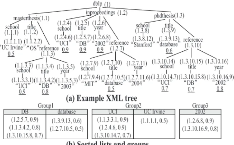
Top-k,mqueries are useful inXML databases. Asimple yet effective way to search an XML database is keyword search. But in a real application it is often the case that a user issues a keyword queryQwhich does not return the desired answers due to the mismatch between terms in the query and in documents. A com-mon strategy for remedying this is to perform some query rewriting, replacing query terms with synonyms that provide better matches. Interestingly, top-k,mqueries find an application in this scenario. Specifically, for each keyword (or phrase)qinQ, we generate a groupG(q) that contains the alternative terms ofqaccording to a dictionary which containssynonymsandabbreviationsofq. For ex-ample, given a queryQ=hDB,UC Irvine,2002i, we can generate three groups:G1 ={“DB”,“database”},G2 ={“UCI”,“UC Irvine”},
andG3={“2002”}. We assume that each term inG(q) is associated
with a list of node identifiers (e.g., JDewey IDs [7]) and scores (e.g., information-retrieval scores such as tf-idf [4]). See Figure 2 for an example XML tree and scores. The goal of top-k,mqueries is to find the top-kcombinations (of terms) by considering the corresponding top-msearch results in the XML database. Therefore, a salient fea-ture of the top-k,mmodel for the refinement of XML keyword query is that it guarantees that the suggested alternative queries have high quality results in the database within the top-manswers.
Use-case 2.
Top-k,mqueries also have applications inevidencecombination miningin medical databases [2]. The goal is to predict or screen for a disease by mining evidence combination from clinical and pathological data. In a clinical database, each evidence refers
dblp inproceedings school (1.1.1) (1.1.1.1) ĀUC Irvineā masterthesis(1.1) phdthesis(1.3) school ĀUCIā (1.3.10.14) (1.3.10.14.7) Ādatabaseāreference title (1.3.10) (1.3.8) (1.3.8.12) (1) title ĀOSā (1.1.2) (1.1.2.2) DB
(a) Example XML tree
(b) Sorted lists and groups
0.5 0.7 title (1.3.10.15) year Ā2002ā (1.3.10.16.9) (1.3.10.15.8) (1.3.10.16) 0.7 ĀDBā school ĀUCIā (1.2.4) (1.2.4.6) (1.2) 0.9 title (1.2.5) year Ā(1.2.6.8)2002ā (1.2.5.7) (1.2.6) 0.9 ĀDBā 0.9 0.8 Group1 database (1.2.5.7, 0.9) (1.1.3.4.2, 0.8) (1.3.10.15.8, 0.7) (1.3.9.13, 0.6) (1.2.7.10.5, 0.5) Group2 2002 Group3 UCI UC Irvine (1.1.3.3.1, 0.9) (1.2.4.6, 0.9) (1.3.10.14.7, 0.7) (1.1.1.1, 0.5) (1.2.6.8, 0.9) (1.3.10.16.9, 0.8) school ĀUCIā (1.1.3.3) (1.1.3.3.1) reference (1.1.3) 0.9 title (1.1.3.4) year Ā2003ā (1.1.3.5.3) (1.1.3.4.2) (1.1.3.5) 0.8 ĀDBā ĀStanfordā school (1.3.9) (1.3.9.13) 0.6 reference (1.2.7.9) (1.2.7) title (1.2.7.10) year Ā2004ā (1.2.7.11.6) (1.2.7.10.5) (1.2.7.11) 0.5 Ādatabaseā (1.2.7.9.4) ĀMITā schoolFigure 2: An example illustrating XML query refinement using the top-k,m framework. The original query Q =
hDB,UC Irvine,2002i is refined into hDB,UCI,2002i. Each
term is associated with an inverted list with the IDs and weights of elements. Underlined numbers in the XML tree denote term scores.
to a group and different degrees of the evidence act as different attributes. For examplequeasiness,headaches,vomit, anddiarrhea
are four pieces of evidence (referring to groups) foracute enteritis, and each evidence has different degrees (referring to attributes), e.g.,
very low,low,middle,high,very high. Each tuple in a list associated to an attribute consists of the patient ID and the probability the patient catches the disease. The goal of the top-k,mquery is to find the top-kcombinations of different degrees of evidences ordered by the aggregate values of the probabilities of top-mpatients for which there is the highest belief this disease is involved.
Use-case 3.
Top-k,mqueries may finally have applications inpackage recommendation systems, e.g., thetrip selectionproblem. Consider a tourist who is interested in planing a trip by choosing one hotel, one shopping mall, and one restaurant in a city. Assume that we have survey data provided by users who made trips be-fore. The data include three groups and each group have multiple attributes (i.e., names of hotels, malls, or restaurants), each of which is associated with a list of users’ IDs and grades. Top-k,mqueries recommend top-ktrips which are combinations of hotels, malls, and restaurants based on the aggregate value of the highestmscores of the users who had the experience of this exact trip combination.
Generally speaking, top-k,mqueries are of use in any context where one is interested in obtaining combinations of attributes asso-ciated with ranked lists. In addition, note that the model of top-k,m
queries offers great flexibility in problem definitions to meet the various requirements that applications may have, in particular in the adjustment of themparameter. For example, in the application to XML keyword search, a user is often interested in browsing only the top few results, say 10, which means we can setm=10 to guarantee the search quality of the refined keywords. In another application, e.g., trip recommendation, if a tourist wants to consider the average score of all users, then we can definemto be large enough to take the scores of all users into accounts. (Of course, in this case, the number of accesses and the computational cost are higher.)
1.3
Novelty and contributions
The literature on top-kquery processing in relational and XML databases is particularly rich [5–8, 12, 13]. We stress the essential
difference between top-kqueries (e.g., as in [8]) and our top-k,m
problem: the latter returns the top-k combinationsof attributes in groups, but the former returns the top-k tuples(objects). Therefore, a top-k,mproblem cannot be reduced to a top-kproblem through a careful choice of the aggregate function. In addition, contrarily to the top-kproblem, we argue that top-k,mqueries cannot be transformed into a SQL (nested) query, since SQL queries return tuples but our goal is to returnattribute combinationsbased on ranked inverted lists, which is not something that the SQL language permits. To the best of our knowledge, this is the first top-kwork focusing on selecting and ranking sets of attributes based on ranked lists, which is a highly non-trivial extension of the traditional top-kproblem. An extended discussion about the difference between top-k,mqueries and the existing top-kqueries can be found in Section 3.
To answer a top-k,mquery, one method, called extended TA (for short ETA hereafter), is to compute all top-mresults for each combination by the well-known threshold algorithm (TA) [8] and then to pick the top-kcombinations. However, this method has one obvious shortcoming: it needs to compute top-mresults for
eachcombination and readsmoreinputs than needed. To address this problem, we develop a set ofprovably optimalalgorithms to efficiently answer top-k,mqueries.
Following the model of TA [8], we allow both random access and sorted access on lists. Sorted accesses mean to perform sequential scan of lists and random access can be performed only on objects which are previously accessed by sorted access. For example, con-sider Figure 1 again. When the first tuple (G05,7.21) ofC1is read,
the random access enables us to quickly locate all tuples whose ID areG05 (e.g., (G05,7.54) inF2). We propose an algorithm called
ULA (Upper and Lower boundsAlgorithm) to avoid the needs to compute top-mresults of combinations (Section 4) and thus to significantly reduce the computation costs compared to ETA.
We then bring to light some key observations and develop an optimized algorithm called ULA+, which minimizes the number of accesses and consequently reduces the computational and memory costs. The ULA algorithm needs to compute bounds (lower and upper bounds) for each combination, which may be expensive when the number of combination is large. In ULA+, we avoid the need to compute bounds for some combinations by carefully designing the conditions to prune away useless combinations without reading any tuple in the associated lists. We also propose a native structure calledKMG graphto avoid the useless sorted and random accesses in lists to save computational and memory costs.
We study the optimal properties of our algorithms with the notion ofinstance optimality[8] that reflects how well a given algorithm performs compared to all other possible algorithms in its class. We show that two properties dictate the optimality of top-k,m al-gorithms in this setting: including (1) the number of attributes in groupGi, namely|Gi|, which is part of the input of the problem; and
(2) whether wild guesses are allowed. Following [8], wild guesses mean random access to objects which have not been seen by sorted access. Only if each|Gi|is treated as a constant and there are no
wild guesses is our algorithm guaranteed to beinstance-optimal. In addition, we show that the optimality ratio of our algorithms is tight in a theoretical sense. Unfortunately, if either|Gi|is considered
variable or wild guesses exist (uncommon cases in practice), our algorithms are not optimal. But we show that in these casesno
instance-optimal algorithm exists.
To demonstrate the applicability of the top-k,mframework, we apply it to the problem of XML keyword refinement. We show how to judiciously design the aggregation functions and join predicates to reflect the semantic of XML keyword search. We then adapt the three algorithms: ETA, ULA and ULA+(from the most
straight-forward to the highly optimized one) to efficiently answer an XML top-k,mproblem (Section 5).
We verify the efficiency and scalability of our algorithms using three real-life datasets (Section 6), including NBA data, YQL trip-selection data, and XML data. We find that our top-k,malgorithms result in order-of-magnitude performance improvements when com-pared to solutions based on the baseline algorithm. We also show that our XML top-k,mapproach is a promising and efficient method for XML keyword refinement in practice.
To sum up, this article presents a new problem with important applications, and a family of provably optimal algorithms. Compre-hensive experiments verify the efficiency of solutions on three real datasets.
2.
PROBLEM FORMULATION
Given a set of groupsG1,. . . ,Gn where each groupGicontains
multiple attributesei1,. . . ,eili, we suppose that each attributeeis
associated with a ranked listLe, where each tupleτ∈Leis composed
of an IDρ(τ) and a scoreσ(τ). The list is ranked by the scores in descending order. Let = (e1i, . . . ,en j)∈ G1× · · · ×Gn denote
an element of the cross-product of thengroups, hereafter called
combination. For instance, recall Figure 1, every three athletes from different groups form a combination (e.g., {Lebron James,Chris Bosh,Dwyane Wade}).
Given a combination, a match instanceI is defined as a set of tuples based on some arbitrary join condition on IDs of tuples from lists. Each tuple in a match instance should come from different groups. For example, in Figure 1, given a com-bination {Juwan Howard, Eddy Curry, Dwyane Wade}, then
{(G01,9.31),(G01,3.81),(G01,3.38)}is a match instance for the gameG01. Furthermore, we define two aggregate scores:tScoreand
cScore: the score of each match instanceIis calculated bytScore, and the top-mmatch instances are aggregated to obtain the overall score, calledcScore. More precisely, given a match instanceI
defined on,
tScore(I)=F1(σ(τ1), . . . , σ(τn))
whereF1is a function: Rn→Randτ1, . . . , τn form the matching
instanceI. Further, given an integermand a combination,
cScore(,m)= max I 1,...,Im distinct {F2(tScore(I1), . . . ,tScore(I m))} whereF2is a functionRm→ RandI1,. . . ,I
mare anymdistinct
match instances defined on the combination. Intuitively,cScore
returns the maximum aggregate scores ofmmatch instances. Fol-lowing common practice [8], we require bothF1andF2functions to be monotonic, i.e., the greater the individual score, the greater the aggregate score. This assumption captures most practical scenarios, e.g., if one athlete has a higher score (and the other scores remain the same), then the whole team is better.
Definition1 (top-k,mproblem). Given groupsG1, . . . ,Gn, two
integersk,m, and two score functionsF1,F2, thetop-k,m problem
is an (n+4)-tuple (G1, . . . ,Gn,k,m,F1,F2). A solution is an
or-dered setScontaining the top-kcombinations=(e1i, . . . ,en j)∈ G1× · · · ×Gnordered bycScore(,m).
Example 2. Consider a top-1,2 query on Figure 1, and assume
thatF1 andF2 aresum. The final answerSis {F2C1G1}. This
is because the top-1 match instanceI1 ofF2C1G1 consists of
tu-ples (G02,8.91), (G02,6.01) and (G02,6.59) of the gameG02 withtScore21.51=8.91+6.01+6.59. And the second top in-stanceI2 consists of tuples whose game ID isG05 withtScore
18.76=7.54+7.21+4.01. Therefore, thecScoreofF2C1G1is
40.27=21.51+18.76, which is the highest score among all combi-nations.
3.
BACKGROUND AND RELATED WORK
Before we describe the novel algorithms for top-k,mqueries, we pause to review some related works about top-kqueries. Top-k
queries were studied extensively for relational and XML data [5–8, 12, 13, 22]. Notably, Fagin, Lotem, and Naor [8] present a compre-hensive study of various methods for top-kaggregation of ranked inputs. They identify two types of accesses to the ranked lists: sorted accesses and random accesses. In some applications, both sorted and random accesses are possible, whereas, in others, some of the sources may allow only sorted or random accesses. For the case where both sorted and random accesses are possible, a threshold algorithm (TA) (independently proposed in [10, 20]) retrieves ob-jects from the ranked inputs in a round-robin fashion and directly computes their aggregate scores by using random accesses to the lists where the object has not been seen. Fagin et al. prove that TA is an instance-optimal algorithm. In this paper, we follow the line of TA to support bothsortedaccesses andrandomaccesses for efficient evaluation of top-k,mquery. We prove that our algorithm is also an instance-optimal algorithm and its optimality ratio is tight.
There is also a rich literature for top-kqueries in other envi-ronments, such as no random access [9, 18], no sorted access on restricted lists [5, 6], no need for exact aggregate score [11], or ad-hoc top-kqueries [15, 23]. For example, Mamoulis, Yiu, Cheng and Cheung [18] proposed a family of optimizations for top-kqueries in the case ofno random accesses. They impose two phases (growing
andshrinking) that any top-kalgorithm should go through, and per-form optimizations on theshrinkingphase to reduce the number of accesses. Theobald, Schenkel and Weikum [21] proposed a top-k
query processor for efficient and self-tuning query expansion, which is related to the XML keyword refinement method described in Section 5. In contrast to our work, Theobald et al. also support a non-fixed number of keywords in the refined query; however, no op-timality guarantees are given. Recently, Jin and Patel [13] proposed a novel sequential access scheme for top-kquery evaluation, which outperforms existing schemes. For more information about top-k
query evaluation, readers may refer to an excellent survey [12] by Ilyas, Beskales, and Soliman.
In this article, we argue that top-k,mqueries are new types of queries and that the existing top-kalgorithms cannot be used to solve them. For example, consider the ad-hoc top-kqueries in [15, 23]. Note the difference regarding the notion of “group” between those works and ours. For ad-hoc queries, a group refers to a set of objects (rows) which satisfy certain predicates, while a group in this article means a set of attributes (columns). Therefore, top-k,mqueries, in a different approach from ad-hoc top-kqueries, focus on the ranking of the combinations of attributes (notobjects). To the best of our knowledge, this is the first work focusing on selecting and ranking the set of attributes, which is a highly non-trivial extension of the traditional top-kproblem.
Top-kprocessing in XML databases has recently gained more at-tention since XML has become the preferred medium for formatting and exchanging data in many domains [1, 7, 19]. There are various types of problems on XML top-kprocessing, including top-ktwig query processing [1, 19], top-kkeyword search [4], top-k probabilis-tic query processing [16] and top-kkeyword cleansing [17]. In this article, we demonstrate how to apply the framework of top-k,mon the problem of XML top-kkeyword refinement. Note the diff er-ence between keyword cleansing [17] and keyword refinement: the former rewrites the query by fixing spelling errors, but the latter
rewrites the query using semantic knowledge such as synonyms and abbreviations. Both approaches are complementary in query pro-cessing and can be used together to improve search engine results.
4.
TOP-K,M ALGORITHMS
In this section we begin our study of an efficient top-k,malgorithm which can stop earlier than the straightforward algorithm (i.e., ETA mentioned earlier), by avoiding the need to compute the exact top-m
scores for each combination. We propose a family of optimizations to improve the performance by reducing the number of accesses and computational and memory costs. We also analyze the optimality properties for proposed algorithms.
4.1
Access model: sorted and random accesses
As mentioned in the Introduction, given an instance of a top-k,m
problem, following the practice in the top-kliterature (e.g., [8]), we support both sorted and random access. Sorted accesses read the tuple of lists sequentially and random accesses quickly locate tuples whose ID has been seen by sorted access (assuming the existence of an index to achieve this goal). For example, in Figure 1, at depth 1 (depthdmeans the number of tuples seen under sorted access to a list isd), consider the combination “F2C1G1”; the tuples seen by
sorted access are (G02,8.91), (G05,7.21), (G02,6.59) and we can quickly locate all tuples (i.e., (G02,6.01), (G05,7.54), (G05,4.01)) whose IDs areG02 orG05 by random accesses.
4.2
Baseline algorithm: ETA
To answer a top-k,mquery, one straightforward method (called extended TA, or ETA for short) is to first compute all top-mresults for each combination by the well-known threshold algorithm TA [8] and then pick the top-kcombinations. However, this method has one obvious shortcoming: it needs to compute top-mresults for
eachcombination and readsmoreinputs than needed. For example, in Figure 1, ETA needs to compute the top-2 scores for all eight combinations (see Figure 1(b)). Indeed, this method isnot instance-optimalin this context. To address this problem, we develop a set of
provably optimalalgorithms to efficiently answer top-k,mqueries.
4.3
Top-k,m algorithm: ULA
When designing an efficient top-k,malgorithm, informally, we observe that a combinationcannot contribute to the final answer if
there exist k distinct combinations whose lower bounds are greater than the upper bounds of. To understand this, consider the top-1,2 query in Figure 1 again. At depth 1, for the combination “F2C1G1”,
we get two match instancesG02 andG05 through the sorted and random accesses. Then the lower bound of the aggregate score (i.e.,cScore) of “F2C1G1” is at least 40.27 (i.e., (7.54+7.21+
4.01)+(8.91+6.01+6.59)). At this point, we can claim that some combinations are not part of answers. This is the case of “F2C2G1”,
whosecScoreis no more than 38.62 (=2×(8.91+3.81+6.59)). Since 38.62 < 40.27,F2C2G1 cannot be the top-1 combination.
We next formalize this observation by carefully defining lower and upper bounds of combinations. We start by presenting threshold values, which will be used to estimate the upper bounds for the unseen match instances.
Definition3 (threshold value). Let=(e1i, . . . ,en j)∈G1×
· · · ×Gnbe an arbitrary combination, andτithe current tuple seen
under sorted access in listLi. We define thethreshold valueTof
the combinationto beF1(σ(τ1), . . . , σ(τn)), which is the upper
bound oftScorefor any unseen match instance of.
As an example, in Figure 1(a), consider the combination = “F2C1G1”, at depth 1. The current tuples are (G02,8.91), (G05,7.21),
(G02,6.59). Assume F1 = sum, we have for threshold value
T=8.91+7.21+6.59=22.71.
Definition4 (lower bound). Assume one combinationhas
seenm0
distinct match instances. Then thelower boundof the
cScoreofis computed as follows:
min= F2(tScore(I1), . . . ,tScore(I m0),0, . . . ,0 | {z } m−m0 ) m0<m
max{F2(tScore(Ii), . . . ,tScore(I
j) | {z } m )} m0 >m Whenm0<
m, we use the minimal score (i.e., zero) of unseen
m−m0
match instances to estimate the lower bound of thecScore. On the other hand, whenm0
>m,minequals the maximal aggregate
scores ofmmatch instances.
Definition5 (upper bound). Assume one combination has
seenm0
distinct match instances, where there arem00
match instances (m00
6m0
) whose scores aregreater than or equal toT. Then the
upper boundof thecScoreofis computed as follows:
max= F2(tScore(I1), . . . ,tS core(I m00),T , . . . , T | {z } m−m00 ) m00<m
max{F2(tScore(Ii), . . . ,tScore(I
j) | {z } m )} m00 >m Ifm00 <
m, it means that there is still a chance that we will see a new match instance whosetScorecontributes to the final
cScore. Therefore, the computation ofmaxshould be padded with
m−m00
copies of the threshold value (i.e.,T), which is the upper bound oftScorefor all unseen match instances. Otherwise,m00
> m, meaning that the final top-mresults are already seen and thus
max=cScore(,m) now.
Example 6. This example illustrates the computation of the
up-per and lower bounds. See Figure 1 again. Assume thatF1 and
F2aresum, and the query is top-1,2. At depth 1, the combination
“F2C1G1” read tuples (G02,8.91), (G05,7.21), and (G02,6.59) by
sorted accesses, and (G05,7.54), (G02,6.01), (G05,4.01) by ran-dom accesses.m0=
m=2. Therefore, the current lower bound of “F2C1G1” is 40.27 (i.e., (7.54+7.21+4.01)+(8.91+6.01+6.59)=
18.76+21.51), since the two match instances ofF2C1G1areG02
andG05. The thresholdTF2C1G1=8.91+7.21+6.59=22.71 and
m00 =
0, since 18.76<22.71 and 21.51<22.71. Therefore, the upper bound is 45.42 (i.e., 22.71+22.71). In fact, the finalcScore
of “F2C1G1” is exactly 40.27 which equals the current lower bound.
Note that the values of lower and upper bounds are dependent of the depth where we are accessing. For example, at depth 2, the upper bound of “F2C1G1” decreases to 41.78 (i.e., 21.51+20.27) and the
lower bound remains the same.
The following lemmas show how to use the bounds above to determine if a combinationcan be pruned safely or confirmed to be an answer.
Lemma7 (drop-condition). One combinationdoes not
con-tribute to the final answers if there are k distinct combinations 1,. . . ,ksuch thatmax<min{imin|16i6k}.
Proof. The aggregate score of the top-mmatch instances is no
more then the upper bound of, i.e.,cScore(,m)6max. And∀i∈
[1,k],cScore(i,m)>imin, since the min
i is the lower bound ofi.
Therefore,cScore(,m)<min{cScore(0
i,m)| |16i6k}, which
means thatcannot be one of the top-kanswers, as desired. Lemma8 (hit-condition). One combinationshould be an
an-swer if there are at least Ncom−k (Ncom is the total number of
the combinations) distinct combinations1,. . . ,Ncom−k, such that
min
>max{max
i |16i6Ncom−k}.
Proof. The aggregate score of the top-mmatch instances ofis
no less than the lower bound of, i.e.,cScore(,m)>min. And
∀i∈[1,Ncom−k], maxi >cScore(i,m). Therefore,cScore(,m)>
max{cScore(i,m) | 1 6 i 6 Ncom−k}, meaning that the top-m
aggregate score ofis larger than or equal to that of otherNcom−k
combinations. Thereforemust be one of the top-k,manswers. Definition9 (termination). A combinationcan beterminated
ifmeets one of the following conditions: (i) the drop-condition, (ii) the hit-condition, or (iii)has seenmmatch instances whose
tScores are greater than or equals to the threshold valueT. Intuitively, one combination is terminated if we do not need to compute its lower or upper bounds any further. The first two conditions in the above definition are easy to understand. The third condition means that we have found top-mmatch instances of. Note that we may not see the final top-mmatch instances when satisfy the drop- or hit-condition.
We are now ready to present a novel algorithm namedULA
(Upper andLower boundsAlgorithm), that relies on the dynamic computing of upper and lower bounds of combinations (see Algo-rithm 1).
Algorithm 1The ULA algorithm
Input: a top-k,mproblem instance withngroupsG1, . . . ,Gn, where
each group has multiple listsLi j∈Gi.
Output: top-kcombinations of attributes in groups.
(i) Do sorted access in parallel to each of the sorted listsLi j. As
a tupleτis seen under sorted access in some list, do random access to all other lists inGj(j,i) to find all tuplesτ0such
thatρ(τ)=ρ(τ0
).
(ii) For each unterminated combination(by Definition 9), com-puteminandmax, and check ifcan be terminated now.
(iii) If there are at least k combinations which meet the hit-condition, then the algorithm halts. Otherwise, go to step (i). (iv) LetYbe a set containing thekcombinations (breaking ties
arbitrarily) when ULA halts. OutputY.
In the last step of the algorithm, note that the setYis unordered by
cScore. In the case where the output set should be ordered bycScore, we need to continuously maintain the lower and upper bounds of objects inYuntil their order is clear.
Example 10. We continue the example of Figure 1 to illustrate
the ULA algorithm. First, in step (i) (at depth 1), ULA performs sorted accesses on one row for each list and does the correspond-ing random accesses. In step (ii) (at depth 1 again), it computes the lower and upper bounds for each combination, and then three combinationsF1C2G2,F2C2G1andF2C2G2are safely terminated,
since their upper bounds (i.e.,max
F1C2G1 = 39.42, max
F2C2G1 = 38.62
andmax
F2C2G2 = 39.64) are less than the lower bound of F2C1G1
(min
F2C1G1=40.27). Next, we go to step (i) again (at depth 2), as there
is no combination satisfying the hit-condition in step (iii). Finally, at depth 4,F2C1G1meets the hit-condition and the ULA algorithm
halts. To understand the advantage of ULA over ETA, note that ETA cannot stop at depth 4, sinceF2C2G1does not yet obtain its top-2
match instances. Indeed, ETA stops at depth 5 with 54 accesses, whereas ULA performs only 50 accesses by depth 4.
4.4
Optimized top-k,m algorithm: ULA+
In this subsection, we present several optimizations to minimize the number of accesses, memory cost, and computational cost of the ULA algorithm by proposing an extension, called ULA+.
Pruning combinations without computing the bounds.
The ULA algorithm has to compute the lower and upper bounds for each combination, which may be an expensive operation when the number of combinations is large. We next propose an approach which prunes away many useless combinations safelywithout com-puting their upper or lower bounds.
We sort all lists in the same group by the scores of their top tuples. Notice that all lists are sorted by decreasing order. Intuitively, the combinations with lists containing small top tuples are guaranteed not to be part of answers, as their scores are too small. Therefore, we do not need to take time to compute their accurate upper and lower bounds. We exploit this intuitive observation by defining the precise condition under which a combination can be safely pruned without computing its bounds. We first define a relationship between two combinations calleddominating.
Given a groupGin a top-k,mproblem instance, letLeandLtbe
two lists associated with attributese,t∈G, we sayLedominates Lt, denotedLeLtifLe.σ(τm)>Lt.σ(τ1), whereτidenote theith
tuple in the list. That is, the score of themthtuple inLeis greater
than or equal to the score of thefirsttuple inLt.
Definition11 (domination). A combination={e1, . . . ,en} is
said todominate another combinationξ ={t1, . . . ,tn} (denoted
ξ) if for every 1>k>n, eitherei=tiorLeiLtiholds, where eiandtiare two (possibly identical) attributes of the same groupGi.
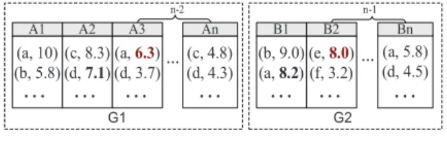
For example, in Figure 3, there are two groupsG1andG2. We
say that the combination “A2B1” dominates “A3B2”, because in the
groupG1, 7.1>6.3 and inG2, 8.2>8.0. In fact, “A2B1” dominates
all combinations of attributes fromA3toAninG1and fromB2toBn
inG2. Note that the lists in each group here are sorted by the scores
of the top tuples.
Lemma 12. Given two combinationsandξ, ifdominatesξ
then the upper bound ofis greater than or equal to that ofξ.
Proof. Ifdominatesξ, then for every attributeeinξ, ife<,
then there is an attributetin, s.t. the m-th tuple in the listLe
has a larger score than the first tuple in Lt. Therefore, the
up-per bound ofmmatch instances of is greater than or equal to that ofξ. More formally, ξ⇒ ∀i,Lei.σ(τm) > Lti.σ(τ1)⇒ F1(Le1.σ(τm),. . ., Len.σ(τm)) >F1(Lt1.σ(τ1),. . ., Ltn.σ(τ1)), since
F1 is monotonic. Som×(F1(Le1.σ(τm), . . . ,Len.σ(τm))) > m×
(F1(Lt1.σ(τ1), . . . ,Ltn.σ(τ1))). Note that max
>m×(F1(Le1.σ(τm), . . . ,Len.σ(τm))),
since the threshold value and the scores of the unseen match in-stances ofare no less thanF1(Le1.σ(τm), . . . ,Len.σ(τm)). In
addi-tion, it is easy to verify thatξmax
6m×(F1(Lt1.σ(τ1), . . . ,Ltn.σ(τ1))).
Therefore,max
>ξmaxholds, as desired.
According to Lemma 12, ifmeets the drop-condition (Lemma 7), it means the upper bound of is small, then any combinationξ which is dominated by(i.e.,ξ’s upper bound is even smaller) can be pruned safely and quickly.
To apply Lemma 12 in our algorithm, the lists are sorted in de-scending order by the score of the first tuple in each list, which can be done off-line. We first accessmtuples sequentially for each list and perform random accesses to obtain the corresponding match instances. Then we consider two phases. (i)Seed combination selection. As the name indicates, seed combinations are used to trigger the deletion of other useless combinations. We pick the lists in descending order, and construct the combinations to compute their upper and lower bounds until we find one combinationwhich meets the drop-condition, thenis selected as the seed combination.
(a, 10) (b, 5.8) (c, 8.3) (d, 7.1) (a, 6.3) (d, 3.7) (b, 9.0) (a, 8.2) Ă (e, 8.0) (f, 3.2) (c, 4.8) (d, 4.3) (a, 5.8) (d, 4.5) Ă A1 A2 A3 An B1 B2 Bn n-2 n-1 G1 G2
…
…
…
…
…
…
…
Figure 3: An example for Lemma 12
(ii)Dropping useless combinations. By Lemma 12, all combinations which are dominated byare also guaranteednotto contribute to final answers. For each groupGi, assuming that the seed
combina-tioncontains the listLaiinGi, then we find all listsLbisuch that LaiLbi. This step can be done efficiently as all lists are sorted by
their scores of first tuples. Therefore, all the combinations which are constructed fromLbican be dropped safely without computing
their upper or lower bounds.
Example 13. See Figure 3. Assume the query is top-1,2 and
F1=F2=sum. The lists are sorted in descending order according
to the score of the first tuple. We access the lists in descending order to find the seed combination, which isξ=(A2,B1) (ξmax=2×(7.1+
8.2)=30.6< min,={A
1,B1}). InG1,∀i∈[3,n]LA2LAi(e.g., LA2LA3, since 7.1>6.3). Similarly, inG2,∀i∈[2,n]LB1LBi.
Therefore all combinations (Ai,Bj) (∀i∈[3,n],j∈[2,n]), as well as
(A2,Bj) and (B1,Ai) are dominated byξand can be pruned quickly.
Therefore there are (n−2)(n−1)+(n−1)+(n−2)=n2−n−1
combinations pruned without the (explicit) computation of their bounds, which can significantly save memory and computational costs.
Note that in the ULA+algorithm (which will be presented later), we perform the two phases above as a preprocessing procedure to filter out many useless combinations.
Reducing the number of accesses.
We now propose somefurther optimizations to reduce the number of accesses at three different levels: (i) avoiding both sorted and random accesses for specific lists; (ii) reducing random accesses across two lists; and (iii) eliminating random accesses for specific tuples.
Claim 14. During query processing, given a list L, if all the
combinations involving L are terminated, then we do not need to perform sorted accesses or random accesses upon the list L any longer.
Claim 15. During query processing, given two lists Leand Lt associated with two attributes e and t in different groups, if all the combinations involving Leand Ltare terminated, then we do not need to perform random accesses between Leand Ltany longer.
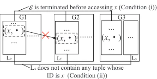
Claim 16. During query processing, given two lists Leand Lt associated with two attributes e and t in different groups, consider a tupleτin list Le. We say that the random access for the tupleτfrom Leto Ltis useless, if there exists a group G (e<G and t<G) such that∀s∈G, either of the two following conditions is satisfied: (i) the list Lsdoes not contain any tupleτ0, s.t.ρ(τ)=ρ(τ0); or (ii) the combinationinvolving s, e and t is terminated.
It is not hard to see Claim 14 and 15 hold. To illustrate Claim 16, let us consider three groupsG1,G2 andG3 in Figure 4, where
G3 contains only two lists. The listLsdoes not contain any tuple
whose ID isx and the combination is terminated. Therefore, according to Claim 16, the random access betweenLeandLtfor
tuple xis unnecessary. This is because no match instances of x
can contribute to the computation of final answers. Note that it is common in real life that some objects are not contained in some list. For example, think of a player who missed some games in the NBA
G1 L ... ... (x,g) ... G2 L ... (x,g) ... G3 L ... H t s
is terminated before accessing x(Condition (i))
L does not contain any tuple whose ID is x (Condition (ii)) ... s (x,g) ... ...
Figure 4: Example to illustrate Claim 16. Assume there are two lists in groupG3. Random access fromLetoLtis useless, since
is terminated andLsdoes not contain any tuple whose ID isx. C1 C2 G1 G2 F1 F2 C1 G1 G2 F1 F2 2 1 1 2 1 1 1 2 2 2 1 2 2 1 2 2 1
(a) initial KMG (b) at depth 2
C1 G1 F1 F2 2 1 1 1 1 (c) at depth 3 (d) at depth 4 1
Figure 5: Example top-k,m graphs (KMG)
pre-season. Furthermore, to maximize the elimination of useless random accesses implied in Claim 16, in our algorithm, we consider theSmall First Access (SFA)heuristic to control the order of random accesses, that is, we first perform random accesses to the lists in groups with less attributes. In this way, the random access across lists in larger groups may be avoided if there is no corresponding tuple in the list of smaller groups. As shown in our experimental results, Claim 16 and the SFA heuristic have significant practical benefits to reduce the number of random accesses.
Summarizing, Claim 14 through 16 imply three levels of gran-ularity to reduce the number of accesses. In particular, Claim 14 eliminates both random accesses and sorted accesses, Claim 15 aims at preventing unnecessary random accesses, while Claim 16 comes in to avoid random accesses for some specific tuples.
In order to exploit the three optimizations in the processing of our algorithm, we carefully design a native data structure namedtop-k,m graph(called KMG hereafter). Figure 5(a) shows an example KMG for the data in Figure 1. Formally, given an instanceΠof the top-k,m
problem, we can construct a node-labeled, weighted graphGdefined as (V,E,W,C), where (1)Vis a set of nodes, eachv∈Vindicating a list inΠ, e.g., in Figure 5, nodeF1refers to the listF1in Figure 1;
(2)E⊆V×Vis a set of edges, in which the existence of edge (v,v0
) means that random accesses betweenvandv0are necessary; (3) for
each edgeeinE,W(e) is a positive integer, which is the weight ofe. The value is the total number of unterminated combinations associated withe; and finally (4)Cdenotes a collection of subsets ofV, each of which indicates a group of lists inΠ, e.g., in Figure 5,
C={{F1,F2},{C1,C2},{G1,G2}}. A path of length|C|inGthat spans
all subsets ofCcorresponds to a combination inΠ.
Based on the above claims, we propose three dynamic operations in KMG: (i) decreasing the weight of edges by 1 if one of combina-tions involving the edge is terminated; (ii) deleting the edge if its weight is 0, which means that random accesses between the two lists are useless (implied by Claim 15); and (iii) removing the node if its degree is 0, which indicates that both sorted and random accesses in this list are useless (implied by Claim 14).
Optimized top-k,m algorithm.
We are now ready to presentthe ULA+algorithm based on KMG, which combines all optimiza-tions implied by Claim 14 to 16. This algorithm is shown as Algo-rithm 2.
Algorithm 2The ULA+algorithm
Input: a top-k,mproblem instance with multiple groups and each groupGhas multiple attributes and each attributenis associated with a listLn.
Output: top-kcombinations of attributes in groups.
(i) Find the seed combinationand prune all useless combina-tions dominated byaccording to the approach in Section 4.4. (ii) Initialize a KMGGfor the remaining combinations. (iii) Do sorted accesses in parallel to lists with nodes inG. (iv) Do random accesses according to the existing edges inG(note
that we need to first access the smaller group based on SFA strategy). In addition, given a tupleτ ∈ Ln,n∈G, if there
is another groupG0such that each node n0in
G0(where∃
edge (n,n0
)∈ G) does not contain the tuple with the same ID ofτ, then we can immediately stop all random accesses forτ (implied by Claim 16).
(v) Computeminandmaxfor each unterminated combination
and determine ifis terminated now by Definition 9 usingmin
andmax. If yes, decrease the weights of all edges involved
inby 1. In addition, remove an edge if its weight is zero and remove a nodev∈ Gif the degree ofvis zero.
(vi) Addto the result setYif it meets the hit-condition. If there are at leastkcombinations which meet the hit-condition, then the algorithm halts. Otherwise, go to step (iii).
(vii) Output the result setYcontaining top-kcombinations.
Example 17. We present an example with the data of Figure 1 to
illustrate ULA+. Consider a top-1,2 query again. Firstly, in step (i), ULA+performs sorted accesses to two rows of all lists, and finds a seed combination, e.g.,F2C1G2, asFmax2C1G2 =40.18<
min F2C1G1=
40.27. Because LC1 LC2, the combination F2C1G2 dominates
F2C2G2. Therefore, bothF2C1G2andF2C2G2can be pruned in step (i).
Then ULA+constructs a KMG (see Figure 5(a)) for non-pruned combinations in step (ii). Note that there is no edge betweenF2and
G2, since bothF2C2G2 andF2C1G2have been pruned. By depth 2,
ULA+computesminandmaxfor each unterminated combination
in step (iii). ThenF1C2G1andF1C2G2meet the drop-condition (e.g.,
max
F1C2G1 =37.6 < min
F2C1G1), and we decrease the weights by 1 for
the corresponding edges, e.g.,w(F1,G1)=1. In addition, nodeC2
should be removed, since all the combinations containingC2are
terminated, (see Figure 5(b)) in step (iv). At depth 3,F1C1G2 is
terminated, sincemax
F1C1G2 =36.48< min
F2C1G1, and we decrease the
weights of (F1,C1), (F1,G2) and (C1,G2) by 1 and remove the node
G2(see Figure 5(c)). Finally, ULA+halts at depth 4 in step (vi) and
F2C1G1is returned as the final result in step (vii). To demonstrate
the superiority of ULA+, we compare the numbers of accessed objects for three algorithms: ETA accesses 54 tuples (at depth 5) and ULA accesses 50 tuples (at depth 4) , while ULA+accesses only 37 tuples (at depth 4) .
4.5
Optimality properties
We next consider the optimality of algorithms. We start by defin-ing the optimality measures, and then analyze the optimality in different cases. Some of the proofs are omitted here due to space limitation; and most proofs are highly non-trivial.
Competing algorithms. LetDbe the class of all databases. We
defineAto be all deterministic correct top-k,malgorithms
running on every databaseD in classD. Following the
access model in [8], an algorithmA ∈Acan use both sorted accesses and random accesses.
Cost metrics. We consider the number of tuples seen by sorted access and random access as the dominant computational
factor. Letcost(A,D) be the nonnegative performance cost measured by running algorithmA over databaseD, which represents the amount of the tuples accessed.
Instance optimality. We use the notions of instance optimality. We say that an algorithmA ∈Aisinstance-optimalif for every
A0∈
Aand everyD∈Dthere exist two constantscandc0
such thatcost(A,D)6c×cost(A0,D
)+c0
.
Following [9], we say that an algorithm makeswild guessesif it does random access to find the score of a tuple with IDxin some list before the algorithm has seenxunder sorted access. For example, in Figure 1, we can see tuples whose IDs areG04 only at depth 3 under sorted and random accesses. But wild guesses can magically find
G04 in the first step and obtain the corresponding scores. In other words, wild guesses can perform random jump on the lists and locate any tuple they want. In practice, we would not normally implement algorithms that make wild guesses. We prove the instance optimality of ULA (and ULA+) algorithm, provided the size of each group is treated as a constant. This assumption is reasonable as it is mainly about assuming that theschemaof the database is fixed.
Theorem 18. LetDbe the class of all databases. LetAbe the class of all algorithms that correctly find top-k,m answers for every database and that do not make wild guesses. If the size of each group is treated as a constant, then ULA and ULA+are instance-optimal overAandD.
Proof. According to the definition of instance optimality, the
main goal of this proof is to show that for everyA ∈Aand every
D∈Dthere exist two constantscandc0
such thatcost(U LA,D)6 c×cost(A,D)+c0
. We obtain the values ofcandc0
as follows. Assume that an optimal algorithmA halts by sorted access at most up to depthd. SinceA needs to access at least one tuple in each list (otherwise we can easily makeA err), the cost ofA is at least (d+Pn
i=1gi−1)Cs, whereCsdenotes the cost of one sorted
access andgiis the number of attributes in the groupGi.
We shall show that ULA halts onDby sorted access at most up to depthd+m. Then the cost of ULA is at most:
Cost6(d+m)(Pn
i=1gi)Cs+(d+m)Pni=1{gi(Pnj=1gj−gi)}Cr =(d+m)(Pn
i=1gi)Cs+(d+m)Pi,j(gigj)Cr
whereCrdenotes the cost of one random access. For simplicity of
presentation, letT =Pn
i=1giandK=Pi,j(gigj). Hence, the cost of
ULA is at most: (d+m)T Cs+(d+m)KCr, which isdT Cs+dKCr
plus an additive constant ofmT Cs+mKCr. So the optimality ratio c= dT Cs+dKCr dCs =T+KCr/Cs. Correspondingly,c 0= mT Cs+mKCr− c(T−1)Cs=(T2+mT−T)Cs+(kT+mK−K)Cr. It is easy to see thatcandc0
are two constants and are independent of the depthd. The following part of the proof aims at showing ULA halts by depthd+m(if the optimal algorithm stops by depthd). LetY
be the output set ofA. There are now two cases, depending on whether or notA has seen the exact top-mmatch instances for each combination when it halts.
Case 1:IfA has seen the exact top-mmatch instances for each combination, then ULA also halts by depthd<d+m, as desired.
Case 2:IfA has not seen the exact top-mmatch instances for each combination, then there are still two subcases depending on whether or not the lower bound of each combination∈Yis larger than the upper bound of the combinations not inYwhenA halts.
Subcase 2.1:For any combination∈Yand combinationξ<Y, min
>ξmax, that is, all the combinations inY meet hit-condition,
and the size ofYisk, so ULA halts by depthd<d+m, as desired.
Subcase 2.2:There exists one combination∈Yand one combi-nationξ<Ysuch thatmin< ξmax. At this point, our ULA algorithm
cannot stop immediately. But sinceA is correct without seeing the remaining tuples after depthd, we shall prove that ULA algorithm accesses at most moremdepths (i.e.,min
>ξmaxat that moment),
otherwise we can easily makeA err.
Given a listLiin a combination, letσi denote the seen minimal
score (under sorted or random accesses) inLiat depthd. Assume
thatA has seenm0
(m0
6 m) match instances for. Letω =
F1(σ1, . . . , σ||) denote the possible minimaltScore. Then we define
anmScoreas follows.
mScore(,m)=F2(tScore(I1), . . . ,tScore(I
m0), ω, . . . , ω | {z } m−m0
)
Assume thatA has seenm00(m006m) match instances forξ. Let
λξ
i denote the unseen possible maximal score (λ
ξ i 6σ(τ)) belowτin listiby depthd+(m−m00 ) ofξ. Letϕ=F1(λ ξ 1, . . . , λ ξ |ξ|) denote the
possible maximaltScore. ThenhScoreis defined as:
hScore(ξ,m)=F2(tScore(Iξ 1), . . . ,tScore(I ξ m00), ϕ, . . . , ϕ | {z } m−m00 )
Let us call a combinationbig if itsmScoreis larger than at least
Ncom−k hScoreof other combinations. We now show that every
memberofYis big. Define a databaseD0
to be just likeD, except object unseen byA. InD0
, assign unseen objectsV1,. . . ,Vmwith
the scoreσi underτin each listLi ∈(∈Y), and assign unseen
objectsU1,. . . ,Umwith the scoreλ
ξ
i underτin a listLj∈ξ(ξ<Y).
ThenA performs exactly the same, and gives the same output and accesses the same objects, for databasesD andD0
. Then by the correctness ofA, it follows that all combinations inYis big.
Therefore by depthd+m, ULA would get at leastmmatch instances, and the lower bound ofis no less thanmS core, and the upper bound ofξis no more thanhS core. SincemS core(,m)> hS core(ξ,m), so by depthd+m,min>ξmax. Therefore, ULA halts
by depthd+m, as desired.
The next theorem shows that the upper bound of the optimality ratio of ULA is tight, provided the aggregation functionsF1andF2
are strictly monotone (the proof is omitted due to space limitation, it can be found in a technical report that cannot be referenced due to the anonymous review).
Theorem 19. Assume thatF1andF2are strictly monotonic
func-tions. Let Crand Csdenote the cost of one random access and one sorted access respectively. There is no deterministic algorithm that is instance-optimal for top-k,m problem, with optimality ratio less than T+KCr/Cs, (which is the exact ratio of ULA), where T =Pn
i=1gi, K =Pi,j(gigj), and gidenotes the number of lists in group Gi.
When we consider the scenarios when an algorithm makeswild guesses, unfortunately, our algorithms are not instance-optimal, but we can show that in this casenoinstance-optimal algorithm exists. Note that this appears a somewhat surprising finding, because the TA algorithm for top-kproblems can guarantee instance optimality even under wild guesses for the data that satisfies the distinct property. In contrast, the ULA algorithm for top-k,mproblem is not instance-optimal even for distinct data. The intuition for this disparity is that top-kproblem needs to return the exactkobjects, forcing all algorithms (including those with wild guesses) to go through the list to verify the results, but an algorithm for top-k,msearch can correctly returnkcombinations without seeing theirmobjects by quickly locating a match instance to instantly boost the lower bound. Theorem 20. LetDbe the class of all databases. LetAbe the class of all algorithms (wild guesses are allowed) that correctly find top-k,m answers for every database. There is no deterministic algorithm that is instance-optimal overAandD.
Finally, we consider the case (not so common in practice) when the number of attributes in each group is treated as a variable. While our algorithm is not instance-optimal in this case, we can show that
noinstance-optimal algorithm exists.
Theorem 21. LetDbe the class of all databases. LetAbe the class of all algorithms that correctly find top-k,m answers for every database. If the number of elements in each group is treated as a variable, there is no deterministic algorithm that is instance-optimal overAandD.
5.
XML KEYWORD REFINEMENT
In this section, we study XML keyword query refinement using the top-k,mframework. We show how to judiciously define the aggregate functions and the join predicates in the top-k,mframework to reflect the semantics of XML keyword search and adapt the aforementioned three algorithms, i.e., ETA, ULA, and ULA+.
5.1
XML keyword refinement
Given a set of keywords and an XML databaseD, we study how
to automatically rewrite the keywords to provide users better and more relevant search results onD, as in real applications users’ input
may not have answers or the answers are not good. In particular, we rewrite the users’ queries by two operations:transformationby rules anddeletion. We assume that there exists a table to contain simple rules in the form ofA→B, whereAandBare two strings. For example, “UC Irvine”→“UCI”, “Database”→“Data base”. These rules can be obtained from existing dictionaries, query log analysis [14], or manual annotation. Given a queryq={q1,. . . ,qn},
we scan all keywords sequentially and perform substring match by rules to generate groups.1For example, assume thatq={UC Irvine,
Database}; then the two groups areG1={UC Irvine, UCI} and
G2={Database,DB}.
We assume that each node in an XML database is assigned with its JDewey identifier [7], which gives the order numbers to nodes at the same level and inherits the label of their ancestors as their prefix. In Figure 2, for example,school(1.2.4) shows that the label of its parent is 1.2 andschoolis the fourth node in level 3 from left to right. One good property of JDewey is that the number is a unique identifier among all nodes in the same tree depth.
In general, to convert the problem of XML keyword refinement to the top-k,mframework, given a keyword queryq={q1,. . . ,qn}, we
first produce a set of groupsG1,. . .,Gtwhere each elementwi j∈Gi
is a keyword associated with an inverted list composed of binary tuplesτ=hρ(τ), σ(τ)i, whereρ(τ) is the JDewey label andσ(τ) is the score of the node (e.g., tf-idf). Then, the XML keyword refinement problem is to return top-kcombinations of keywords that have the best aggregate scores in their top-msearch results.
We now present a widely adopted approach (e.g., [7, 19]) to for-mally definetScoreandcScorein the XML top-k,mproblem. In the XML tree data model, LCA is the lowest common ancestor of multi-ple nodes and SLCA [1] is the root of the subtree containing matches to all keywords without a descendant whose subtree contains all keywords. In particular, given a combinationand tuplesτ1. . . τ||
from different groups, one match instance (i.e., keyword search result) is formed by the SLCA node ˜n=slca(ρ(τ1), . . . , ρ(τ||)). Let xi=σ(τi)×d(li−l˜), wherelidenotes the depth of nodeρ(τi), ˜lis the
depth of ˜n, andd(·) is a decreasing function to leverage the score of SLCA at different levels (e.g.,d(x)=0.9xin our implementation).
We definetScoreto compute the score of one match instanceIas
1In cases where one word (or a set of words) appears in multiple
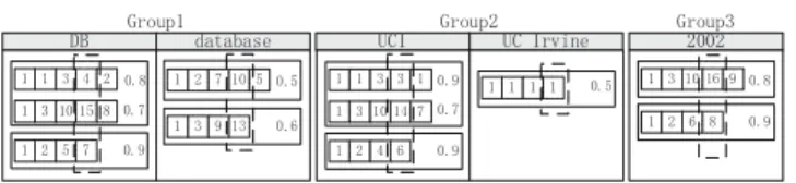
rules, we need to design an algorithm to generate the mapping from words to groups. '% *URXSGDWDEDVH *URXS 8&, 8&,UYLQH *URXS
Figure 6: JDewey labels are clustered by their lengths. The dashed boxes include all data in column 4.
tScore(I)=min(x1, . . . ,x||).Intuitively,tScoreassigns a greater
score to an SLCA subtree with smaller sizes (li −l˜) and higher
weights (σ(τi)).
Given a combinationand an integerm, and thetScores of any
mmatch instancesI1, . . . ,Imon, we define that
cScore(,m)=α|G|−||
×max{tScore(I1)+· · ·+tS core(Im))}
where|G|is the number of groups,||is the number of attributes in the combination, andαis a damping constant (e.g.,α=0.7 in our experiments). The choice of the componentα|G|−||
is to give a penalty fordeletionoperation in keyword refinement in the sense that more deletions (i.e., smaller||) lead to smaller scores.
Compared to the regular top-k,mproblem (in Section 4), XML top-k,mfollows the same framework to return the top-k combina-tions ordered bycScore. But the concrete definitions oftScoreand
cScoreare changed to cater for the tree-specific XML data. There-fore, to address the challenge from SLCA computation, weconvert SLCA subtree computation to ID equi-join in each level. In particu-lar, inspired by [7], we put the nodes into segments by the length of their labels and nodes are ordered by their scores at each level. See Figure 6. For example, in the list of “DB”, data are clustered into two segments by label lengths (i.e., 5 and 4). The dashed boxes show columns corresponding to levels in XML trees, and numbers in one column uniquely identify nodes at that level (this is because of the feature of JDewey labels). In Figure 6, column 4 contains all the 4th JDewey numbers of the nodes. Note that the complete order of one column from different length segments can be reconstructed online, as we can maintain a cursor for each segment and pick one number with the highest score for all the cursors at each iteration. Therefore, to compute SLCA node, in columni, if two numbers have the same valuev, then they share the same prefix path and their LCA subtree is uniquely identified byv. Furthermore, since we access the data in a bottom-up manner in the sense that we first access the column with greater column number, we guarantee that the first seen LCA is the smallest LCA node.
5.2
XML top-k,m algorithms
We now describe how to adapt the previous three top-k,m algo-rithms to work with XML trees. First, the application of ETA on XML (called XETA) is obvious. For each combination of keywords, we compute their exact top-msearch answers and return the top-k
combinations by sorting the finalcScore. Clearly, this approach has to find the top-msearch results forallthe combinations, which is usually prohibitively expensive.
Second, to apply ULA on XML top-k,m, we iteratively access the JDewey numbers by columns in a bottom-up manner, while continuously computing the lower and upper bounds, until all top-k
combinations are found. To compute the upper bound, the tricky issue here is that we access the numbers by columns and do not know the maximal values in other columns. However, this issue can be solved by collecting the scores of top nodes in each col-umn in the preprocessing phase. More precisely, given a term (an attribute)ei and columnl, letylei = max{zl, . . . ,zM}, where Mdenotes the maximal length of nodes in the list ofeiandzj=
sj×d(j−l) (l6j6M), wheresjis the top score of nodes in lengthj
andd(·) has been previously defined. For example, see Figure 6,
y4
DB=max(0.8×0.9
1,0.9×0.90)=0.9, whered(x)=0.9x.
Suppose that we are accessing the JDewey labelτin columnl, and the score of current number (representing an LCA node) can be computed asxl=σ(τ)×d(n−l), wherenis the total number of
components inτ. Given a combination, the threshold valueTl
can be defined as: Tl =min{tle1, . . . ,t l e||} wheretl ei=max{x l ei,y 1 ei, . . . ,y l−1 ei }(16i6||).
For example, in Figure 6, consider a combination “DB”. (Note that a single word can be also considered as a combination due to deletion operation.) Assume that we are accessing the second tuple in column 4, i.e., the current number in list “DB” is 15 and the scorex4 DB =0.7×0.9 (5−4) =0.63, thenT4 =t4DB =max{x 4 DB, y1 DB,y 2 DB,y 3 DB} = max{0.63,0.9 4,0.93,0.92} = 0.81, whereyi DB = max{0.8×0.9(5−i),0.9×0.9(4−i)}.
We present theXULAalgorithm to address top-k,mqueries for XML keyword refinement in Algorithm 3. We iteratively access numbers from different columns in a bottom-up manner.
Algorithm 3The XULA algorithm
Input: an XML top-k,mproblem instance.
Output: top-kcombinations of keywords.
(i) Initialize a variablel=H, the height of XML trees. For each combination, initialize an empty setSto store SLCA nodes and their scores.
(ii) At columnl, sorted access in parallel to each list and do the random accesses to get LCA nodesu. If¬∃p∈S, s.t.uis an ancestor ofp, insertuintoS.
(iii) For each unterminated combination, compute the lower and upper boundsmin andmax (according to the top-mnodes
inS) and check ifis terminated by Definition 9. Prune the combinationby the drop condition (Lemma 7) or confirm to be part of the results by the hit condition (Lemma 8). (iv) LetYbe a set to contain the results. If there arekcombinations
inYor all columns have been accessed, the algorithm halts. OutputY.
(v) If all nodes at columnlhave been accessed,l:=l−1. (vi) Go to step (ii).
Example 22. Given a queryq=hDB,UC Irvine,2002i, we
gen-erate three groupsG1={“DB”,“database”},G2={“UCI”,“UC Irvine”},
andG3 = {“2002”}. See Figure 6. Letd(x)= 0.9xandα =0.7.
Consider a top-1,2 query. In step (i),l=5, depth=1, and there are 17 combinations (not 4, due to the deletion operation) and∀S =∅. In step (ii), the sorted accesses find four (trivial) LCA nodes (single node) (e.g., 1.1.3.4.2 inDB) and add them to the correspondingS. In step (iii), we compute the upper and lower bounds for all 17 combinations. For example,max
DB =0.9α
(3−1)+0.9α(3−1)=0.882,
min DB =0.8α
(3−1)=0.392. Then the conditions in step (iv) and (v) are
not satisfied. Then we are in step (ii) again (l=5, depth=2) and add two new LCA nodes toSDBandSUCIrespectively. In step (iii), at
this moment, five combinations satisfy the drop-condition and are pruned. For example,max
DB,UCIrvine=0.7=2α
(3−2)×min(0.9,0.5),
which is smaller thanmin
DB =0.735=(0.7+0.8)α
(3−1). Thus, the
com-bination “{DB, UC Irvine}” is pruned. Now all nodes in column 5 have been accessed. Subsequently, we access nodes in column 4, 3 and 2. Finally, in column 2, we find the result is the combination “{DB, UCI, 2002}”, which has two SLCA nodes (i.e., 1.3.10 and 1.2) and its lower bound is 0.567+0.729=1.296, which is greater than the upper bounds of all other combinations.
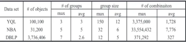
max avg max avg max avg
YQL 100,100 3 3 150 12 3,375,000 1,728
NBA 31,200 5 5 32 6 33,554,432 7,776
DBLP 3,736,406 7 2.6 12 5 371,292 327
# of combinaiton
Data set # of objects # of groups group size
Figure 7: Datasets and their characteristics
Finally, to optimize the XULA algorithm, we can reuse the opti-mizations in ULA+, except Claim 16. This is because XML keyword refinement supports the deletion operation and Claim 16 does not hold when an attribute is allowed to be deleted (recall Figure 4). We have to omit the details of the optimized XULA algorithm (called XULA+) here due to the space limitation, but note that XULA+is implemented and tested in our experiments.
6.
EXPERIMENTAL STUDY
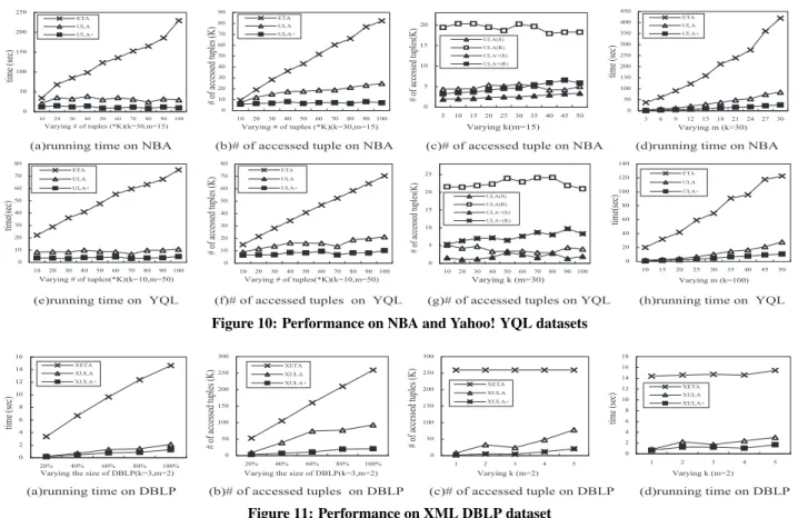
In this section, we report an extensive experimental evaluation of our algorithms, using three real-life datasets. Our experiments were conducted to verify the efficiency and scalability of all three top-k,malgorithms ETA, ULA and ULA+; and their variants for XML keyword query refinement.
Implementation and environment.All the algorithms were imple-mented in Java and the experiments were performed on a dual-core Intel Xeon CPU 2.0GHz running Windows XP operating system with 2GB RAM and a 320GB hard disk.
Datasets. We use three datasets including NBA2, Yahoo! YQL3,
and DBLP to test the efficacy of top-k,malgorithms in the real world. Figure 7 summarizes the characteristics of the three datasets. NBA and Yahoo! YQL datasets were employed to evaluate the
top-k,malgorithms, while DBLP dataset was utilized to test the XML top-k,malgorithms.
NBA dataset.We downloaded the data of 2010–2011 pre-season in NBA for the ”Point Guard”, ”Shooting Guard”, ”Small Forward”, ”Power Forward” and ”Center” positions. The original dataset con-tains thirteen dimensions, such as opponent team, shots, assists and score. We normalized the score of the data into [0,10] by assigning different weights to each dimension. There are five groups, and the average size of each group is about 6.
YQL dataset. We downloaded data about the hotels, restaurants, and entertainments from Yahoo! YQL3. The goal of the top-k,m
queries is to recommend the top-kcombinations of hotels, restau-rants, and entertainments according to users’ feedback. There are three groups, and the average size of each group is around 12.
DBLP dataset. The size of DBLP is about 127M. In order to generate meaningful query candidates, we obtained 724 synonym rules about the abbreviations and full names for computer science conferences and downloaded Babel4data including 9,136 synonym
pairs about computer science abbreviations and acronyms.
Choosing the XML queries. Regarding to the real-world user queries, the most recent 1,000 queries are selected from the query log of a DBLP online demo [3], out of which 219 frequent queries (with an average length of 3.92 keywords) are selected to form a pool of queries that need refinement. Finally, we picked 186 queries that have meaningful refined results to test our algorithms. Here we show 5 sample XML keyword refinement as follows.
Q1:{thomason, huang} is refined by adopting “thomason→thomas”.
Q2:{philipos, data, base} can be refined as {philipos, database}. 2http://www.nba.com/
3http://developer.yahoo.com/yql/console/ 4http://www.wonko.info/ipt/babel.htm