Multi-Issue Negotiation Processes by Evolutionary Simulation
Validation and Social Extensions∗
Enrico Gerding ([email protected]) and David van Bragt ([email protected])
Centre for Mathematics and Computer Science (CWI) P.O. Box 94079, 1090 GB Amsterdam, The Netherlands
Han La Poutr´e ([email protected])
Centre for Mathematics and Computer Science (CWI) P.O. Box 94079, 1090 GB Amsterdam, The Netherlands
School of Technology Management; Eindhoven University of Technology De Lismortel 2, 5600 MB Eindhoven, The Netherlands
May 1, 2002
Abstract. We describe a system for bilateral negotiations in which artificial agents are generated by an evolutionary algorithm (EA). The negotiations are governed by a finite-horizon version of the alternating-offers protocol. Several issues are negoti-ated simultaneously. We first analyse and validate the outcomes of the evolutionary system, using the game-theoretic subgame-perfect equilibrium as a benchmark. We then present two extensions of the negotiation model. In the first extension agents take into account the fairness of the obtained payoff. We find that when the fair-ness norm is consistently applied during the negotiation, agents reach symmetric outcomes which are robust and rather insensitive to the actual fairness settings. In the second extension we model a competitive market situation where agents have multiple bargaining opportunities before reaching the final agreement. Symmetric outcomes are now also obtained, even when the number of bargaining opportunities is small. We furthermore study the influence of search or negotiation costs in this game.
Keywords: multi-issue bargaining, evolutionary algorithms, fairness, multiple bar-gaining opportunities, game theory.
1. Introduction
Automated negotiations have received increasing attention in the last years, especially from the field of electronic trading [4, 14, 15, 17]. In the near future, an increasing use of bargaining agents in electronic market places is expected. Ideally, these agents should not only bargain over the price of a product, but also take into account aspects like the delivery
∗ This paper has been presented at the Workshop onComplex Behavior in
time, quality, payment methods, return policies, or specific product properties. In such multi-issue negotiations, the agents should be able to negotiate outcomes that are mutually beneficial for both parties. The complexity of the bargaining problem increases rapidly, however, if the number of issues becomes larger than one. This explains the need for “intelligent” agents, which should be capable of negotiating successfully over multiple issues at the same time.
In this paper, we consider negotiations that are governed by a finite-stage version of the Rubinstein-St˚ahl multi-round bargaining game with alternating offers [23, 24]. We investigate the computation of strate-gies of the agents by evolutionary algorithms (EAs). EAs are powerful search algorithms (based on Darwin’s evolution theory) which can be used to model social learning in societies of boundedly-rational agents [7, 19]. It is important to note that EAs make no explicit assumptions or use of rationality. Basically, the fitness (i.e., quality) of the individual agents is used to determine whether a strategy will be used in future situations.
A small, but growing, body of literature already exists in this field [15, 17, 25]. These papers demonstrate that, using an EA, artificial agents can learn effective negotiation strategies. In [25], a system-atic comparison between game-theoretic and evolutionary bargaining models is also made, in case negotiations concern a single issue.
The focus of this paper lies on negotiations where multiple issues are involved. We first analyse the results and compare these with game theory. We study both models in which time plays no role and models in which there is a time pressure to reach agreements early (because a risk of breakdown in negotiations exists after each round).
We subsequently present two important extensions of this negotia-tion model. The first extension introduces a fairness norm and is based on the following observation. When no time pressure is present, extreme divisions of the payoff occur in the computational experiments, due to a powerful ‘take-it-or-leave-it’ position for one of the negotiating agents in the last round of the negotiation. Although such extreme outcomes are in agreement with game-theoretic results, they are usually not observed in real-life situations, where social norms such as fairness play an im-portant role [3, 13, 20, 27]. We therefore introduce a fairness norm and incorporate this in the agents’ behaviour. We perform computational experiments with various fairness settings, and show that, depending on the actual settings, “fair” deals indeed evolve.
and is probably a better model of real-life bargaining situations, where often several negotiation partners are available (e.g. within a market place). Because agents now no longer have to accept extreme deals, the situation for agents in a bad bargaining position improves. We perform various experiments with this setup, and we observe efficient and “fair” agreements. We also study the effect of search costs for finding a new negotiation partner.
These evolutionary models are a first attempt to study complex bar-gaining situations which are more likely to occur in practical settings. A rigorous game-theoretic analysis is typically much more involved or may even be intractable under these conditions.
The remainder of this paper is organised as follows. Section 2 gives an outline of the setup of the computer experiments. A comparison of the computational results with game-theoretic results is presented in Section 3. The extensions with fairness and with multiple bargaining opportunities are the topic of Sections 4 and 5 respectively. Section 6 summarises the main results and concludes.
2. Experimental Setup
This section describes the setup of the computational system and ex-periments. The alternating-offers negotiation protocol is described in Section 2.1. Section 2.2 then describes the EA.
2.1. Negotiation Protocol and Agent Model
2.1.1. Negotiation Protocol
During the negotiation process, the agents exchange offers and counter offers in an alternating fashion at discrete time steps (rounds). In the following, the agent starting the negotiations is called “agent 1”, whereas his opponent is called “agent 2”.
Bargaining takes place over missues simultaneously, wheremis the total number of issues. We assume (without loss of generality) that the total bargaining surplus available per issue is equal to unity. We express an offer as a vector~o, where the i-th componentoi specifies the share that agent 1 receives for issue i if the offer is accepted. Agent 2 then receives 1−oi for issue i. The index i ranges from 1 tom. Note that an offer always specifies the share obtained by agent 1.
If negotiations proceed to the next round, agent 2 needs to propose a counter offer, which agent 1 can then either accept or refuse. This pro-cess of alternating bidding continues for a limited number ofnrounds. When this deadline is reached without an agreement, the negotiations end in a disagreement, and both players receive nothing.
2.1.2. Agent Model
The agent model contains the negotiation strategy used by the agent and a utility function to evaluate an opponent’s offer. In a game-theoretic context, a strategy is a plan which specifies an action for each history [2]. In our model, the agent’s strategy specifies the offers ~
oj(r) and thresholds tj(r) for each round r in the negotiation process for agentsj∈ {1,2}. The threshold determines whether an offer of the other party is accepted or rejected: If the value of the offer (see below) falls below the threshold the offer is refused; otherwise an agreement is reached.1 This strategy representation is depicted in Fig. 1. Notice that in each round, the strategy of an agent specifies either an offer or a threshold, depending on whether the agent proposes or receives an offer in that round.
Agent 1 ~o1(1) t1(2) ~o1(3) t1(4) . . .
Agent 2 t2(1) ~o2(2) t2(3) ~o2(4) . . .
Figure 1. The strategies for agentj ∈ {1,2}specify a sequence of offers~oj(r)
and thresholdstj(r) for roundsr∈ {1,2, . . . , n}of the negotiation.
The agents evaluate the offers of their opponents using an additive multi-attribute utility function [15, 17]. Agent 1’s utility function is
~
w1 ·~oj(r) = Pmi=1wi1·oij(r), where j = 1 if the offer is proposed by agent 1 andj= 2 otherwise. Agent 2’s utility function isw~2·[~1−~oj(r)]. Here, w~j is a vector containing agent j’s weights wij for each issue i. The weights are normalised and larger than zero, i.e.,Pm
i=1wij = 1 and wji ≥ 0. Because we assume that 0 ≤ oij(r) ≤ 1 for all i, the utilities are real numbers in [0,1].
2.2. The Evolutionary System
We use an EA to evolve the negotiation strategies of the agents. The implementation is based on “evolution strategies”(ES), using a
real-1
encoding of the offers and thresholds [1].2 A technical description of our implementation is given in Appendix A. An outline of the EA is given in Fig. 2.
Offspring
Population 2 Population 1
Population 2
Offspring
negotiate
reproduce reproduce
Population 1
Population 2 replace
negotiate
Population 1 Parental
Parental
New parental
New parental
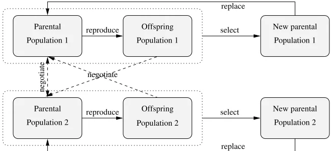
[image:5.595.136.462.146.295.2]replace select select
Figure 2. Iteration loop of the evolutionary algorithm.
The system initially starts with two separate (and randomly ini-tialised) “parental” populations of bargaining agents. Each agent within a population contains a bargaining strategy, which is encoded on his “chromosome” as a set of real values. These values specify the offers for each round and for each issue separately, and also the thresholds for each round (see Appendix A.1).
Agents in population 1 start the bargaining process (i.e., they are of the “agent 1” type). The fitness of the parental agents is determined by negotiation between the agents in the two parental populations. Each agent negotiates with all agents in the other population. The utility functions are the same for agents within the same population (i.e., the weight settings are equal). The average utility obtained in all negotiations is an agent’s fitness value.
Subsequently, “offspring” agents are created (see Fig. 2). An off-spring agent is generated by first (randomly, with replacement) se-lecting an agent in the parental population, and then mutating his chromosome to create a new offspring (see Appendix A.2). The fitness of the new offspring is evaluated by negotiation with the parental agents.3 A social or economic interpretation of this parent-offspring interaction is that new agents can only be evaluated by competing against existing or “proven” strategies.
2
The widely-used genetic algorithms (GAs) are more tailored toward binary-coded search spaces [11, 16, 9].
3
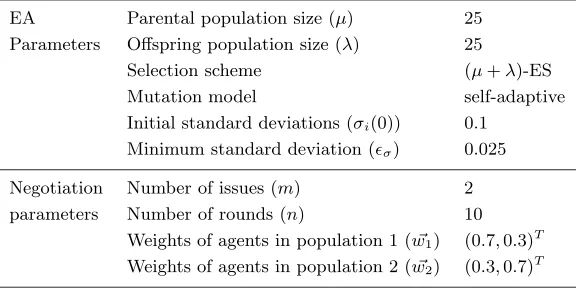
In the final stage (see Fig. 2), the fittest agents from the parental and offspring populations are selected as the new “parents” for the next iteration (see Appendix A.3). This final step completes one iteration (or “generation”) of the EA. All relevant settings of the evolution-ary system are listed in Table I (further explanation is provided in Appendix A).
Table I. Default settings of the evolutionary system.
EA Parental population size (µ) 25 Parameters Offspring population size (λ) 25
Selection scheme (µ+λ)-ES Mutation model self-adaptive Initial standard deviations (σi(0)) 0.1
Minimum standard deviation (σ) 0.025
Negotiation Number of issues (m) 2 parameters Number of rounds (n) 10
Weights of agents in population 1 (w~1) (0.7,0.3) T
Weights of agents in population 2 (w~2) (0.3,0.7) T
3. Validation and Interpretation of the Evolutionary Experiments
Experimental results obtained with the evolutionary system are pre-sented in this section. A comparison with game-theoretic results is made to validate the evolutionary approach. Section 3.1 addresses the evolution of efficient negotiation results. Section 3.2 further analyses the results and compares the experimental results with predictions from game theory. In the following, we refer to the agents in the evolutionary system as “evolutionary agents”.
3.1. Efficiency
agents avoid disagreements by reaching agreements early: after 1000 generations, approximately 75% is reached in the first round.
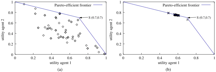
Next, we study the efficiency of the agreements reached in the ex-periments. The agreements are depicted in Fig. 3. This figure shows the utilities for both agents of the deals reached. Also depicted in Fig. 3 is the so-called “Pareto-efficient frontier”. An agreement is located on the Pareto-efficient frontier when an increase of utility for one agent nec-essarily results in a decrease of utility for the other agent. Agreements can therefore never be located above the Pareto-efficient frontier. A special point is the symmetric pointS [at (0.7,0.7)], where both agents obtain the maximum share of the issue they value the most, and receive nothing of the less important issue.
0 0.2 0.4 0.6 0.8 1
0 0.2 0.4 0.6 0.8 1
utility agent 2
utility agent 1
Pareto-efficient frontier
S (0.7,0.7)
(a)
0 0.2 0.4 0.6 0.8 1
0 0.2 0.4 0.6 0.8 1
utility agent 2
utility agent 1
Pareto-efficient frontier
S (0.7,0.7)
[image:7.595.69.529.261.416.2](b) Figure 3. Agreements reached by the evolutionary agents at (a) the start of a typical EA run and (b) after 100 generations. The negotiation settings are
p= 0.7 andn= 10.
Figure 3 shows that initially, many agreements are located far from the Pareto-efficient frontier. After 100 generations, however, the agree-ments are chiefly Pareto-efficient. We note that, even in the long run, the agents keep exploring the search space, resulting in a continuing moving “cloud” of agreements along the frontier.
Conclusion. Results in this section thus show that the evolutionary agents reach efficient agreements, viz. on the Pareto-efficient frontier, and that disagreements are avoided. The next section studies the actual outcomes more closely, using results from game theory as a benchmark.
3.2. Further Analysis
if they constitute a Nash equilibrium in any subgame that remains after an arbitrary sequence of offers and replies. Rubinstein and (much earlier) St˚ahl applied this notion to the alternating-offers bargaining game [23, 24]. Our experimental setup differs in two respects from their model, however. First, the agents bargain over multiple issues instead of a single issue. Second, the evolutionary agents are “myopic”: they do not apply any explicit rationality principles in the negotiation process, nor do they maintain any history. Actually, they only experience the profit of their interactions with other agents. The SPE behaviour of rational agents with complete information will nevertheless serve as a useful theoretical benchmark.
We distinguish between three classes of experiments w.r.t. the break-down probability: (1) no risk of breakbreak-down (p= 1), (2) a low breakdown probability (0.8 ≤ p < 1.0) and (3) a high breakdown probability (p < 0.8). For each of these classes we consider the role of n on the outcomes.
We found that in our experiments, when p = 1, in the long run almost all agreements are delayed until the last round (about 80% after 1000 generations). Furthermore, the last offering agent makes a take-it-or-leave-it deal and demands almost the entire surplus (on each issue), which is accepted by the opponent. This extreme division of the surplus agrees with game-theory [8]; it is rational for the responder to accept any positive amount in the last round. Note, however, that rational agents are indifferent about the actual round in which the agreement is reached. The deadline-approaching behaviour in our experiments corresponds better to “real-world” behaviour [21], however.
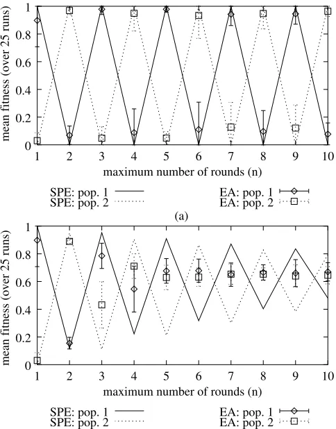
The EA results and SPE outcomes for different values of n (game length) are compared in Fig 4a. To guide the eye, the SPE outcomes for successive values ofnare connected. Notice that fitness of agents in population 1 converges to unity if nis odd, and to to zero ifn is even (the opposite holds for the agents in population 2).
0 0.2 0.4 0.6 0.8 1
1 2 3 4 5 6 7 8 9 10
maximum number of rounds (n) SPE: pop. 1
SPE: pop. 2 EA: pop. 1EA: pop. 2
mean fitness (over 25 runs)
(a)
0 0.2 0.4 0.6 0.8 1
1 2 3 4 5 6 7 8 9 10
maximum number of rounds (n) SPE: pop. 1
SPE: pop. 2 EA: pop. 1EA: pop. 2 (b)
[image:9.595.179.421.95.404.2]mean fitness (over 25 runs)
Figure 4. Comparison of the long-term evolutionary results with SPE results
for (a)p= 1 (time indifference) and (b)p= 0.95. The error bars indicate the
standard deviations across 25 runs.
continues to explore other strategies, which results in a remaining small number of disagreements (see Section 3.1).
Asp becomes smaller, the influence of the game length on the SPE outcome also decreases (see [25]). Therefore, if p becomes sufficiently small (e.g., p < 0.8), the computational results automatically show a much better match with SPE outcomes than if pis large: the match is almost perfect, although a small number of disagreements occur due to a continuing exploration of new strategies.
finite-horizon model forn≥5 (see Fig. 4b). The same behaviour was observed for other EA settings (e.g., larger population size) and other negotiation situations (e.g., other weight settings).
We also studied the performance of the EA in case the number of issues m is increased to 8.4 We observe that, for p= 1, the long-term outcomes of the EA are unstable and do not converge to the extreme partitioning. When we increase the population size for the EA from 25 to 100 agents,5 the extreme partitioning reappears. Thus, for more complicated bargaining problems, the EA parameters must be adjusted. For m = 8 and p < 1, similar observations are found as reported in Section 3.2 (like Fig. 4) when using the adjusted population size.
Conclusion.Game-theoretic (SPE) results appear to be a very useful benchmark to investigate the results of the evolutionary simulations. In computational simulations without a risk of breakdown (case 1), agreements are predominantly reached in the final round. This deadline effect is consistent with human behaviour [21]. Furthermore, the last agent in turn successfully exploits his advantage and claims a take-it-or-leave-it deal (as in SPE). In case of a small risk of breakdown (case 2), the deadline is not accurately perceived by the evolving agents, and the last-mover advantage is smaller than predicted by game theory. In fact, if the finite game becomes long enough, results match the SPE outcomes for the infinite-horizon game. With a high risk of breakdown (case 3), however, this deviation from SPE becomes negligible. Finally, it appears to be important to adjust the EA parameter settings (e.g., by increasing population sizes) for more complex bargaining problems.
4. Social Extensions: Fairness
We extend the agent model within our evolutionary system in this section to study the influence of “fairness”, an important aspect of real-life bargaining situations. The motivation and description of this fairness model is given in Section 4.1. In the fairness model studied in Section 4.2 the evolving agents only take the fairness of a proposed deal into account when the deadline is reached. Section 4.3 presents results obtained when agents perform a “fairness check” in each round. Section 4.4 further analyses the model in Section 4.3 for a simple case.
4
The 8-dimensional weight vector for agents in popula-tion 1 is set to 1
3.9(0.7,0.3,0.5,0.2,0.3,0.4,0.5,1.0) T
and equal to
1
3.9(0.3,0.7,0.5,1.0,0.5,0.5,0.2,0.2) T
for agents in population 2. These settings are such that they contain both “competitive” issues (e.g., issue 3) and issues where compromises can be made (e.g., issue 8).
5
4.1. Motivation and Description: the Fairness Model
Game-theoretic models for rational agents often predict the occurrence of very asymmetric outcomes for the two parties. We showed in Sec-tion 3.2 (see Fig. 4a) that such “unfair” behaviour can also emerge in a system of evolving agents, in particular when p = 1 or n is small (see Fig. 4). Large discrepancies between human behaviour in labo-ratory experiments and game-theoretic outcomes are found, however, both for ultimatum (1 round) and multi-stage (several rounds) games [3, 6, 13, 20, 22, 27]. A possible explanation for the occurrence of these discrepancies between theory and practice is the strong influence of so-cial or cultural norms on the individual decision-making process. In [20, p. 264] and [10], for example, it is argued that responders tend to reject unfair or “insultingly low” proposals. Therefore, an anticipating agent should lower his demand in order to avoid a disagreement, this way taking into account the expectations about his opponent’s behaviour.
In [13] a model is proposed in line with this hypothesis. In their model, the probability of acceptance of an offer increases with the amount offered to the responder. Such a model, making more realistic assumptions about the agents’ behaviour, appears to organise the data from experiments with humans better than the SPE model [13].
Following [13], we introduce a fairness model in our evolutionary system. The agent model (see Section 2.1.2) is extended as follows. If the value of an offer exceeds the responder’s threshold, the agent has the opportunity to re-evaluate his decision. The probability that he finally accepts the agreement is then a function of the acquired utility. This so-called “fairness function” is assumed to be piece-wise linear (with up to three segments).6 The instances that we use are shown in Fig. 5.7 We now further distinguish between two different extended agent models. In the first model, the fairness function is used at the deadline only. This situation is studied in Section 4.2. In the second model, the fairness function is effective at any moment. This case is studied in Section 4.3. The first case is motivated by the deadline-effect observed in the experiments without a risk of breakdown (see Section 3.2), where most agreements are reached in the last round. The second case, however, is more likely to be an appropriate model of human behaviour.
6
Piece-wise linear functions nicely fit the experimental data reported in [13, 22].
7
0 1
4 3 1
2 3
4
5
utility responder0.5 1 0.5
probability of acceptance
1
0
0 (no fairness check)
2 (average fairness)
[image:12.595.143.453.86.211.2]5 (greedy behaviour)
Figure 5. Fairness functions used by the agents in the EA.
4.2. Fairness Check at the Deadline
In this section, fairness is applied in the last round. We study the case in which p = 1 and n= 3. Figure 6 shows that if the evolving agents in population 2 use fairness function 1 (i.e., a “weak” fairness model), the partitioning is much less extreme than in case of no fairness check (function 0). However, the agents in population 1 still reach a relatively high fitness (utility) level. Fair agreements evolve, on the other hand, when the agents in population 2 use function 2 (a case with average fairness). In this case the mean long-term fitness is approximately equal to 0.7 for all agents (most agreements are thus located close to the symmetric point S in Fig. 3).
0 0.2 0.4 0.6 0.8 1
0 50 100 150 200 250 300
generation
mean fitness (over 25 runs)
0 (pop. 1)
5 (pop. 2)
4 (pop. 2) 1 (pop. 1) 3 (pop. 2)
2 (pop. 1) 2 (pop. 2)
3 (pop. 1)
4 (pop. 1)
1 (pop. 2)
5 (pop. 1)
0 (pop. 2)
Figure 6. Mean fitness when fairness functions 0-5 are applied at the deadline.
[image:12.595.169.422.413.563.2]demand a larger share of the surplus in the round before last. As a result, the deadline is effectively reached one round earlier. This effect indeed occurs in our experiments.
Conclusion. Our results show that fair outcomes can evolve in an evolutionary system with a fairness model in the last round. However, there is a rather large sensitivity to the actual fairness function that is used by the evolved agents; an “average” fairness function yields symmetric results, whereas more extreme fairness functions yield more asymmetric outcomes.
4.3. Fairness Check in Each Round
This section studies the second fairness model, in which the responding agent re-evaluates all potential agreements. The EA settings are the same as in the previous section.
The results in Fig. 7 for fairness functions 1 are similar to the pre-vious case (see Fig. 6). However, when fairness functions 2 through 5 are used, the agents in both populations reach almost identical fitness levels. Most agreements now occur in the vicinity of point S in Fig. 3. Note that the agents have no explicit knowledge about the location of this point, and that this knowledge is also not incorporated within the fairness functions. We also observe that agreements are now reached in different rounds, whereas in earlier experiments without fairness most agreements occur at the very end of the game.
Fig. 7 thus shows that the agents’ long-term behaviour is much less sensitive to the shape of the fairness function: the various “stronger” fairness functions all yield similar results. Figure 7 however indicates that when the agents use fairness function 5, the mean fitness of both agents decreases. This is due to the increasing number of disagreements which are a result of the strong fairness check.
We furthermore studied a 2-issue negotiation problem with an asym-metric Pareto-efficient frontier, as shown in Fig. 8. In this case, agent 1 values both issues equally important, whereas agent 2 has different valuations for each issue (his weights are 0.2 and 0.8 for issues 1 and 2 respectively). If each agent obtains the whole surplus on his most important issue, agent 1 obtains 0.5, whereas agent 2 gets 0.8. This outcome corresponds to the Nash bargaining solution (NBS) [2, Ch. 5]. The symmetric point (S), on the other hand, is located at (138,138).8
Both solutions can be considered to be fair outcomes in different ways: the first solution maximises the product of the agents’ utili-ties and also splits the surplus equally, whereas in the second case equal utility levels are obtained for both agents (see [18, Ch. 16] for
8
0 0.2 0.4 0.6 0.8 1
0 50 100 150 200 250 300
2 3 4 0 (pop. 1)
1 (pop. 1)
5 (pop. 2) 5 (pop. 1) 1 (pop. 2)
0 (pop. 2)
generation
[image:14.595.170.426.91.248.2]mean fitness (over 25 runs)
Figure 7. Mean fitness when fairness functions 0-5 are applied each round.
0 0.2 0.4 0.6 0.8 1
0 0.2 0.4 0.6 0.8 1
utility agent 2
utility agent 1
Pareto-efficient frontier
S(8/13,8/13) NBS(0.5,0.8)
Figure 8. Resulting agreements in a single generation when the Pareto-efficient frontier is asymmetric and fairness function 4 is used.
a related discussion). In the computational results, we observe that, when fairness functions 2-5 are applied, the agreements are divided and are usually concentrated in two separate clusters (“clouds”), see Fig. 8. The issue of the choice of and distribution over multiple “fair” agreement points seems an important issue for further research, both in a computational setting as well as in experimental economics.
We also experimented with different weight vectors and with m > 2. A general finding is that extreme outcomes do not occur in the evolutionary process if the agents apply a fairness check.
[image:14.595.187.415.280.441.2]Table II. Comparison of the agents’ payoffs in the EA with SPE results.
Payoff agent 1 Payoff agent 2
SPE 0.419 0.391
EA 0.391 (±0.022) 0.412 (±0.014)
if a very strong fairness function is used, resulting in a lower fitness for both parties. In case of two-issue negotiations with a symmetric Pareto-efficient frontier, most agreements are reached in the vicinity of the symmetric point. In the asymmetric case, fair solutions can also be obtained. The solutions are then distributed over various possible outcomes, which can all be considered fair in different ways.
In the next section, we investigate the evolving strategies of the agents in more detail, but for single-issue negotiations.
4.4. Validation and Strategy Analysis for a Simple Case
Although our incorporation of fairness aspects makes a game-theoretic analysis much more complicated, SPE strategies can again be derived for a very simple version: the game with only a single issue (m= 1) and fairness function 4. These settings were chosen because of mathematical feasibility. The general equations are presented in Appendix B.
Table II shows both the SPE results and the payoffs obtained by the evolving agents (in the long run) in the a with m = 1, n = 3, p= 1, and with the (rather strong) fairness function 4. Note that since m= 1, an agent’s payoff equals the share obtained for issue 1. Results for the EA are obtained after 300 generations (averaged over 25 runs). Notice that the SPE payoffs are in good agreement with the outcome of the evolutionary experiments. However, in SPE agent 1’s payoff is slightly larger than agent 2’s payoff. In the EA this is reversed, although Table II shows that differences between theory and experiment are very small. We will further analyse the evolving strategies below.
Table III compares the offers of the evolving agents (for each round) with SPE results, showing a good match. From Table III, it can be derived that agreements are reached inall rounds, with some emphasis on the first round.9
Table III also shows the acceptance thresholds (the thresholds are calculated based on the payoff which an agent expects to receive if he
9
Table III. Comparison of the evolved strategies with game-theoretic (SPE) results for each round.
Round Offer Offer Threshold Threshold (SPE) (EA) (SPE) (EA)
1 0.609 0.58±0.06 0.391 0.23±0.21 2 0.375 0.39±0.07 0.250 0.14±0.13 3 0.500 0.48±0.09 0.000 0.13±0.13
rejects the current offer, see Appendix B). Because the thresholds in rounds 2 and 3 are much lower than the obtained utility, the thresholds in these rounds are not really relevant in SPE. This explains the large variance of the thresholds in the EA and why these thresholds can de-viate from SPE predictions in these rounds. In round 1, the threshold is important in SPE and influences the offer made. The experiments show a much lower average threshold value than the SPE (see Table III). Nevertheless, the thresholds influences the offers made in the EA due to a high variance of the threshold values. We analyse this more closely.
0 0.2 0.4 0.6 0.8 1
0 200 400 600 800 1000
mean threshold population 2 (round no. 1)
[image:16.595.177.418.379.550.2]generation
Figure 9. Average threshold values of the agent strategies in the EA in the first round.
In order to obtain an even better match with SPE results, we re-duced the occurrence of frequent peaks by using a decreasing mutation step-size in the EA (instead of self-adaptive mutation step-sizes, see Appendix A.2). At the beginning of each EA run, σi is set to 0.1 for all i (as before, see Table I) and then exponentially decrease until σi = 0.01 after 1000 generations. This procedure indeed reduces the fluctuations in the threshold values and the offers in the long run. Results for experiments with this EA setting appear to be in excellent agreement with SPE results, see Table IV. We found no significant effect of the new mutation scheme on the evolutionary outcomes for m = 2, however. We suspect that this is due to the integrative nature of the negotiation problem, where the results obtained are already beneficial for both parties.
Table IV. Comparison of the evolutionary agents’ payoffs after 1000 generations (using exponentially decreasing mu-tation step-sizes) with SPE results
Payoff agent 1 Payoff agent 2
SPE 0.419 0.391
EA with decreasingσi 0.416±0.012 0.395±0.009
Conclusion.This relatively simple bargaining situation shows a good match between theoretical (SPE) and experimental results. Further-more, when fairness norms are applied, the outcome of the negotiation process comes to depend on the actual round in which an agreement is finally reached, while thresholds play an important role in some of the rounds. We also showed that EA parameters can be fine-tuned for a more stable situation if needed. This rendered an excellent match with the SPE form= 1.
5. Social Extensions: Multiple Bargaining Opportunities
from the bargaining behaviour of all competitors. This makes an an-alytical treatment extremely difficult compared to the easier case of one-on-one negotiations. Below, we describe the game in more detail and discuss the results of the simulations.
5.1. Description of the Game
As before, we model a society with two groups of agents (e.g. buyers and sellers), which correspond to the two populations in our EA. In the extended game, every agent within either population can subsequently bargain with up to k opponents to reach a deal. A simple bargaining game is denoted as an “encounter” in the following and we use “m-game” to denote a game with multiple bargaining opportunities. If an encounter does not result in an agreement, an agent is again matched with a randomly selected opponent for his next encounter (provided that the agent still has another bargaining opportunity). Thus, an agent can now refuse offers which are unsatisfactory and wait for a better deal in another encounter, which is usually played against a different opponent.
We also introduce search costs in our model. The search costs rep-resent the amount of money, time, or effort that an agent may incur in finding another negotiation partner [5, Ch.7]. These costs, however, can also represent the costs involved in the negotiation process itself. Search costs are fixed and associated with each new encounter (only the first encounter is “free”).
5.2. Implementation
The m-game is implemented as follows. First, a pair of agents is ran-domly selected from the populations and negotiate using the alternating-offers protocol as before, where agent 1 makes the first offer and agent 2 either rejects or accepts. We taken= 1, i.e., just one round of bargain-ing. This is justified based on the results in Section 3.2, where it was observed that each agreement was completely determined by the last round only. If agent 2 refuses the deal, the bargaining ends, and the agents can participate in another encounter, provided that they have not exceeded their maximum number of bargaining opportunities. An agent incurs some fixed costs (which could be zero) for locating another negotiation partner. If an agent has no more bargaining opportunities or if an agreement is reached, this concludes an agent’s m-game and he is disactivated.
agents are randomly matched, two encountering agents may differ in their remaining number of bargaining opportunities. Therefore, the bargaining position of the opponent is not known.
To reduce stochastic effects and to remove initiatory and end effects (explained below), each agent actually plays a number of consecutive m-games in the simulation: If an m-game is concluded, the agent starts with a new m-game. A distinct payoff results from each m-game. The maximum number of m-games that an agent can play is fixed to 10.
The fitness of an agent is the average payoff obtained in his m-games. However, since initially all agents of both populations start with their first encounters, in the first rounds of the encounters the opponent’s bargaining position is not completely random (i.e., there is an initiatory effect). Furthermore, we note that when one of the populations has no more active agents, the other population may still be active (i.e., there is also an end effect). To suppress these undesired effects, we do not include an agent’s payoff received in the first m-game and the last four m-games when calculating his fitness value. This way, we model an ongoing bargaining society.
5.3. Agent Model
[image:19.595.181.415.510.552.2]The strategy representation and the utility function of Section 2.1.2 are somewhat altered in the m-game. Agent 1’s negotiation strategy now consists ofkoffers, one for each encounter, and agent 2 haskthresholds (wherekis the maximum number of encounters). The utility functions are changed tow~1·~oj(e)−σ1·(e−1) andw~2·[~1−~oj(r)]−σ1·(e−1) for agent 1 and 2 respectively, where σj is agent j’s search cost and e ∈ {1,2, . . . , k} counts the opponents. Notice that an agent’s payoff can also become negative.
Table V. Settings for the experiments with multiple bargaining opportunities.
Maximum number of encounters per m-game (k) 1-20 Maximum number of m-games 10 M-games used for fitness evaluation 2-6
5.4. Results without Search Costs
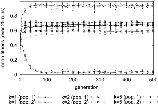
in Fig. 10. The agents reach agreements near the symmetric point (see Fig. 3) whenk= 5, in contrast to the take-it-or-leave-it deals observed when k= 1. The last-mover advantage appears to diminish rapidly if agents are allowed additional bargaining opportunities, even for k= 2 (see Fig. 10). In fact, three encounters are already sufficient to obtain almost symmetric fitness values. Furthermore, this symmetry remains for larger values of k (experiments have been performed with k up to 20). These outcomes are also robust for various other EA settings.
0 0.2 0.4 0.6 0.8 1
0 100 200 300 400 500
mean fitness (over 25 runs)
generation
k=1 (pop. 1)
k=1 (pop. 2) k=2 (pop. 1)k=2 (pop. 2)
[image:20.595.171.428.214.384.2]k=5 (pop. 1) k=5 (pop. 2)
Figure 10. Evolving fitness value fork= 1,k= 2 andk= 5.
We also performed experiments using the asymmetric Pareto-efficient frontier shown in Fig. 8. Results in generation 500 of a typical run are shown in Fig. 11. Recall from Section 4.3 that the bargaining game has two fitness outcomes which are specific candidates for a “fair” outcome: the symmetric point and the Nash bargaining solution. Figure 11 shows that most agreements in the simulation with multiple bargaining op-portunities are located in between both bargaining solutions, and that thus fair deals emerge.
Conclusion. We show that competition among agents induced by multiple bargaining opportunities results in “fair” agreements. These results are obtained without any additional constraints on the agent model.
5.5. Influence of Search Costs
0 0.2 0.4 0.6 0.8 1
0 0.2 0.4 0.6 0.8 1
utility agent 2
utility agent 1
Pareto-efficient frontier
S(8/13,8/13) NBS(0.5,0.8)
Figure 11. Resulting agreements (after 500 generations) when the Pareto-efficient frontier is asymmetric and the agents have 5 bargaining opportunities.
proposing agent to be able to make an extreme take-it-or-leave-it deal as before. These results are indeed found in the simulation: if the search costs are greater than unity, agent 1 will receive almost the whole surplus.
Similar results, however, are also obtained for much smaller search costs, see Fig. 12. This figure shows the fitnesses after 1000 generations of both agent populations for experiments with k = 2,5 and different (but symmetric) search costs. Even when search costs are relatively small, the agents are stimulated to reach agreements early. Notice that, even if search costs are as low as 0.05, the utility of agent 2 decreases from≈0.68 (without search costs) to≈0.15 whenk= 5. This decrease in fitness of ≈0.53 is much larger than the possible total search costs (0.2 in case of 5 encounters). Thus, the search costs have a “leverage” effect on the outcome of the bargaining process.
Conclusion. Without search costs or with very small search costs, fair deals occur. If agents incur more substantial search costs, however, a leverage effect may result in extreme deals as before.
0 0.2 0.4 0.6 0.8 1
0 0.05 0.1 0.15 0.2
mean fitness (over 25 runs)
search costs
k=2 (pop. 1)
[image:22.595.174.418.152.323.2]k=2 (pop. 2) k=5 (pop. 1)k=5 (pop. 2)
Figure 12. Long-term EA results for varying (symmetric) search costs fork= 2 and k= 5.
6. Conclusions
We have investigated a system for negotiations, in which agents learn effective negotiation strategies using evolutionary algorithms (EAs). Negotiations are governed by a finite-horizon version of the alternating-offers game. Several issues are negotiated simultaneously. Both negotia-tions with and without a risk of breakdown have been studied. Our ap-proach facilitates the study of cases for which a rigorous mathematical approach is unwieldy or even intractable. We presented computational results for several difficult bargaining problems in this paper.
We first validated the long-term evolutionary behaviour using the game-theoretic concept of subgame-perfect equilibrium (SPE). When no risk of breakdown exists, the last agent in turn proposes a take-it-or-leave-it deal in the last round and demands most of the surplus for each issue. This extreme division is consistent with SPE predictions. When a risk of breakdown exists, most agreements in the EA are reached in the first round. If the finite game becomes long enough, the deadline is therefore no longer perceived by the evolutionary agents and results actually match SPE predictions for the infinite-horizon game.
al-lowing for multiple bargaining opportunities. In the first extension, a responding agent carries out a fairness check before an agreement is definitely accepted. This fairness check was modelled in two ways: a responding agent considers fairness only at the deadline or all the time, for any potential agreement. In both cases, fair outcomes can be obtained but the outcomes in the second case are much less sensitive to the actual choice of the fairness function. In case of an asymmetric bargaining situation (where the players have asymmetric preferences), multiple outcomes then exist which can be considered “fair” in different ways. We also found a good match between the EA results and game-theoretic SPE predictions for a simple bargaining game (concerning a single issue).
In the second extension, each agent is allowed to subsequently ne-gotiation with a number of opponents and therefore has several oppor-tunities to reach an agreement. It appears that agents now no longer propose a take-it-or-leave-it deal and fair agreements spontaneously emerge in the evolutionary system. This effect is reduced when agents incur some more substantial search costs, and results then again show an unequal partitioning of the bargaining surplus.
Appendix APPENDIX
A. Technical Description of the Evolutionary Algorithm
A.1. Genetic Representation of the Strategies
The chromosome specifies the strategy which an agent uses in the bargaining game. A chromosome consists of a sequence of real values in the unit interval for the offers and thresholds (one offer or threshold for each negotiation round). We use xi to denote the (real) value at location i of the chromosome. The agents’ strategies are initialised at the beginning of each EA run by drawing random numbers in the unit interval (from a flat distribution).
A.2. Mutation and Recombination
Mutation and recombination are the most commonly used EA opera-tors for reproduction. Recombination exchanges parts of the parental chromosomes, whereas mutation produces random changes in a chro-mosome. Earlier experiments [25] showed little effect on the results when a recombination operator was applied. We therefore focus on mutation-based models.
The mutation operator changes the chromosome of an agent as fol-lows. Each real value xi is mutated by adding a zero-mean Gaussian variable with a standard deviation σi [1, 25]:
x0i :=xi+σ0iNi(0,1). (1)
All resulting values larger than unity (or smaller than zero) are set to unity (respectively zero). In our simulations, we use an elegant mutation model with self-adaptive control of the standard deviations σi [1, pp. 71-73][25]. This model allows the evolution of both the strategy and the corresponding standard deviations at the same time. More formally, an agent consists of strategy variables [x0, ..., xl−1] and ES-parameters [σ0, ..., σl−1] in our model, wherel is the length of the chromosome.
The mutation operator first updates an agent’s ES-parametersσi in the following way:
σi:=σiexp[τ0N(0,1) +τ Ni(0,1)], (2)
zero and standard deviation one. The index iinNi indicates that the variable is sampled anew for each value ofi. We use commonly recom-mended settings for these parameters.10 After the strategy parameters have been modified, the strategy variables are mutated as indicated in Eq. 1. The initial standard deviations σi in the EA are set to a value of 0.1. The particular initial value chosen forσi is typically not crucial, because the self-adaptation process rapidly scales σi into the proper range. To prevent complete convergence of the population, we force all standard deviations to remain larger than a small value εσ = 0.025 [1, pp. 72–73].
A.3. Selection Model
Selection is performed using the (µ+λ)-ES selection scheme [1], where µ is the number of parents andλis the number of generated offspring (µ=λ=25, see Table I). The µ survivors with the highest fitness are selected (deterministically) from the union of parental and offspring agents.
B. Game-Theoretic Analysis of Multi-Issue Negotiations
Subgame perfect equilibrium (SPE) strategies for multiple-stage games with complete information can be derived using a backward induction approach. The fairness models evaluated in Section 4.2 (i.e., with a fairness check at the deadline only) and in Section 4.3 (i.e., with a fairness check in each round) are analysed in this appendix. As in [8, 25], we apply backward induction to deduce the SPE partitioning. The fairness function is now formally denoted as gr(u). This (real-valued) function returns the probability of acceptance of a proposal in roundr in case the responding agent’s utility is equal to u. If a fairness check is performed only in the last round,gr(u) = 1 for allr < n(wherenis the number of rounds). In case the same fairness check is performed each round, gr(u) is independent of r. We assume that the fairness function is a monotonic non-decreasing function of u and that gr(u = 1) = 1. Let agent j be the agent proposing a deal at round r and agent −j the responder. We then abbreviate gr[u−j(~oj(r))] (the probability of acceptance of agent j’s offer~oin roundr) as paccr (~o).
Ifnis even, agent 2 will propose an offer in the last round (atr=n). Agent 2 will then propose an offer~o2(r =n) which, in SPE, maximises his payoff, i.e., his expected utility. The payoff π2 received by Agent 2
10
Namely,τ0 = (√2l)−1
and τ = (p2√l)−1
if his offer is accepted equals pnu2[~o2(r = n)], where u2 is agent 2’s utility function (see Section 2.1.2). The acceptance probability is equal topaccn [~o2(r=n)]. Agent 2’s payoff in roundr=n is therefore:
π2(r=n) = max ~o2(r=n)∈P
pnu2[~o2(r=n)]paccn [~o2(r=n)], (3)
whereP ⊂[0,1]m is the set containing all Pareto-efficient offers. Anal-ogously, the payoff π1 for agent 1 in roundr=nis equal to:
π1(r=n) =pnu1[~o2(r =n)]paccn [~o2(r =n)], (4)
where u1 is agent 1’s utility function.
It is again straightforward to show that it is optimal to propose a Pareto-efficient deal. Assume for instance, that a Pareto-inefficient offer is made. The proposer of this offer can then improve his payoff by selecting an offer on the Pareto-frontier which yields his opponent the same payoff. Because the probability of acceptance only depends on the responder’s utility of this offer, this will not affect the fairness evaluation.
We now analyse the previous round (r = n−1). In SPE, at r = n−1 agent 2 only accepts a deal which is at least equal to the payoff π2(r = n) that he receives in the next round (in SPE). Therefore, π2(r = n−1) ≥ π2(r = n) in SPE. Effectively, π2(r = n) acts as a threshold used by agent 2 to determine the minimal acceptable offer at r =n−1. Some elementary manipulations then show that in SPE agent 1 should make an offer ~o1(r=n−1) such that
pn−1u2[~o1(r =n−1)]≥π2(r=n), (5)
otherwise, agent 2 rejects the proposal at r =n−1 to earn π2(r =n) in the last round. We now defineR ⊂[0,1]m to be the set of offers for which Eq. 5 is not violated. In SPE, agent 1’s payoff in roundr=n−1 then equals
π1(r =n−1) = max ~
o1(r=n−1)∈P ∩R
pn−1u1[~o1(r=n−1)]paccn−1[~o1(r =n−1)]
+{1−paccn−1[~o1(r=n−1)]}π1(r =n). (6)
In a similar fashion, we can calculate agent 2’s payoff at r =n−1 in SPE:
π2(r=n−1) = pn−1u2[~o1(r=n−1)]paccn−1[~o1(r =n−1)] +{1−paccn−1[~o1(r =n−1)]}π2(r=n). (7)
until the beginning of the game is reached (at r= 1). The same line of reasoning holds if the number of rounds is odd (simply switch the roles of agent 1 and agent 2).
In the basic model without fairness all agreements occur in the first round in SPE (for p <1). When the agents apply a fairness check in each round, however, even in SPE a significant number of agreements occurs after the first round. In this case, the strategy followed in all rounds comes to play a role in determining the outcome of the game.
We also remark that, although a responder’s fairness considerations determines for a large part the offers made by a proposing agent, this does not make the responder’s thresholds superfluous in SPE. Recall that the role of the threshold is reflected in Eq. 5.
References
1. Th. B¨ack.Evolutionary Algorithms in Theory and Practice. Oxford University Press, New York and Oxford, 1996.
2. K. Binmore.Fun and Games. D.C. Heath and Company, Lexington, MA, 1992. 3. K. Binmore, A. Shaked, and J. Sutton. Testing noncooperative bargaining theory: A preliminary study.American Economic Review, 75:1178–1180, 1985. 4. K. Binmore and N. Vulkan. Applying game theory to automated negotiation.
Netnomics, 1(1):1–9, 1999.
5. S.Y. Choi, D.O. Stahl, and A.B. Whinston. The Economics of Electronic Commerce. Macmillan Technical Publishing, 1997.
6. M. Costa-Gomes and K.G. Zauner. Ultimatum bargaining behavior in Israel, Japan, Slovenia, and the United States: A social utility analysis. Games and Economic Behavior, 34(2):238–269, 2001.
7. H. Dawid. Adaptive Learning by Genetic Algorithms: Analytical Results and Applications to Economic Models. Lecture Notes in Economics and Mathematical Systems, No. 441. Springer-Verlag, Berlin, 1996.
8. E.H. Gerding, D.D.B. van Bragt, and J.A. La Poutr´e. Multi-issue negotiation processes by evolutionary simulation: Validation and social extensions. Tech-nical Report SEN-R0024, CWI, Amsterdam, 2000. Presented at the Workshop on Complex Behaviour in Economics, Aix-en-Provence, France, May 4-6, 2000. 9. D.E. Goldberg. Genetic Algorithms in Search, Optimization, and Machine
Learning. Addison-Wesley, Reading, 1989.
10. G.W. Harrison and K.A. McCabe. Expectations and fairness in a simple bargaining experiment. International Journal of Game Theory, 25:303–327, 1996.
11. J.H. Holland. Adaptation in natural and artificial systems: an introductory analysis with applications to biology, control, and artificial intelligence. The University of Michigan Press/Longman Canada, Ann Arbor, 1975.
12. E. Kalai and M. Smorodinsky. Other solutions to the Nash bargaining problem. Econometrica, 43:513–518, 1975.
14. P. Maes, R.H. Guttman, and A.G. Moukas. Agents that buy and sell. Communications of the ACM, 42(3):81–91, 1999.
15. N. Matos, C. Sierra, and N.R. Jennings. Determining successful negotiation strategies: An evolutionary approach. In Proceedings of the 3rd Interna-tional Conference on Multi-Agent Systems (ICMAS-98), pages 182–189, Paris, France, 1998.
16. M. Mitchell. An Introduction to Genetic Algorithms. The MIT Press, Cambridge, MA, 1996.
17. J.R. Oliver. A machine learning approach to automated negotiation and prospects for electronic commerce. Journal of Management Information Systems, 13(3):83–112, 1996.
18. H. Raiffa. The Art and Science of Negotiation. Harvard University Press, Cambridge, MA, 1982.
19. T. Riechmann. Learning and behavioral stability: An economic interpretation of genetic algorithms.Journal of Evolutionary Economics, 9(2):225–242, 1999. 20. A.E. Roth. Bargaining experiments. In J. Kagel and A.E. Roth, editors, Handbook of Experimental Economics, pages 253–348, Princeton University Press, Princeton, NJ, 1995.
21. A.E. Roth, J.K. Murnighan, and F. Schoumaker. The deadline effect in bargain-ing: Some experimental evidence. American Economic Review, 78(4):806–823, 1988.
22. A.E. Roth, V. Prasnikar, M. Okuno-Fujiwara, and S. Zamir. Bargaining and market behavior in Jerusalem, Ljubljana, Pittsburgh, and Tokyo: An experimental study. American Economic Review, 81:1068–1095, 1991. 23. A. Rubinstein. Perfect equilibrium in a bargaining model. Econometrica,
50(1):155–162, 1982.
24. I. St˚ahl.Bargaining Theory. Stockholm School of Economics, Stockholm, 1972. 25. D.D.B. van Bragt, E.H. Gerding, and J.A. La Poutr´e. Equilibrium se-lection in alternating-offers bargaining models: The evolutionary computing approach. Technical Report SEN-R0013, CWI, Amsterdam, 2000. Presented at the 6th International Conference on Computing in Economics and Finance (CEF’2000).
26. D.D.B. van Bragt and J.A. La Poutr´e. Generating efficient automata for negotiations – An exploration with evolutionary algorithms. In L. Spector, E. Goodman, A. Wu, W.B. Langdon, H.-M. Voigt, M. Gen, S. Sen, M. Dorigo, S. Pezeshk, M. Garzon, and E. Burke, editors, Proceedings of the Genetic and Evolutionary Computation Conference, GECCO-2001, page 1093, San Francisco, CA, July 2001. Morgan Kaufmann Publishers.