Molecular Dynamics in Physiological Solutions: Force Fields, Alkali Metal Ions, and Ionic Strength

Molecular Dynamics in Physiological Solutions: Force

Fields, Alkali Metal Ions, and Ionic Strength

Chao Zhang,†Simone Raugei,‡Bob Eisenberg,§and Paolo Carloni*,¶,| German Research School for Simulation Sciences, FZ-Juelich/RWTH Aachen

UniVersity, Aachen, Germany, Pacific Northwest National Laboratory,

902 Battelle BouleVard, Richland, Washington 99352, Rush UniVersity Medical Center, 1653 W. Congress Parkway, Chicago, Illinois 60612, and SISSA,

CNR-INFN-DEMOCRITOS, and Italian Institue of Technology (IIT), SISSA Unit, Trieste, Italy

Received December 6, 2009

Abstract:The monovalent ions Na+ and K+ and Cl- are present in any living organism. The fundamental thermodynamic properties of solutions containing such ions is given as the excess (electro-)chemical potential differences of single ions at finite ionic strength. This quantity is key for many biological processes, including ion permeation in membrane ion channels and DNA-protein interaction. It is given by a chemical contribution, related to the ion activity, and an electric contribution, related to the Galvani potential of the water/air interface. Here we investigate molecular dynamics based predictions of these quantities by using a variety of ion/water force fields commonly used in biological simulation, namely the AMBER (the newly developed), CHARMM, OPLS, Dang95 with TIP3P, and SPC/E water. Comparison with experiment is made with the corresponding values for salts, for which data are available. The calculations based on the newly developed AMBER force field with TIP3P water agrees well with experiment for both KCl and NaCl electrolytes in water solutions, as previously reported. The simulations based on the CHARMM-TIP3P and Dang95-SPC/E force fields agree well for the KCl and NaCl solutions, respectively. The other models are not as accurate. Single cations excess (electro-)chemical potential differences turn out to be similar for all the force fields considered here. In the case of KCl, the calculated electric contribution is consistent with higher level calculations. Instead, such agreement is not found with NaCl. Finally, we found that the calculated activities for single Cl-ions turn out to depend clearly on the type of counterion used, with all the force fields investigated. The implications of these findings for biomolecular systems are discussed.

1. Introduction

Monovalent ions, such as Na+and K+and Cl-, are essential to life. For example, the name of the channel protein that

conducts these ions across the membranes of cells is often given by its selectivity for singe ions (e.g., sodium, potas-sium, and chloride channels). All living processes occur in the presence of the electrolyte solution with finite ionic strength: solutions outside cells are mostly Na+(about 0.14 molal or m)1and inside cells mostly K+and Cl-(0.14 and 0.1 m, respectively).2Ions move through selective channels,3 where local ionic strength can be as large as 5 m4,5 and rearrange dramatically in the formation of protein-, DNA-, and RNA-protein complexes.6-8Therefore, the thermody-namics of single ions in the electrolyte solution at finite ionic strength I is of great interest for biological systems. * Corresponding author. E-mail: [email protected].

†

FZ-Juelich/RWTH Aachen University. ‡

Pacific Northwest National Laboratory. §

Rush University Medical Center. ¶

SISSA, CNR-INFN-DEMOCRITOS, and Italian Institue of Technology (IIT), SISSA Unit.

|_{Current address: German Research School for Simulation}

Sciences, FZ-Juelich/RWTH Aachen University, Germany.

10.1021/ct9006579 2010 American Chemical Society

Published on Web 06/28/2010

As we know from experiments, thermodynamic properties of electrolyte solutions at moderate I (say 0.2 m) differ already from the ideal properties found at I ) 0. Indeed, ions, like Na+and K+, differ because they are nonideal. They have even more dramatically nonideal behavior at m ionic strength.9The key quantity describing the nonideal behavior of single ions in ionic solution is the difference in excess (electro-) chemical potential (µXex, X)Na

+

, K+, and Cl-) between solutions at finite I and those at I ) 0. This difference, which we write as ∆µXI, ex, is given by two

contributions: (i) the chemical part, which accounts for the change of intermolecular interactions between the solution molecules/ions at finite I compared to that at I)0;10and (ii) the electrical part, which is due to the electrostatic potential inside the solution generated at the interface between air and any thermodynamically stable solution. This is the so-called Galvani potential.11,12

The calculation and the experimental determination of

∆µXI, ex at finite I are cumbersome. In fact, in molecular

simulations approaches, such as Monte Carlo or molecular dynamics, one has to apply periodic boundary conditions to mimic macroscopic solutions; in these conditions, the non-negligible contribution due to the Galvani potential must be added.13,14Although this quantity is defined mathematically unambiguously, it can be calculated only in an approximate way because of the well-known limitations of sampling and force field accuracy in molecular simulations.15,16_{In addition,}

approximations must be necessarily introduced in the cal-culations of long-range electrostatics.17-19_{Experimentally,}

it is not possible to separate the contribution of an ion from that of its counterion(s) because experiments are necessarily carried out on neutral macroscopic systems. Extra thermo-dynamic assumptions are then necessary.20-23 Indirect estimates are obtained by an analysis of different salts.24 Further complications might arise from deviations from ideal conditions, which are usually assumed.11,12These consider the ions as point particles, independent of size and chemical types of the ions, and the solution-air interface independent of boundary conditions.25 In fact, the Galvani potential is likely to depend on the size and chemical nature of the particle. This fact is important for both theoretical and experimental estimates. Next, for the latter, the Galvani potential may depend also on complex effects specific to the setups. In particular, the thermodynamic properties of the interface may depend on finite-size effects and the presence of boundaries. Finally, in some experimental setups, non-equilibrium effects might be involved if flows are too slow to equilibrate on the time scale of experiments. The last two issues would arise in molecular simulation of the same setups.

Here we investigate the variance among force fields in predictions of∆µXI, exof KCl and NaCl in aqueous solution

as well as the dependence of the predicted properties of Cl -ion on its Na+or K+counterions. To this end, we performed molecular dynamics simulation of the ions in solutions based on a variety of force fields commonly used in biomolecular simulations. These include the AMBER26(the newly devel-oped), CHARMM,27,28OPLS,29and Dang9530in combina-tion with SPC/E31and TIP3P32 water models.

Prior of the prediction of∆µXI, ex, we explore the domain

of applicability of these force fields. This is a nontrivial issue as these potentials are commonly calibrated by fitting to quantities like ion hydration free energy at I)0 or the first peak of ion-water radial distribution functions, which are not sensitive to I.33This means that the nonideal effects of ions at finite strength are not considered in the parametriza-tion. Because this issue cannot be addressed by considering

∆µXI, ex for the reasons outlined above, we resort here to a

comparison between the predicted and experimental values for NaCl and KCl salts,∆µNaClI, ex and∆µKClI, ex. For these, the

contribution from the Galvani potential vanishes.14,23 There-fore, the properties of the air/water interface are not involved in the evaluation of electrostatics. This makes the calculation straightforward. In addition, experimental values are available for neutral salts solutions, such as KCl and NaCl solutions.34 So far, such comparison has been made with the newly developed AMBER force field and TIP3P water solutions.26 It is extended here to the other force fields listed above.

Our paper is organized as follows. Section 2 reports the thermodynamic quantities of interest in this work and the computational details. Section 3.1 assesses the accuracy of the force fields by a comparison of calculated and experi-mental values for∆µNaClI, exand∆µKClI, ex. Section 3.2 reports our

estimate of∆µXI, ex(X)Na

+

, K+, and Cl-), while Section 3.3 reports the calculated electrical contributions to∆µNaI, ex+

and ∆µKI, ex+ , for which corresponding values obtained by

higher level calculations are available. Section 3.4 describes the dependence of the chemical contribution to∆µClI, ex- from

the type of counterion. Section 4 discusses the implications of our results for biological systems. Section 5 summarizes the results.

2. Theory and Methods

2.1. Definition of Excess (Electro-)Chemical Poten-tial Difference∆µXI, ex. The (electro-)chemical potential of a monovalent ion X at finite I,µXI, can be expressed as23,35

The reference chemical potential µX° is defined as the

chemical potential of the X ion (e.g., Na+) in an infinitely diluted solution (i.e., its ionic strength I°f0) of one of its

salts (e.g., NaCl) at room temperature and 1 atm pressure. The activity coefficient of X is γX. It characterizes the

nonideal thermodynamic behavior of ions due to ion-ion and ion-water interactions at at finite I. In the reference state,

γXis assumed to be 1. RT lnγXis usually referred to as the

chemical contribution toµXI.

The Galvani potential at finite I isφI. It arises by bringing an ion from an infinite distance into the interior of the liquid phase.11The charge number is z (e.g., z)1 for Na+). While zFφI includes two parts: (i) the contribution of the Volta potential, which vanishes if the solution bears no net charge (as in our case);23and (ii) the contribution due to the surface potential generated by the specific dipole orientation of water molecules and their quadrupole moments at the solution interface.36-38 This provides a non-negligible contribution toµXI.14,23

µ_XI )µ_Xo ₊

RTln I Io

+_RTlnγ

X+zFφ

I

The excess (electro-)chemical potential which accounts for the intermolecular interaction between solution molecule/ ions, is defined as10

µX°, exis the excess (electro-)chemical potential of the reference

state or the hydration free energy of ions, whereasφ°is the Galvani potential of liquid water.

The excess (electro-)chemical potential difference is then given by difference betweenµXI, exandµX°, ex

The practical calculation of zF(φI - φ°) poses some challenges. It is presented in the next section, along with the straightforward calculation of RT lnγX.

The excess (electro-)chemical potential of a salt (e.g., NaCl) is easily obtained from the arithmetic average of the contributions from cations and anions:

Notice that the contribution due to the Galvani potential

to∆µNaClI, exand to∆µKClI, exis zero because the electrolyte itself

is neutral, even though its component ions are not. In fact zF(φI-φ°) of Na+(or K+) has the opposite sign of zF(φI

-_{φ°) of Cl}

-.

2.2. Calculation of the Chemical Contribution to

∆µXI, ex. RT lnγX has been calculated here from the

well-known thermodynamic integration (TI) approach39-41and its replica-exchange variant.42-44

In the TI approach, the Hamiltonian of our initial systems (e.g., the NaCl or KCl solutions at a given ionic strength I) is gradually perturbed by inserting an ion X, and the free energy difference between the initial and final systems is then calculated. The perturbation is commonly divided into smaller windows by varying the coupling parameterλfrom 0 to 1 in the Hamiltonian. RT lnγX is then obtained by

numerical integration of eachλwindow.

Here, U is the binding energy of the ion with the initial system.〈U〉λis the ensemble average of the thermodynamic

force in eachλwindow.

As expected,14,26the calculation of∫01dλ〈U°〉°,λconverges

very well, and∼1 ns of dynamics was indeed sufficient to obtain excellent convergence. Instead, the calculation of

∫01dλ〈UI〉I,λturned out not to converge on the same time scale.

This slow convergence may be caused by many reasons, including the fact that ion pairing is nonzero at finite I45 and that the diffusion of ions is slower at finite I.46,47Thus, starting with different initial locations of the ion may give different results. Because of these difficulties in convergence and stability of simulations, we adopted the replica-exchange variant of TI.42-44This is expected to converge much more efficiently.43,44In fact, this was the case here (see Supporting Information).

2.3. Calculation of the Electrical Contribution to

∆µXI, ex. In molecular simulations with periodic boundary conditions, the air-liquid interface is absent. The contribu-tion zF(φI-φ°) due to this interface potential is expected to be significant48,49and must be added. The magnitude of the interface potential depends on the details of the way long-range electrostatic calculations are calculated13,50 In the conditions used here (P-sum or particle-based PME),51the interface potential can be estimated by molecular dynamics simulations of a liquid slab with vacuum interface52-54(See Section 2.5 for details).

2.4. Finite Size Correction to∆µXI, ex. Additionally, one should consider the finite size correction on the electrostatic energy to the free energy calculations:17-19

where q is the testing ion charge,ε(0) is the static dielectric constant, and ξEw) -2.837297/L3, which comes from the

Madelung constant for a simple cubic lattice. This correction is expected to be much smaller than the previous one for aqueous solutions.55Indeed, for our box size (about 6 nm, see the next section, Section 2.5), it is expected to be 0.5 kJ/mol or smaller.56

2.5. Computational Details. All classical molecular

dynamics simulations were performed using the GROMACS package.57,58Parameters and references are listed in Table 1.

Simulations were performed at the following ionic strength: 0.01, 0.15, 0.67, 1.39, 3.27, 4.28, and 4.80 m for KCl aqueous solution and 0.01, 0.15, 0.67, 1.39, 3.27, 4.80, and 5.56 m for the NaCl aqueous solution. The composition of the systems is listed in Table 2. An edge of 6.0 nm was chosen for the initial (cubic) simulation cell. The cell proved to be large enough to yield good statistics for ion pairs at low-ionic strength and to correct estimates of the bulk properties of water, such as the dielectric constant61(also see Supporting Information). Ions were randomly placed inside a water box with separation longer than 0.45 nm. Each system was equilibrated for 1 ns with a time step of 2 fs in a Nos´e-Hoover thermostat62,63at 298 K and with a Parrinello-Rahman barostat64 at 1 bar. The PME method51 was used to treat the long-range electrostatic interaction in the periodic system. Medium-high accuracy settings for PME were adopted,65 in which the number of grid points for the reciprocal space calculation of the electrostatic energy calculation was 0.01 nm, a sixth degree B-spline interpolation was used, and the width of the screening Gaussian chargeη

was set to be 3.4 nm-1. The van der Waals and short-range Coulomb interaction cutoff was 0.1 nm. The dispersion correction term was applied to the energy and pressure.66 The SETTLE algorithm67 was used for the rigid water models (namely TIP3P and SPC/E).

Free energy calculations were carried out in the NVT ensemble with a Nos´e-Hoover thermostat62,63 at 298 K, staring from the last frame of the equilibration run. A two-stage69replica-exchange TI42-44was used to calculate the excess chemical potential. In the first stage, the ion was gradually neutralized, whereas in the second stage, the van

µ_XI,ex)µ_Xo,ex₊

RTlnγ_X+zF(φI-φo_{) (2)}

∆µX

I,ex₎

RTlnγX +zF(φ

I

-φo_{) (3)}

∆µ_NaClI,ex )(∆µI,ex_Na++∆µ_ClI,ex-)/2 (4)

RTlnγX) -1

βln

∫

dλ〈UI〉I,λ+ 1

βln

∫

dλ〈Uo〉 o,λ (5)

1 2q

2

(

der Waals interaction was slowly switched off. A soft-core potential was used to avoid singularity of force when testing whether an ion appeared or disappeared.70 At each stage, 10 equispacedλwindows were sampled. For eachλwindow, simulations were started from uncorrelated configurations. Exchanges between neighboring λconfigurations were at-tempted every 3 ps. The first ps of each of these 3 ps simulations was discarded. A total of 2 ns long trajectories were collected for each replica-exchange TI stage. The trapezoid rule was used to integrate the averaged thermo-dynamics force profile. The statistical error of each window was estimated by block averaging,71and the final error of the free energy difference was calculated by error propagation. The calculation of the surface potential was carried out in an orthorhombic cell in a 8.4 nm thick slab containing water and ions in the same composition as used in the free energy calculation. The spacing along the z-axis was large enough to create two vapor-liquid interfaces and three-dimensional (3D) periodic boundary conditions were applied. The box size was chosen around 2.8×2.8×8.4 nm, as is usual in simulations of the surface potential of an air-liquid interface.48,49,52-54 Each simulation was performed for 10 ns in NVT ensemble with a Nos´e-Hoover thermostat at 298K.62,63 Electrostatic potential was evaluated from the averaged charge density profile along the z-axis. The density was calculated on a 0.02 nm grid.72

3. Result and Discussions

3.1. ∆µKClI, ex and ∆µNaClI, ex : Comparison between Cal-culated Values and Experiment. Our calculation for salts

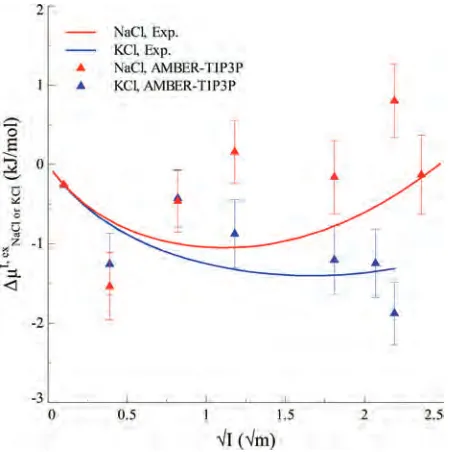
∆µI, exKCl and∆µNaClI, exusing the newly developed AMBER-TIP3P

force field26reproduces quantitatively the experimental data

(Figure 1), as previously reported.73,74 The CHARMM-TIP3P and Dang95-SPC/E force field-based calculations predict accurately the values for the KCl and NaCl solutions, respectively (Figure 2). All the other potential models are not as good (Figure 2). It is of interest to notice that a recent study75_{showed that the CHARMM parameters for Na-Cl}

interactions generated from the Lorentz-Berthelot combina-tion rule lead to a larger underestimacombina-tion of osmotic pressuresa probe for ions activitys12than the corresponding

one for K-Cl interactions.

3.2. Calculation of ∆µXI, ex. The calculated values for individual ions ∆µXI, ex (X ) Na

+

, K+, and Cl-) are as scattered at finite I as the corresponding ones for the KCl

Table 1. L-J Parameters of Ion Models and the Mixing Rules

model atom σ(nm) ε(kJ/mol) q (e) mixing rule

Na+ 0.21595 1.47545 1.0 AMBER26_{(SPC/E) K}+

0.28384 1.79789 1.0 Lorentz-Berthelot Cl- 0.48305 0.05349 -1.0

Na+ 0.24393 0.36585 1.0 AMBER26_{(TIP3P) K}+

0.30380 0.81041 1.0 Lorentz-Berthelot Cl- 0.44776 0.14891 -1.0

Na+ 0.24299 0.19623 1.0 CHARMM27,28 _K+

0.31426 0.36401 1.0 Lorentz-Berthelot Cl- 0.40447 0.62760 -1.0

Na+ 0.33304 0.01160 1.0

OPLS29 _K+

0.49346 0.00137 1.0 geometric Cl- 0.44172 0.49283 -1.0

Na+ 0.25840 0.41840 1.0 Dang9530 _K+

0.33320 0.41840 1.0 Lorentz-Berthelot Cl- 0.44010 0.41840 -1.0

SPC/E31 _{O 0.31660 0.65060 -0.8476}

H 0.00 0.00 0.4238

TIP3P32 _{O 0.31510 0.63640 -0.834}

H 0.00 0.00 0.417

H59,60 _{0.04000 0.19246 0.417}

Table 2. Numbers of Water Nwaterand Ion Pairs Nion pairin the Simulation System

ionic strength (m)

0.01 0.15 0.67 1.39 3.27 4.28 4.80 5.56 Nwater68 7804 7764 7624 7436 6986 6766 6656 6504 Nion pair 0 20 90 184 409 519 574 650

Figure 1. Calculated excess (electro-)chemical potential

differences for KCl∆µI, exKCl and NaCl∆µI, exNaCl, based on the newly developed AMBER-TIP3P force field,26_{plotted as a function}

and NaCl salts (Figure 3). This hints that thermodynamics of ions using different force fields differ from each other at finite I.

The magnitude of these values for ∆µXI, exis comparable

with that of the available experimentally derived data.24 However, the calculated∆µKI, ex+ increases with I more than

∆µNaI, ex+. The opposite trend is found in the experimental

estimates.76Similarly, the calculated∆µClI, ex- decreases with I more in the KCl solution than it does in the NaCl solution.

The opposite occurs for the experimentally derived values. These significant discrepancies may arise from several errors and assumptions from both theory and experiments, as discussed in the Introduction Section.

To provide some hints of the origin of errors specific to the calculations, we focus here on comparisons against results obtained using higher level calculations. These are available only for the electrical contribution zF(φI-φ°).

3.3. Some Considerations on the Electrical Contri-bution zF(φI-φ°). In this section, we report our calculated

values for zF(φI-φ°) at finite I and compare with previous calculations, based on polarizable force fields.48,49 Notice that also the latter results, even though they are expected to be much more accurate than those based on a nonpolarizable force field, still cannot present the exact Galvani potential. This is because they do not fully take into account the contribution due to the molecular quadrupoles.36,37

The calculated electrical contribution zF(φI - φ°) to

∆µKI, ex+ increases linearly with I for all the force fields used

here, ranging from 0 to 16 kJ/mol (Figure 4).77,78The range of the calculated values of zF(φI - φ°) is comparable to that obtained by polarizable ion/water force field-based calculations at I ) 1 m (from 1 to 4 kJ/mol versus 3.4 kJ/mol).48,79

The overall values of calculated zF(φI-φ°) for a Na+ range is from-3 to 3 kJ/mol. Thus, the values of zF(φI -φ°) at I)1 m range from-1 to 0.5 kJ/mol, to be compared with the value obtained with a polarizable force field of 3.5 kJ/mol.49,79We conclude that nonpolarizable models for the NaCl solution are not able to reproduce the results of polarizable models.

The experiments estimated an increase of the Galvani potential in both KCl and NaCl electrolyte solutions at finite I.37,80,81However the quantities are all much smaller (about

Figure 2. Deviationsεof calculated excess (electro-)chemical potential differences for KCl ∆µKClI, ex and NaCl ∆µNaClI, ex from experimental data34 _{plotted as a function of the m ionic}

strength. The shadow area covers the deviationεwithin(0.5 kJ/mol. The results obtained with all the force fields considered in this work are presented.

Figure 3. Calculated excess (electro-)chemical potential

differences for single ions∆µXI, ex(X)Na

+

, K+, and Cl-) in KCl and NaCl solutions, plotted as a function of the m ionic strength. The results obtained with all the force fields con-sidered in this work are presented. Experimentally derived estimates are also reported.24

Figure 4. Calculated electrical contribution zF(φI- φ°) to ∆µXI, exfor K

+

0.2 and 0.3 kJ/mol for KCl80,82and NaCl, respectively, at I ) _{1 m).}80,82

The very large discrepancies between theory and experiment reflect the difficulties in experimental measurement of the Galvani potential (see Introduction Section) as well as limitations of the molecular simulation methods outlined in the Introduction.

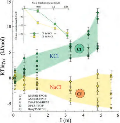
3.4. RT lnγCl-: Dependence from the Types of Coun-terions. The chemical contribution RT lnγCl-as a function

of I depends on the type of counterion for all the force fields used here (Figure 5).

As mentioned before, RT lnγCl- reflects the change of

intermolecular interactions between Cl--ion and Cl--water at finite I. This change in electrolyte solution is often attributed to the electrostatic interactions as a first ap-proximation.83We find the Cl--ion electrostatic contribution to RT lnγX of the NaCl solution is dramatically different

from that of the KCl solution, obtained from a calculation based on the newly developed AMBER-SPC/E force field26,84 (inset in Figure 5). Similar conclusions can be drawn for Cl--water electrostatic contributions in the two salt solutions (data not shown).

4. Implication for Biological Systems

The success of predicting the values for salts is gratifying with some of the force fields considered here, especially considering their very simple functional form. The success testifies to the care with which force fields have been developed. However, the challenges reported previously,13,20-22,55,85and addressed here, do remain in the prediction of∆µXI, ex(X)Na

+

, K+, and Cl-) and in particular of the electric contribution to it (see Sections 2.3 and 3.3). These difficulties may be even larger when modeling biological systems. Such difficulties do not come without consequence. Consider the simple identification of an ion channel, as done by (literally) thousands of laboratories

every day. That identification depends on the measurement and identity of the (so-called) reversal potential,86,87 which is the experimental estimator of the gradient of chemical potential or the equilibrium potential, as it was called by Hodgkin and Huxley.88,89The name of the channel is often determined by its selectivity90-93(e.g., sodium, potassium, or chloride chan-nels), and that in turn depends on the identification of the reversal potential with the gradient of chemical potential of one ion. If in fact ∆µXI, ex is not accurately included94

-98

in the calculation of the gradient of chemical potential (when using concentration of ions as inputs), then the channel identification may be askew.97

The selectivity properties of ion channels are crucially important to their function. Ions that differ in their nonideal properties, like Na+and K+, carry different ‘messages’ (i.e., signals) to different systems of the cell, and so there is enormous literature trying to measure, understand, simulate, control, and even synthesize99-101 the selectivity of different types of channels. Estimates and computations of selectivity depend critically on estimates of∆µXI, ex, because many types of ions

differ only because they are nonideal. Similar considera-tions87,102-113are likely to apply to a myriad of other biological events. Many important biological properties arise because of the nonideal properties of individual types of ions.

5. Conclusion

We have established the quality of a variety of standard ion/ water force fields commonly used in biological simulation, for the calculation of the excess (electro-)chemical potential for KCl

∆µKClI, exand for NaCl∆µNaClI, ex. Specifically, the AMBER26(the

newly developed), CHARMM,27,28 OPLS,29 and Dang9530 were considered in combination with SPC/E31 and TIP3P32 water models. The calculation based on the newly developed AMBER-TIP3P agrees well with the experimental values for both KCl and NaCl solutions, as previously reported.73Instead the CHARMM-TIP3P potential agrees well with the KCl salt, whereas the Dang95-SPC/E potential agrees well with the NaCl salt. The other potential models do not give good results for either of the two aqueous solutions studied. Hence, care should be taken in biomolecular simulations when using these force fields at physiological I.

The calculated∆µNaI, ex+ values are similar to those of∆µKI, ex+ .

The calculated values are as scattered at finite I as the corresponding ones for the KCl and NaCl salts. Only the calculated electric contribution zF(φI-φ°) of K+is consistent with reported higher level calculations with polarizable ion/ water force fields.48

The calculated chemical contribution RT lnγCl-to∆µClI, ex

-depends on the type of counterions present. This result may be of interest for force field calculations of Cl--dependent biological systems (such as chloride channels).114

Acknowledgment. The author (C. Z.) thanks F. Marinel-li for helpful discussion on the repMarinel-lica-exchange method. We thank the reviewers for their highly valuable comments on the manuscript.

Supporting Information Available: Tests of the convergence of free-energy calculation, calculated dielectric constants as a function of ionic strength, estimates of the

Galvani potential of pure water as well as the density profiles of concentrated salt solutions. This material is available free of charge via the Internet at http://pubs.acs.org.

References

(1) “m” is molal scale not molar scale, i.e., m is mol/1 kg of H2O.

(2) Costanzo, L. S.Physiology; Elsevier/Saunders: Philadelphia, PA, 2006; pp 2-4.

(3) Gouaux, E.; MacKinnon, R.Science2005, 310, 1461.

(4) Doyle, D. A.; Cabral, J. M.; Pfuetzner, R. A.; Kuo, A.; Gulbis, J. M.; Cohen, S. L.; Chait, B. T.; MacKinnon, R.

Science1998, 280, 69.

(5) Domene, C.; Vemparala, S.; Furini, S.; Sharp, K.; Klein, M. L.J. Am. Chem. Soc.2008, 130, 11.

(6) Jayaram, B.; Jain, T.Annu. ReV. Biophys. Biomol. Struct. 2004, 33, 343.

(7) Auffinger, P.; Hashem, Y.Curr. Opin. Struct. Biol.2007,

17, 325.

(8) Chu, V. B.; Bai, Y.; Lipfert, J.; Herschlag, D.; Doniach, S.

Curr. Opin. Chem. Biol.2008, 12, 619.

(9) Lee, L. L. Molecular Thermodynamics of Electrolyte Solutions; World Scientific: New York, 2008; pp 11-38.

(10) Beck, T. L.; Paulaitis, M. E.; Pratt, L. R. The Potential Distribution Theorem and Models of Molecular Solutions; Cambridge University Press: Cambridge, U.K., 2006; pp 45 -68.

(11) Butt, H. J.; Graf, K.; Kappl, M.Physics and Chemistry of Interfaces; Wiley-VCH: Weinheim, Germany, 2006; pp 77 -79.

(12) Liquids, Solutions, and Interfaces: From Classical Mac-roscopic Descriptions to Modern MicMac-roscopic Details; Fawcett, W. R., Ed.; Oxford University Press: New York, 2004; pp 3-147.

(13) Kastenholz, M. A.; Hnenberger, P. H.J. Chem. Phys.2006,

124, 224501.

(14) Lamoureux, G.; Roux, R.J. Phys. Chem. B2006, 110, 3308.

(15) van Gunsteren, W. F.; et al.Angew. Chem., Int. Ed.2006,

45, 4064.

(16) McDowell, S. E.; Spackova, N.; Sponer, J.; Walter, N. G.

Biopolymer2007, 82, 169.

(17) Hummer, G.; Pratt, L. R.; Garcı´a, A. E.J. Phys. Chem.1996,

100, 1206.

(18) Hummer, G.; Pratt, L. R.; Garca´, A. E.J. Chem. Phys.1997,

107, 9275.

(19) Hu¨nenberger, P. H.; McCammon, J. A.J. Chem. Phys.1999,

110, 1856.

(20) Conway, B. E.J. Sol. Chem.1978, 7, 720–770.

(21) Marcus, Y.J. Chem. Soc. Faraday Trans.1987, 83, 2985.

(22) Tissandier, M. D.; Cowen, K. A.; Feng, W. Y.; Gundlach, E.; Cohen, M. H.; Earhart, A. D.; Coe, J. V.J. Phys. Chem. A1998, 102, 7787.

(23) Fawcett, W. R.Langmuir2008, 24, 9868.

(24) Wilczek-Vera, G.; Rodil, E.; Vera, J. H.AIChE J. 2004,

50, 445.

(25) Within these simplifying assumptions, the Galvani potential is the same for K+and Na+, and it is opposite in sign for Cl-.

(26) Joung, I. S.; Cheatham, T. E., IIIJ. Phys. Chem. B2008,

112, 9020.

(27) Beglov, D.; Roux, B.J. Chem. Phys.1994, 100, 9050.

(28) Roux, B.Biophys. J.1996, 71, 3177.

(29) Jorgensen, W. L.; Maxwell, D. S.; Tirado-Rives, J.J. Am. Chem. Soc.1996, 118, 11225.

(30) Dang, L. X.J. Am. Chem. Soc.1995, 117, 6954.

(31) Berendsen, H. J. C.; Grigera, J. R.; Straatsma, T. P.J. Phys. Chem.1987, 91, 6269.

(32) Jorgensen, W. L.; Chandrasekhar, J.; Madura, J. D.; Impey, R. W.; Klein, M. L.J. Chem. Phys.1983, 79, 926.

(33) Patra, M.; Karttunen, M.J. Comput. Chem.2004, 25, 678.

(34) Hamer, W. J.; Wu, Y.-C.J. Phys. Chem. Ref. Data1972,

1, 1047.

(35) Fawcett, W. R.Liquids, Solutions, and Interfaces: From Classical Macroscopic Descriptions to Modern Micro-scopic Details; Oxford University Press: New York, 2004; pp 395-422.

(36) Paluch, M.AdV. Colloid Interface Sci.2000, 84, 27.

(37) Petersen, P. B.; Saykally, R. J. Annu. ReV. Phys. Chem. 2006, 57, 333.

(38) Continuum models encounter difficulties in describing the Galvani potential because the latter depends on the polariza-tion of the system.

(39) Kirkwood, J. G.J. Chem. Phys.1935, 3, 300.

(40) Ferrrario, M.; Ciccoti, G.; Spohr, E.; Cartailler, T.; Turq, P.

J. Chem. Phys.2002, 117, 4947.

(41) Free Energy Calculations; Chipot, C., Pohorille, A., Eds.; Springer-Verlag: Berlin, Germany, 2007; pp 33-72.

(42) Fukunishi, H.; Watanabe, O.; Takada, S.J. Chem. Phys. 2002, 116, 9058.

(43) Woods, C. J.; Essex, J. W.; King, M. A.J. Phys. Chem B 2003, 107, 13711.

(44) Jiang, W.; Hodoscek, M.; Roux, B. J. Chem. Theory Comput.2009, 5, 2583.

(45) Uchida, H.; Matsuoka, M.Fluid Phase Equilib.2004, 219, 49.

(46) Chowdhuri, S.; Chandra, A.J. Chem. Phys.2001, 115, 3732.

(47) Instead, the diffusion of ions has no impact on the conver-gence of TI calculation at infinite dilution.

(48) Wick, C. D.; Dang, L. X.; Jungwirth, P.J. Chem. Phys. 2006, 125, 024706.

(49) Bauer, B. A.; Patel, S.J. Chem. Phys.2010, 132, 024713.

(50) Kastenholz, M. A.; Hu¨nenberger, P. H.J. Chem. Phys.2006,

124, 124106.

(51) Sagul, C.; Darden, T. A. Annu. ReV. Biophys. Biomol. Struct.1999, 28, 155.

(52) Feller, S. E.; Pastor, R. W.; Rojnuckarin, A.; Bogusz, S.; Brooks, B. R.J. Phys. Chem.1996, 100, 17011.

(53) Sokhan, V. P.; Tildesley, D. J.Mol. Phys.1997, 92, 625.

(55) Cheng, J.; Sulpizi, M.; Sprik, M.J. Chem. Phys.2009, 131, 154504.

(56) The calculated static dielectric constants ε(0) of KCl and NaCl solutions comparing with experimental data as a function of the molal ionic strength can be seen in Supporting Information, Figure S2.

(57) van der Spoel, D.; Lindahl, E.; Hess, B.; Groenhof, G.; Mark, A. E.; Berendsen, H. J. C.J. Comput. Chem.2005, 26, 1701.

(58) Hess, B.; Kutzner, C.; van der Spoel, D.; Lindahl, E.

J. Chem. Theory Comput.2008, 4, 435.

(59) MacKerell, A. D., Jr.; et al.J. Phys. Chem. B1998, 102, 3586.

(60) Modified TIP3P water in CHARMM59 .

(61) Lin, Y.; Baumketner, A.; Deng, S.; Xu, Z.; Jacobs, D.; Cai, W.J. Chem. Phys.2009, 131, 154103.

(62) Nos´e, S.J. Chem. Phys.1984, 81, 511.

(63) Hoover, W. G.Phys. ReV. A: At., Mol., Opt. Phys.1985,

31, 1695.

(64) Parrinello, M.; Rahman, A.Phys. ReV. Lett.1980, 45, 1196.

(65) Essmann, U.; Perera, L.; Berkowitz, M. L.; Darden, T.; Lee, H.; Pedersen, L. G.J. Chem. Phys.1995, 103, 8577.

(66) Allen, M. P.; Tildesley, D. J. Computer Simulation of Liquids: Oxford Science Publications: Oxford, U.K., 1987; pp 64-68.

(67) Miyamoto, S.; Kollman, P. A.J. Comput. Chem.1992, 13, 952.

(68) Exact number depends on the water model and the salt type.

(69) Kollman, P.Chem. ReV.1993, 93, 2395.

(70) Beutler, T. C.; Mark, A. E.; Van Schaik, R. C.; Gerber, P. R.; Van Gunsteren, W. F.Chem. Phys. Lett.1994, 222, 529.

(71) Hess, B.J. Chem. Phys.2002, 116, 209.

(72) Note that it is also possible to obtain the Galvani potential by creating a virtual air-solution interface with those snapshots from simulations of bulk solutions under PBC and then integrating the charge density.

(73) Joung, I. S.; Cheatham, T. E.J. Phys. Chem. B2009, 113, 13279.

(74) Notice that the time-scale of our simulation is shorter than that of these authors.73

They use straightforward TI instead of replica-exchange TI. The latter converges faster, See Figure S1 in Supporting Information..

(75) Luo, Y.; Roux, B.J. Phys. Chem. Lett. 2010, 1, 183.

(76) Similar trends were also founded experimentally24 in the presence of an anion other than Cl-.

(77) Table S1 in Supporting Information presents a comparison ofφ°values, which is not crucial for the∆µXI, exbut may be

relevant as a reference.

(78) We only observed a slight preference of the anions at the interface than cations in the simulations (See Figure S3 in Supporting Information).

(79) The actual values reported in refs48 and 49 are (φI

-φ°). For the sake of clarity, here we report zF(φI

-φ°), which is the quantity of interest here.

(80) Randles, J. E.Phys. Chem. Liq.1977, 7, 107.

(81) Jungwirth, P.; Tobias, D. J.Chem. ReV.2006, 106, 1259.

(82) Jarvis, N. J.; Scheiman, M. A. J. Phys. Chem.1968, 72, 74.

(83) Wright, M. R. An Introduction to Aqueous Electrolyte Solutions; Wiley: Chichester, U.K., 2007.

(84) We expect similar results for all the other force fields as they have the same trend in Figure 5. However, free energy decomposition is force field and path dependent.

(85) Harder, E.; Roux, B.J. Chem. Phys. 2008, 129, 234706.

(86) Hille, B.Ionic Channels of Excitable Membranes, 3rd ed.; Sinauer Associates Inc.: Sunderland, MA, 2001; pp 1-19.

(87) Zuhlke, R. D.; Pitt, G. S.; Deisseroth, K.; Tsien, R. W.; Reuter, H.Nature1999, 399, 159.

(88) Hodgkin, A.; Huxley, A.; Katz, B.Arch. Sci. Physiol.1949,

3, 129.

(89) Hodgkin, A.J. Physiol.1976, 263, 1.

(90) Conley, E. C.The Ion Channel Facts Book. I. Extracellular Ligand-gated Channels; Academic Press: New York, 1996; pp 3-11.

(91) Conley, E. C.The Ion Channel Facts Book. II. Intracellular Ligand-gated Channels; Academic Press: New York, 1996; pp 3-20.

(92) Conley, E. C.; Brammar, W.The Ion Channel Facts Book III: Inward Rectifier and Intercellular Channels; Academic Press: New York2000; pp 3-21.

(93) Conley, E. C.; Brammar, W.The Ion Channel Facts Book IV: Voltage Gated Channels; Academic Press: New York, 1999; pp 3-21.

(94) Barry, P. H.Am. J. Physiol.1990, 259, S15.

(95) Barry, P. H.Ann. Biomed. Eng.1994, 22, 218.

(96) Barry, P. H.J. Neurosci. Methods1994, 51, 107.

(97) Barry, P. H.Cell Biochem. Biophys.2006, 46, 143.

(98) Ng, B.; Barry, P. H.J. Neurosci. Methods 1995, 56, 37.

(99) Miedema, H.; Meter-Arkema, A.; Wieregna, J.; Tang, J.; Eisenberg, B.; Nonner, W.; Hektor, H.; Gillespie, D.; Meijberg, W.Biophys. J.2004, 87, 3137.

(100) Miedema, H.; Vrouenraets, M.; Wieregna, J.; Eisenberg, B.; Gillespie, D.; Meijberg, W.; Nonner, W.Biophys. J.2006,

91, 4392.

(101) Vrouenraets, M.; Wieregna, J.; Meijberg, W.; Miedema, H.

Biophys. J.2006, 90, 1202.

(102) Berg, J. M. Annu. ReV. Biophys. Biophys. Chem. 1990,

19, 405.

(103) Berg, J. M.J. Biol. Chem.1990, 265, 6513.

(104) Cantwell, M. A.; Di Cera, E. J. Biol. Chem.2000, 275, 39827.

(105) Berg, J. M.; Godwin, H. A.Annu. ReV. Biophys. Biomol. Struct.1997, 26, 357.

(106) Carnell, C. J.; Bush, L. A.; Mathews, F. S.; Di Cera, E.

Biophys. Chem.2006, 121, 177.

(107) De Gristofaro, R.; Fenton II, J. W.; Di Cera, E.J. Mol. Biol. 1992, 226, 263.

(108) Di Cera, E.Biopolymer1994, 34, 1001.

(109) Doroshenko, P. A.; Kostyuk, P. G.; Lukyanetz, E. A.

Neurosci.1998, 27, 1073.

(111) Lambers, T. T.; Mahieu, F.; Oancea, E.; Hoofd, L.; de Lange, F.; Mensenkamp, A. R.; Voets, T.; Nilinus, B.; Clapham, D. E.; Hoenderop, J. G.; Bindels, R. J.EMBO J.2006, 25, 2978.

(112) Tripathy, A.; Xu, L.; Mann, G.; Meissner, G.Biophys. J. 1995, 69, 106.

(113) Vescovi, E. G.; Ayala, Y. M.; Di Cera, E.; Groisman, E. A.

J. Biol. Chem.1997, 272, 1440.

(114) Suzuki, M.; Morita, T.; Iwamoto, T. Cell. Mol. Life Sci. 2006, 63, 12.

Supporting Information

Chao Zhang, Simone Raugei, Bob Eisenberg, Paolo Carloni

German Research School for Simulation Sciences, FZ-Juelich/RWTH Aachen University, Germany; Statistical and Biological Physics sector, SISSA, Italy;

Rush University Medical Center, Chicago, IL

A

Convergence of free-energy calculation

The convergence of the free-energy estimate was tested running simulations starting from differ-ent (uncorrelated) configurations, using differdiffer-ent numbers ofλwindows and different sampling times. Specifically,­UI®LJ_I,λand­UI®Q_I,λcontributions to free energy have been calculated us-ing straightforward TI and its replica-exchange variant. For sake of simplicity, in the followus-ing only the results obtained for the newly developed AMBER-SPC/E potential [1] are discussed. Similar features are expected for the other force-fields.

As can be seen from Figure S1 (bottom, left panel), when using replica-exchange TI, the term ­UI®LJ_I,λ turns out not to depend significantly on the initial configuration. Conversely, using straightforward TI results strongly depend on the initial configuration (Figure S1 (top, left panel). Similar conclusions are obtained for the term ­UI®Q_I,λ (Data not shown). As a

whole, the final free energy difference− 1 βln

R1

0 dλ

­

UI®_I,λ can change as much as 5 kJ/mol changing the starting point of simulations using straightforward TI.

The dependence of the average from the number ofλwindows is reported in Figure S1 (right panel) for the term­

UI®Q

I,λ. We remark that this is the larger of the two contributions to the thermodynamic force­UI®_I,λ. As can be seen, 10λwindows are sufficient to have converged values using with replica-exchange TI. The same is not likely to be true for the straightforward TI.

B

Dielectric constants of ionic solutions

See Figure S2.

C

Estimates of the Galvani potential of pure water

See Table S1.

D

Density profiles of concentrated salt aqueous solutions

See Figure S3. Similar results apply for other force-fields used in the text (Data not shown).

0 0.1 0.2 0.3 0.4 0.5 0.6 0.7 0.8 0.9 1 −100

−80 −60 −40 −20

λ

<U

I>

LJ

I,

λ

(kJ/mol)

Straightforward TI

Config. 1 Config. 2 Config. 3

0 0.1 0.2 0.3 0.4 0.5 0.6 0.7 0.8 0.9 1 −100

−80 −60 −40 −20 0

λ

<U

I>

LJ

I,

λ

(kJ/mol)

Replica−exchange TI

Config. 1 Config. 2 Config. 3

0 0.05 0.1 0.15 0.2 0.25 0.3 0.35 0.4 0.45 0.5 400

450 500 550 600 650 700 750

λ

<U

I> QI,

λ

(kJ/mol)

Straightforward TI, 10 λ windows Replica−exchange TI, 10 λ windows Replica−exchange TI, 20 λ windows

Figure S1: Ensemble averages of the Lennard-Jones potential contribution,­UI®LJ_I,λ(left), and

the electrostatic interaction contribution,­UI®Q_I,λ(right), to the thermodynamic force­UI®_I,λ

for the KCl solution at 3.27m calculated for the newly developed AMBER-SPC/E potential [1]. Each contribution is calculated with both straightforward TI and replica-exchange TI, plotted as function of the coupling parameterλ. Comparison between different initial configurations and different numbers ofλwindows is made for­

UI®LJ

I,λ and

­

UI®Q

I,λ, respectively. In each point, the average is calculated over a 200 ps trajectory.

0 1 2 3 4 5 6

20 30 40 50 60 70 80 90 100 110 120

I (m)

ε

(0)

KCl

Exp. AMBER−SPC/E AMBER−TIP3P CHARMM−TIP3P OPLS−TIP3P Dang95−SPC/E

0 1 2 3 4 5 6

20 30 40 50 60 70 80 90 100 110 120

I (m)

ε

(0)

NaCl

Exp. AMBER−SPC/E AMBER−TIP3P CHARMM−TIP3P OPLS−TIP3P Dang95−SPC/E

Figure S2: Calculated and experimental [2] static dielectric constantǫ(0)as a function of the molal ionic strengthI for KCl and NaCl aqueous solutions.

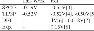
Table S1: Estimates of the Galvani potential of pure liquid waterϕ◦_{at 298 K. Results obtained}

in the present work are compared with previous calculations and experimental-derived values. This Work Ref.

SPC/E -0.59V -0.55V[3]

TIP3P -0.52V -0.52V[4], -0.50V[5]

DFT – 4V[6], -0.018V[7]

Exp. – 0.15V[8]

References

[1] I. S. Joung and T. E. Cheatham, III. Determination of alkali and halide monovalent ion parameters for use in explicitly solvated biomolecular simulations. J. Phys. Chem. B,

S

R-ScP5R-S/ E

R-ScP5R-S/

-A

/

gM

+ +P+3 +Pρ +Pρ3 +P(

-AƿM

c cP3 3 3P3 )

R

E-RcS3E-RP B

E-RcS3E-RP

-m

P

(A

/ /S/c /S+ /S+c /Sρ

-mƿA

g gSc c cSc 3

Figure S3: Density profiles for K+ and Cl− _{ions in KCl solution at 4.8 m and for Na}+ _and

Cl−_{ions in NaCl solution at 5.6 m calculated with the newly developed AMBER-SPC/E}

poten-tial [1].

112:9020–9041, 2008.

[2] J. Barthel, R. Buchner, and M. M¨unsterer. Electrolyte Date Collection, Part2: Dielectric

Properties of Water and Aqueous Electrolyte Solutions. Dechema: Frankfurt, 1995.

[3] V. P. Sokhan and D. J. Tildesley. The free surface of water: molecular orientation, surface potential and nonlinear susceptibility. Mol. Phys., 92:625–640, 1997.

[4] E. Harder and B. Roux. On the origin of the electrostatic potential difference at a liquid-vacuum interface. J. Chem. Phys., 129:234706, 2008.

[5] S. E. Feller, R. W. Pastor, A. Rojnuckarin, S. Bogusz, and B. R. Brooks. Effect of elec-trostatic force truncation on interfacial and transport properties of water. J. Phys. Chem., 100:17011–17020, 1996.

[6] P. Hunt and M. Sprik. On the position of the highest occupied molecular orbital in aqueous solutions of simple ions. ChemPhysChem, 6:1805–1808, 2005.

[7] S. M. Kathmann, I-F. W. Kuo, and C. Mundy. Electronic effects on the surface potential at the vapor-liquid interface of water. J. Am. Chem. Soc., 130:16556–16561, 2008.

[8] W. R. Fawcett. The ionic work function and its role in estimating absolute electrode poten-tials. Langmuir, 24:9868–9875, 2008.