Explaining Recurrent Neural Network Predictions in Sentiment Analysis
Leila Arras1, Gr´egoire Montavon2, Klaus-Robert M¨uller2,3,4, and Wojciech Samek1 1Machine Learning Group, Fraunhofer Heinrich Hertz Institute, Berlin, Germany
2Machine Learning Group, Technische Universit¨at Berlin, Berlin, Germany 3Department of Brain and Cognitive Engineering, Korea University, Seoul, Korea
4Max Planck Institute for Informatics, Saarbr¨ucken, Germany
{leila.arras, wojciech.samek}@hhi.fraunhofer.de
Abstract
Recently, a technique called Layer-wise Relevance Propagation (LRP) was shown to deliver insightful explanations in the form of input space relevances for un-derstanding feed-forward neural network classification decisions. In the present work, we extend the usage of LRP to recurrent neural networks. We propose a specific propagation rule applicable to multiplicative connections as they arise in recurrent network architectures such as LSTMs and GRUs. We apply our technique to a word-based bi-directional LSTM model on a five-class sentiment prediction task, and evaluate the result-ing LRP relevances both qualitatively and quantitatively, obtaining better results than a gradient-based related method which was used in previous work.
1 Introduction
Semantic composition plays an important role in sentiment analysis of phrases and sentences. This includes detecting the scope and impact of nega-tion in reversing a sentiment’s polarity, as well as quantifying the influence of modifiers, such as de-gree adverbs and intensifiers, in rescaling the sen-timent’s intensity (Mohammad,2017).
Recently, a trend emerged for tackling these challenges via deep learning models such as con-volutional and recurrent neural networks, as ob-served e.g. on the SemEval-2016 Task for Senti-ment Analysis in Twitter(Nakov et al.,2016).
As these models become increasingly predic-tive, one also needs to make sure that they work as intended, in particular, their decisions should be made as transparent as possible.
Some forms of transparency are readily ob-tained from the structure of the model, e.g. re-cursive nets (Socher et al.,2013), where sentiment can be probed at each node of a parsing tree.
Another type of analysis seeks to determine what input features were important for reaching the final top-layer prediction. Recent work in this direction has focused on bringing measures of feature importance to state-of-the-art models such as deep convolutional neural networks for vision (Simonyan et al., 2014; Zeiler and Fergus, 2014;
Bach et al.,2015;Ribeiro et al.,2016), or to gen-eral deep neural networks for text (Denil et al.,
2014;Li et al.,2016a;Arras et al.,2016a;Li et al.,
2016b;Murdoch and Szlam,2017).
Some of these techniques are based on the model’s local gradient information while other methods seek to redistribute the function’s value on the input variables, typically by reverse prop-agation in the neural network graph (Landecker et al., 2013; Bach et al., 2015; Montavon et al.,
2017a). We refer the reader to (Montavon et al.,
2017b) for an overview on methods for under-standing and interpreting deep neural network pre-dictions.
Bach et al. (2015) proposed specific propaga-tion rules for neural networks (LRP rules). These rules were shown to produce better explanations than e.g. gradient-based techniques (Samek et al.,
2017), and were also successfully transferred to neural networks for text data (Arras et al.,2016b). In this paper, we extend LRP with a rule that handles multiplicative interactions in the LSTM model, a particularly suitable model for modeling long-range interactions in texts such as those oc-curring in sentiment analysis.
We then apply the extended LRP method to a bi-directional LSTM trained on a five-class sentiment prediction task. It allows us to produce reliable explanations of which words are responsible for
attributing sentiment in individual texts, compared to the explanations obtained by using a gradient-based approach.
2 Methods
Given a trained neural network that models a scalar-valued prediction function fc (also
com-monly referred to as a prediction score) for each class c of a classification problem, and given an input vectorx, we are interested in computing for each input dimensiondofxa relevance scoreRd
quantifying the relevance of xd w.r.t to a
consid-ered target class of interest c. In others words, we want to analyze which features ofxare impor-tant for the classifier’s decisiontowardoragainst
a classc.
In order to estimate the relevance of a pool of input space dimensions or variables (e.g. in NLP, when using distributed word embeddings as input, we would like to compute the relevance of a word, and not just of its single vector dimensions), we simply sum up the relevance scoresRdof its
con-stituting dimensionsd.
In this described framework, there are two alter-native methods to obtain the single input variable’s relevance in the first place, which we detail in the following subsections.
2.1 Gradient-based Sensitivity Analysis (SA)
The relevances can be obtained by computing squared partial derivatives:
Rd=
∂fc
∂xd(x)
2
.
For a neural network classifier, these derivatives can be obtained by standard gradient backprop-agation (Rumelhart et al., 1986), and are made available by most neural network toolboxes. We refer to the above definition of relevance as Sen-sitivity Analysis (SA) (Dimopoulos et al., 1995;
Gevrey et al., 2003). A similar technique was previously used in computer vision by (Simonyan et al.,2014), and in NLP by (Li et al.,2016a).
Note that if we sum up the relevances of all in-put space dimensions d, we obtain the quantity
k∇x fc(x)k22, thus SA can be interpreted as a
de-composition of the squared gradient norm.
2.2 Layer-wise Relevance Propagation (LRP)
Another technique to compute relevances was pro-posed in (Bach et al.,2015) as the Layer-wise Rel-evance Propagation (LRP) algorithm. It is based
on a layer-wise relevance conservation principle, and, for a given inputx, it redistributes the quan-tityfc(x), starting from the output layer of the
net-work and backpropagating this quantity up to the input layer. The LRP relevance propagation proce-dure can be described layer-by-layer for each type of layer occurring in a deep convolutional neu-ral network (weighted linear connections follow-ing non-linear activation, poolfollow-ing, normalization), and consists in defining rules for attributing rele-vance to lower-layer neurons given the relerele-vances of upper-layer neurons. Hereby each intermediate layer neuron gets attributed a relevance score, up to the input layer neurons.
In the case of recurrent neural network architec-tures such as LSTMs (Hochreiter and Schmidhu-ber,1997) and GRUs (Cho et al.,2014), there are two types of neural connections involved: many-to-one weighted linear connections, and two-to-one multiplicative interactions. Hence, we restrict our definition of the LRP procedure to these types of connections. Note that, for simplification, we refrain from explicitly introducing a notation for non-linear activation functions; if such an activa-tion is present at a neuron, we always take into account the activated lower-layer neuron’s value in the subsequent formulas.
In order to compute the input space relevances, we start by setting the relevance of the output layer neuron corresponding to the target class of interest
cto the value fc(x), and simply ignore the other
output layer neurons (or equivalently set their rele-vance to zero). Then, we compute layer-by-layer a relevance score for each intermediate lower-layer neuron accordingly to one of the subsequent for-mulas, depending on the type of connection in-volved.
Weighted Connections. Letzj be an upper-layer
neuron, whose value in the forward pass is com-puted aszj = Pizi ·wij +bj, wherezi are the
lower-layer neurons, and wij, bj are the
connec-tion weights and biases.
Given the relevancesRjof the upper-layer
neu-rons zj, the goal is to compute the lower-layer
relevances Ri of the neurons zi. (In the
partic-ular case of the output layer, we have a single upper-layer neuron zj, whose relevance is set to
its value, more precisely we set Rj = fc(x) to
Ri←j going from upper-layer neuronszjto
lower-layer neuronszi. Then, by summing up incoming
messages for each lower-layer neuronzito obtain
the relevance Ri. The messages Ri←j are
com-puted as a fraction of the relevanceRjaccordingly
to the following rule:
Ri←j = zi·wij +
·sign(zj) +δ·bj
N
zj+·sign(zj) ·Rj
where N is the total number of lower-layer neu-rons to which zj is connected, is a small
posi-tive number which serves as a stabilizer (we use
= 0.001in our experiments), and sign(zj) =
(1zj≥0 −1zj<0) is defined as the sign ofzj. The
relevance Ri is subsequently computed as Ri =
P
jRi←j. Moreover,δ is a multiplicative factor
that is either set to 1.0, in which case the total relevance of all neurons in the same layer is con-served, or else it is set to 0.0, which implies that a part of the total relevance is “absorbed” by the bi-ases and that the relevance propagation rule is ap-proximately conservative. Per default we use the last variant withδ = 0.0 when we refer to LRP, and denote explicitly by LRPconsour results when
we useδ = 1.0in our experiments.
Multiplicative Interactions. Another type of connection is a two-way multiplicative interaction between lower-layer neurons. Letzj be an
upper-layer neuron, whose value in the forward pass is computed as the multiplication of the two lower-layer neuron valueszg and zs, i.e. zj = zg ·zs.
In such multiplicative interactions, as they occur e.g. in LSTMs and GRUs, there is always one of the two lower-layer neurons that constitutes a
gate, and whose value ranges between[0,1]as the output of a sigmoid activation function (or in the particular case of GRUs, can also be equal to one minus a sigmoid activated value), we call it the
gateneuronzg, and refer to the remaining one as
thesourceneuronzs.
Given such a configuration, and denoting byRj
the relevance of the upper-layer neuronzj, we
pro-pose to redistribute the relevance onto lower-layer neurons in the following way: we setRg = 0and
Rs = Rj. The intuition behind this reallocation
rule, is that thegateneuron decides already in the forward pass how much of the information con-tained in thesource neuron should be retained to make the overall classification decision. Thereby the valuezg controls how much relevance will be
attributed to zj from upper-layer neurons. Thus,
even if our local propagation rule seems to ignore the respective values of zg andzs to redistribute
the relevance, these are indeed taken into account when computing the valueRjfrom the relevances
of thenextupper-layer neurons to whichzj is
con-nected via weighted connections.
3 Recurrent Model and Data
As a recurrent neural network model we em-ploy a one hidden-layer bi-directional LSTM (bi-LSTM), trained on five-class sentiment prediction of phrases and sentences on the Stanford Sen-timent Treebank movie reviews dataset (Socher et al., 2013), as was used in previous work on neural network interpretability (Li et al., 2016a) and made available by the authors1. This model
takes as input a sequence of words x1, x2, ..., xT
(as well as this sequence in reversed order), where each word is represented by a word embedding of dimension 60, and has a hidden layer size of 60. A thorough model description can be found in the Appendix, and for details on the training we refer to (Li et al.,2016a).
In our experiments, we use as input the 2210 to-kenized sentences of the Stanford Sentiment Tree-bank test set (Socher et al.,2013), preprocessing them by lowercasing as was done in (Li et al.,
2016a). On five-class sentiment prediction of full sentences (very negative, negative, neutral, posi-tive, very positive) the model achieves 46.3% ac-curacy, and for binary classification (positive vs. negative, ignoring neutral sentences) the test ac-curacy is 82.9%.
Using this trained bi-LSTM, we compare two relevance decomposition methods: sensitivity analysis (SA) and Layer-wise Relevance Propa-gation (LRP). The former is similar to the “First-Derivative Saliency” used in (Li et al.,2016a), be-sides that in their work the authors do not aggre-gate the relevance of single input variables to ob-tain a word-level relevance value (i.e. they only visualize relevance distributed over word embed-ding dimensions); moreover they employ the abso-lute value of partial derivatives (instead of squared partial derivatives as we do) to compute the rele-vance of single input variables.
In order to enable reproducibility and for en-couraging further research, we make our
imple-1https://github.com/jiweil/
mentation of both relevance decomposition meth-ods available2(see also (Lapuschkin et al.,2016)).
4 Results
In this Section, we present qualitative as well as quantitative results we obtained by performing SA and LRP on test set sentences. As an outcome of the relevance decomposition for a chosen tar-getclass, we first get for each word embeddingxt
in an input sentence, avectorof relevance values. In order to obtain a scalarword-level relevance, we remind that we simply sum up the relevances contained in that vector. Also note that, per def-inition, the SA relevances are positive while LRP relevances are signed.
4.1 Decomposing Sentiment onto Words
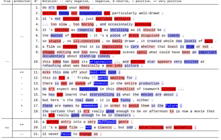
In order to illustrate the differences between SA and LRP, we provide in Fig. 1 and 2 heatmaps of exemplary test set sentences. These heatmaps were obtained by mapping positive word-level rel-evance values to red, and negative relrel-evances to blue. The exemplary sentences belong either to the class “very negative” or to the class “very pos-itive”, and the target class for relevance decom-position is always the true class. On the left of the Figures, we indicate the true sentence class, as well as the bi-LSTM’spredictedclass, whereby the upper examples are correctly classified while the bottom examples are falsely classified.
From the inspection of the heatmaps, we no-tice that SA does not clearly distinguish between words speakingfororagainstthe target class. In-deed it sometimes attributes a comparatively high relevance to words expressing a positive apprecia-tion likethrilling(example 5),master(example 6) ormust-see(example 11), while the target class is “very negative”; or to the worddifficult(example 19) expressing a negative judgment, while the tar-get class is “very positive”. On the contrary, LRP can discern more reliably between words address-ing a negative sentiment, such aswaste(1), horri-ble(3), disaster(6),repetitive(9) (highlighted in red), or difficult (19) (highlighted in blue), from words indicating a positive opinion, likefunny(2),
suspenseful (2), romantic (5), thrilling (5) (high-lighted in blue), orworthy(19),entertaining(20) (highlighted in red).
2https://github.com/ArrasL/LRP_for_
LSTM
Furthermore, LRP explains well the two sen-tences that are mistakenly classified as “very pos-itive” and “pospos-itive” (examples 11 and 17), by ac-centuating the negative relevance (blue colored) of terms speaking against the target class, i.e. the class “very negative”, such as must-see list, re-memberandfuture, whereas such understanding is not provided by the SA heatmaps. The same holds for the misclassified “very positive” sentence (ex-ample 21), where the word failsgets attributed a deep negatively signed relevance (blue colored). A similar limitation of gradient-based relevance visualization for explaining predictions of recur-rent models was also observed in previous work (Li et al.,2016a).
Moreover, an interesting property we observe with LRP, is that the sentiment of negation is mod-ulated by the sentiment of the subsequent words in the sentence. Hence, e.g. in the heatmaps for the target class “very negative”, when negators liken’t
or not are followed by words indicating a nega-tive sentiment likewaste(1) orhorrible(3), they are marked by a negatively signed relevance (blue colored), while when the subsequent words ex-press a positive imex-pression like worth (12), sur-prises (14), funny (16) or good (18), they get a positively signed relevance (red colored).
Thereby, the heatmap visualizations provide some insights on how the sentiment of single words is composed by the bi-LSTM model, and indicate that the sentiment attributed to words is not static, but depends on their context in the sen-tence. Nevertheless, we would like to point out that the explanations delivered by relevance de-composition highly depend on the quality of the underlying classifier, and can only be “as good” as the neural network itself, hence a more care-fully tuned model might deliver even better expla-nations.
4.2 Representative Words for a Sentiment
true predicted N° Notation: -- very negative, - negative, 0 neutral, + positive, ++ very positive
--1. 2. 3. 4. 5. 6. 7. 8. 9.
10.
do n't waste your money .
neither funny nor suspenseful nor particularly well-drawn . it 's not horrible , just horribly mediocre .
... too slow , too boring , and occasionally annoying . it 's neither as romantic nor as thrilling as it should be .
the master of disaster - it 's a piece of dreck disguised as comedy .
so stupid , so ill-conceived , so badly drawn , it created whole new levels of ugly . a film so tedious that it is impossible to care whether that boast is true or not . choppy editing and too many repetitive scenes spoil what could have been an important documentary about stand-up comedy .
this idea has lost its originality ... and neither star appears very excited at rehashing what was basically a one-joke picture .
++ -+
-11. 12. 13. 14. 15. 16. 17. 18.
ecks this one off your must-see list . this is n't a `` friday '' worth waiting for .
there is not an ounce of honesty in the entire production .
do n't expect any surprises in this checklist of teamwork cliches ... he has not learnt that storytelling is what the movies are about . but here 's the real damn : it is n't funny , either .
these are names to remember , in order to avoid them in the future .
the cartoon that is n't really good enough to be on afternoon tv is now a movie that is n't really good enough to be in theaters .
++ ++
19. 20.
a worthy entry into a very difficult genre .
it 's a good film -- not a classic , but odd , entertaining and authentic .
-- 21. it never fails to engage us .
Figure 1: SA heatmaps of exemplary test sentences, using as target class thetruesentence class. All relevances are positive and mapped to red, the color intensity is normalized to the maximum relevance per sentence. The true sentence class, and the classifier’s predicted class, are indicated on the left.
true predicted N° Notation: -- very negative, - negative, 0 neutral, + positive, ++ very positive
--1. 2. 3. 4. 5. 6. 7. 8. 9.
10.
do n't waste your money .
neither funny nor suspenseful nor particularly well-drawn . it 's not horrible , just horribly mediocre .
... too slow , too boring , and occasionally annoying . it 's neither as romantic nor as thrilling as it should be .
the master of disaster - it 's a piece of dreck disguised as comedy .
so stupid , so ill-conceived , so badly drawn , it created whole new levels of ugly . a film so tedious that it is impossible to care whether that boast is true or not . choppy editing and too many repetitive scenes spoil what could have been an important documentary about stand-up comedy .
this idea has lost its originality ... and neither star appears very excited at rehashing what was basically a one-joke picture .
++ -+
-11. 12. 13. 14. 15. 16. 17. 18.
ecks this one off your must-see list . this is n't a `` friday '' worth waiting for .
there is not an ounce of honesty in the entire production .
do n't expect any surprises in this checklist of teamwork cliches ... he has not learnt that storytelling is what the movies are about . but here 's the real damn : it is n't funny , either .
these are names to remember , in order to avoid them in the future .
the cartoon that is n't really good enough to be on afternoon tv is now a movie that is n't really good enough to be in theaters .
++ ++
19. 20.
a worthy entry into a very difficult genre .
[image:5.595.85.521.72.347.2]it 's a good film -- not a classic , but odd , entertaining and authentic . -- 21. it never fails to engage us .
[image:5.595.81.519.421.697.2]SA LRP
[image:6.595.73.293.61.192.2]most relevant least relevant most relevant least relevant broken-down into funnier wrong wall what charm n’t execution that polished forgettable lackadaisical a gorgeous shame milestone do excellent little unreality of screen predictable soldier all honest overblown mournfully ca wall trying insight in confidence lacking disorienting ’s perfectly nonsense
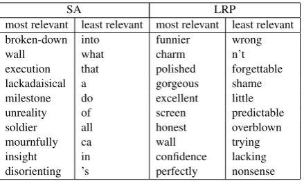
Table 1: Ten most resp. least relevant words iden-tified by SA and LRP over all 2210 test sentences, using as relevance target class the class “very pos-itive”.
word lists, we observe that the highest SA rele-vances mainly point to words with a strong se-mantic meaning, but not necessarily expressing a positive sentiment, see e.g. broken-down, lack-adaisicalandmournfully, while the lowest SA rel-evances correspond to stop words. On the con-trary, the extremal LRP relevances are more re-liable: the highest relevances indicate words ex-pressing a positive sentiment, while the lowest rel-evances are attributed to words defining a negative sentiment, hence both extremal relevances are re-lated in a meaningful way to the target class of interest, i.e. the class “very positive”.
4.3 Validation of Word Relevance
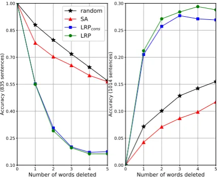
In order to quantitatively validate the word-level relevances obtained with SA and LRP, we perform two word deleting experiments. For these experi-ments we consider only test set sentences with a length greater or equal to 10 words (this amounts to retain 1849 test sentences), and we delete from each sentence up to 5 words accordingly to their SA resp. LRP relevance value (for deleting a word we simply set its word embedding to zero in the input sentence representation), and re-predict via the bi-LSTM the sentiment of the sentence with “missing” words, to track the impact of these dele-tions on the classifier’s decision. The idea behind this experiment is that the relevance decomposi-tion method that most pertinently reveals words that are important to the classifier’s decision, will impact the most this decision when deleting words accordingly to their relevance value. Prior to the deletions, we first compute the SA resp. LRP word-level relevances on the original sentences (with no word deleted), using the true sentence
sentiment as target class for the relevance decom-position. Then, we conduct two types of dele-tions. On initially correctly classified sentences we delete words in decreasing order of their rel-evance value, and on initially falsely classified sentences we delete words in increasing order of their relevance. We additionally perform a random word deletion as an uninformative variant for com-parison. Our results in terms of tracking the clas-sification accuracy over the number of word dele-tions per sentence are reported in Fig. 3. These results show that, in both considered cases, delet-ing words in decreasdelet-ing or increasdelet-ing order of their LRP relevance has the most pertinent effect, sug-gesting that this relevance decomposition method is the most appropriate for detecting words speak-ingfororagainsta classifier’s decision. While the LRP variant with relevance conservation LRPcons
performs almost as good as standard LRP, the lat-ter yields slightly superior results and thus should be preferred. Finally, when deleting words in increasing order of their relevance value starting with initially falsely classified sentences (Fig. 3
right), we observe that SA performs even worse than random deletion. This indicates that the low-est SA relevances point essentially to words that have no influence on the classifier’s decision at all, rather that signalizing words that are “inhibiting” it’s decision and speaking against the true class, as LRP is indeed able to identify. Similar conclu-sions were drawn when comparing SA and LRP on a convolutional network for document classifi-cation (Arras et al.,2016a).
4.4 Relevance Distribution over Sentence Length
0 1 2 3 4 5 Number of words deleted 0.10
0.25 0.40 0.55 0.70 0.85 1.00
Ac
cu
rac
y (
83
5 se
nte
nc
es)
random SA LRPcons LRP
0 1 2 3 4 5
Number of words deleted 0.00
0.05 0.10 0.15 0.20 0.25 0.30
Ac
cu
rac
y (
10
14
se
nte
nc
[image:7.595.74.288.63.237.2]es)
Figure 3: Impact of word deleting on initially cor-rectly (left) and falsely (right) classified test sen-tences, using either SA or LRP as relevance de-composition method (LRPconsis a variant of LRP
with relevance conservation). The relevance tar-get class is the true sentence class, and words are deleted in decreasing (left) and increasing (right) order of their relevance. Random deletion is aver-aged over 10 runs (std<0.016). A steep decline (left) and incline (right) indicate informative word relevance.
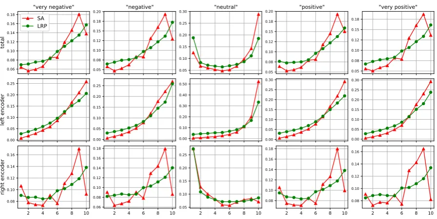
either the total word relevance obtained via the bi-LSTM model, or by considering only the part of the relevance that comes from one of the two unidirectional model constituents, i.e. the rele-vance contributed by the LSTM which takes as in-put the sentence words in their original order (we call it left encoder), or the one contributed by the LSTM which takes as input the sentence words in reversed order (we call it right encoder). The re-sulting distributions, for different relevance target classes, are reported in Fig. 4. Interestingly, the relevance distributions are not symmetric w.r.t. to the sentence middle, and the major part of the rel-evance is attributed to the second half of the sen-tences, except for the target class “neutral”, where the most relevance is attributed to the last com-putational time steps of the left or the right en-coder, resulting in an almost symmetric distribu-tion of the total relevance for that class. This can maybe be explained by the fact that, at least for longer movie reviews, strong judgments on the movie’s quality tend to appear at the end of the sentences, while the beginning of the sentences serves as an introduction to the review’s topic, de-scribing e.g. the movie’s subject or genre. Another
particularity of the relevance distribution we no-tice, is that the relevances of the left encoder tend to be more smooth than those of the right encoder, which is a surprising result, as one might expect that both unidirectional model constituents behave similarly, and that there is no mechanism in the model to make a distinction between the text read in original and in reversed order.
5 Conclusion
In this work we have introduced a simple yet effective strategy for extending the LRP proce-dure to recurrent architectures, such as LSTMs, by proposing a rule to backpropagate the rele-vance through multiplicative interactions. We ap-plied the extended LRP version to a bi-directional LSTM model for the sentiment prediction of sen-tences, demonstrating that the resulting word rel-evances trustworthy reveal words supporting the classifier’s decisionfororagainsta specific class, and perform better than those obtained by a gradient-based decomposition.
Our technique helps understanding and verify-ing the correct behavior of recurrent classifiers, and can detect important patterns in text datasets. Compared to other non-gradient based explana-tion methods, which rely e.g. on random sampling or on iterative representation occlusion, our tech-nique is deterministic, and can be computed in one pass through the network. Moreover, our method is self-contained, in that it does not require to train an external classifier to deliver the explanations, these are obtained directly via the original classi-fier.
Future work would include applying the pro-posed technique to other recurrent architectures such as character-level models or GRUs, as well as to extractive summarization. Besides, our method is not restricted to the NLP domain, and might also be useful to other applications relying on recurrent architectures.
Acknowledgments
0.06 0.08 0.10 0.12 0.14 0.16 0.18 to ta l "very negative" SA LRP 0.00 0.05 0.10 0.15 0.20 0.25 le ft e nc od er
2 4 6 8 10
0.08 0.10 0.12 0.14 0.16 ri gh t en co de r 0.05 0.08 0.10 0.12 0.15 0.18 0.20 "negative" 0.00 0.05 0.10 0.15 0.20 0.25
2 4 6 8 10
0.06 0.08 0.10 0.12 0.14 0.16 0.18 0.05 0.10 0.15 0.20 0.25 0.30 "neutral" 0.00 0.10 0.20 0.30 0.40 0.50
2 4 6 8 10
0.05 0.10 0.15 0.20 0.25 0.05 0.08 0.10 0.12 0.15 0.18 0.20 "positive" 0.00 0.05 0.10 0.15 0.20 0.25 0.30
2 4 6 8 10
0.08 0.10 0.12 0.14 0.16 0.18 0.05 0.08 0.10 0.12 0.15 0.18 "very positive" 0.00 0.05 0.10 0.15 0.20 0.25 0.30
2 4 6 8 10
[image:8.595.75.524.61.286.2]0.08 0.10 0.12 0.14 0.16
Figure 4: Word relevance distribution over the sentence length (divided into 10 intervals), per relevance target class (indicated on the top), obtained by performing SA and LRP on all test sentences having a length greater or equal to 19 words (1104 sentences). For LRP, the absolute value of the word-level relevances is used to compute these statistics. The first row corresponds to the total relevance, the second resp. third row only contain the relevance from the bi-LSTM’s left and right encoder.
References
Leila Arras, Franziska Horn, Gr´egoire Montavon, Klaus-Robert M¨uller, and Wojciech Samek. 2016a. Explaining Predictions of Non-Linear Classifiers in NLP. InProceedings of the ACL 2016 Workshop on Representation Learning for NLP. Association for Computational Linguistics, pages 1–7.
Leila Arras, Franziska Horn, Gr´egoire Montavon, Klaus-Robert M¨uller, and Wojciech Samek. 2016b. ”What is Relevant in a Text Document?”: An In-terpretable Machine Learning Approach. arXiv 1612.07843.
Sebastian Bach, Alexander Binder, Gr´egoire Mon-tavon, Frederick Klauschen, Klaus-Robert M¨uller, and Wojciech Samek. 2015. On Pixel-Wise Ex-planations for Non-Linear Classifier Decisions by Layer-Wise Relevance Propagation. PLOS ONE 10(7):e0130140.
Kyunghyun Cho, Bart van Merrienboer, Caglar Gul-cehre, Dzmitry Bahdanau, Fethi Bougares, Hol-ger Schwenk, and Yoshua Bengio. 2014. Learn-ing Phrase Representations usLearn-ing RNN Encoder-Decoder for Statistical Machine Translation. In Pro-ceedings of the 2014 Conference on Empirical Meth-ods in Natural Language Processing (EMNLP). Association for Computational Linguistics, pages 1724–1734.
Misha Denil, Alban Demiraj, and Nando de Freitas. 2014. Extraction of Salient Sentences from Labelled Documents. arXiv1412.6815.
Yannis Dimopoulos, Paul Bourret, and Sovan Lek. 1995. Use of some sensitivity criteria for choosing networks with good generalization ability. Neural Processing Letters2(6):1–4.
Felix A. Gers, J¨urgen Schmidhuber, and Fred Cum-mins. 2000. Learning to Forget: Continual Predic-tion with LSTM. Neural Computation12(10):2451– 2471.
Muriel Gevrey, Ioannis Dimopoulos, and Sovan Lek. 2003. Review and comparison of methods to study the contribution of variables in artificial neural net-work models. Ecological Modelling 160(3):249– 264.
Sepp Hochreiter and J¨urgen Schmidhuber. 1997. Long Short-Term Memory. Neural Computation 9(8):1735–1780.
Will Landecker, Michael D. Thomure, Lu´ıs M. A. Bet-tencourt, Melanie Mitchell, Garrett T. Kenyon, and Steven P. Brumby. 2013. Interpreting Individual Classifications of Hierarchical Networks. In IEEE Symposium on Computational Intelligence and Data Mining (CIDM). pages 32–38.
Sebastian Lapuschkin, Alexander Binder, Gr´egoire Montavon, Klaus-Robert M¨uller, and Wojciech Samek. 2016. The Layer-wise Relevance Propaga-tion Toolbox for Artificial Neural Networks. Jour-nal of Machine Learning Research17(114):1–5. Jiwei Li, Xinlei Chen, Eduard Hovy, and Dan
Models in NLP. In Proceedings of the 2016 Con-ference of the North American Chapter of the Asso-ciation for Computational Linguistics: Human Lan-guage Technologies (NAACL-HLT). pages 681–691. Jiwei Li, Will Monroe, and Dan Jurafsky. 2016b. Un-derstanding Neural Networks through Representa-tion Erasure. arXiv1612.08220.
Saif M. Mohammad. 2017. Challenges in Sentiment Analysis. In Erik Cambria, Dipankar Das, Sivaji Bandyopadhyay, and Antonio Feraco, editors, A Practical Guide to Sentiment Analysis. Springer In-ternational Publishing, pages 61–83.
Gr´egoire Montavon, Sebastian Lapuschkin, Alexander Binder, Wojciech Samek, and Klaus-Robert M¨uller. 2017a. Explaining nonlinear classification decisions with deep Taylor decomposition. Pattern Recogni-tion65:211–222.
Gr´egoire Montavon, Wojciech Samek, and Klaus-Robert M¨uller. 2017b. Methods for Interpreting and Understanding Deep Neural Networks. arXiv 1706.07979.
James Murdoch and Arthur Szlam. 2017. Automatic Rule Extraction from Long Short Term Memory Networks. InInternational Conference on Learning Representations Conference Track (ICLR).
Preslav Nakov, Alan Ritter, Sara Rosenthal, Fabrizio Sebastiani, and Veselin Stoyanov. 2016. SemEval-2016 Task 4: Sentiment Analysis in Twitter. In Pro-ceedings of the 10th International Workshop on Se-mantic Evaluation (SemEval-2016). Association for Computational Linguistics, pages 1–18.
Marco Tulio Ribeiro, Sameer Singh, and Carlos Guestrin. 2016. ”Why Should I Trust You?”: Ex-plaining the Predictions of Any Classifier. In Pro-ceedings of the 22nd ACM SIGKDD International Conference on Knowledge Discovery and Data Min-ing. pages 1135–1144.
David E. Rumelhart, Geoffrey E. Hinton, and Ronald J. Williams. 1986. Learning representations by back-propagating errors.Nature323:533–536.
Wojciech Samek, Alexander Binder, Gr´egoire Mon-tavon, Sebastian Lapuschkin, and Klaus-Robert M¨uller. 2017. Evaluating the visualization of what a Deep Neural Network has learned. IEEE Trans-actions on Neural Networks and Learning Systems PP(99):1–14.
Mike Schuster and Kuldip K. Paliwal. 1997. Bidirec-tional Recurrent Neural Networks. IEEE Transac-tions on Signal Processing45(11):2673–2681. Karen Simonyan, Andrea Vedaldi, and Andrew
Zis-serman. 2014. Deep Inside Convolutional Net-works: Visualising Image Classification Models and Saliency Maps. In International Conference on Learning Representations Workshop Track (ICLR).
Richard Socher, Alex Perelygin, Jean Y. Wu, Jason Chuang, Christopher D. Manning, Andrew Y. Ng, and Christopher Potts. 2013. Recursive Deep Mod-els for Semantic Compositionality Over a Sentiment Treebank. In Proceedings of the 2013 Conference on Empirical Methods in Natural Language Pro-cessing (EMNLP). Association for Computational Linguistics, pages 1631–1642.
Matthew D. Zeiler and Rob Fergus. 2014. Visualiz-ing and UnderstandVisualiz-ing Convolutional Networks. In Computer Vision ECCV 2014: 13th European Con-ference. pages 818–833.
Appendix
Long-Short Term Memory Network (LSTM)
We define in the following the LSTM recurrence equations (Hochreiter and Schmidhuber, 1997;
Gers et al.,2000) of the model we used in our ex-periments:
it=sigm
Wi ht−1+Ui xt+bi
ft=sigm
Wf ht−1+Uf xt+bf
ot=sigm
Woht−1+Uo xt+bo
gt=tanh
Wg ht−1+Ug xt+bg
ct=ftct−1 + itgt
ht=ottanh(ct)
Here above the activation functions sigm and
tanh are applied element-wise, and is an element-wise multiplication.
As an input, the LSTM gets fed with a sequence of vectors x = (x1, x2, ..., xT) representing the
word embeddings of the input sentence’s words. The matrices W’s, U’s, and vectors b’s are con-nection weights and biases, and the initial states
h0 andc0 are set to zero.
The last hidden state hT is eventually attached
to a fully-connected linear layer yielding a predic-tion score vector f(x), with one entryfc(x)per
class, which is used for sentiment prediction.
Bi-directional LSTM The bi-directional LSTM (Schuster and Paliwal,1997) we use in the present work, is a concatenation of two separate LSTM models as described above, each of them taking a different sequence of word embeddings as input.
One LSTM takes as input the words in their original order, as they appear in the input sentence. The second LSTM takes as input the same words but inreversedorder.
Each of these LSTMs yields a final hidden state vector, say h→