SemEval 2019 Task 12: Toponym Resolution in Scientific Papers

Proceedings of the 13th International Workshop on Semantic Evaluation (SemEval-2019), pages 907–916 907

SemEval-2019 Task 12: Toponym Resolution in Scientific Papers

Davy Weissenbacher†, Arjun Magge‡, Karen O’Connor†, Matthew Scotch‡, Graciela Gonzalez-Hernandez†

†_{DBEI, The Perelman School of Medicine, University of Pennsylvania,}

Philadelphia, PA 19104, USA

‡_{Biodesign Center for Environmental Health Engineering, Arizona State University,}

Tempe, AZ 85281, USA

†_{{dweissen, karoc, gragon}@pennmedicine.upenn.edu}

‡_{{amaggera, Matthew.Scotch}@asu.edu}

Abstract

We present the SemEval-2019 Task 12 which focuses on toponym resolution in scientific ar-ticles. Given an article from PubMed, the task consists of detecting mentions of names of places, or toponyms, and mapping the mentions to their corresponding entries in GeoNames.org, a database of geospatial loca-tions. We proposed three subtasks. In Sub-task 1, we asked participants to detect all ponyms in an article. In Subtask 2, given to-ponym mentions as input, we asked partici-pants to disambiguate them by linking them to entries in GeoNames. In Subtask 3, we asked participants to perform both the de-tection and the disambiguation steps for all toponyms. A total of 29 teams registered, and 8 teams submitted a system run. We summarize the corpus and the tools created for the challenge. They are freely available athttps://competitions.codalab. org/competitions/19948. We also an-alyze the methods, the results and the errors made by the competing systems with a focus on toponym disambiguation.

1 Introduction

Toponym resolution, also known as geoparsing, geo-grounding or place name resolution, aims to assign geographic coordinates to all location names mentioned in documents. Toponym res-olution is usually performed in two independent steps. First, toponym detection or geotagging, where the span of place names mentioned in a doc-ument is noted. Second, toponym disambiguation or geocoding, where each name found is mapped to latitude and longitude coordinates correspond-ing to the centroid of its physical location. To-ponym detection has been extensively studied in named entity recognition: location names were one of the first classes of named entities to be detected in text (Piskorski and Yangarber,2013).

Disambiguation of toponyms is a more recent task (Leidner,2007).

With the growth of the internet, the public adop-tion of smartphones equipped with Geographic In-formation Systems and the collaborative devel-opment of comprehensive maps and geographi-cal databases, toponym resolution has seen an im-portant gain of interest in the last two decades. Not only academic but also commercial and open source toponym resolvers are now available. How-ever, their performance varies greatly when ap-plied on corpora of different genres and domains (Gritta et al., 2018). Toponym disambiguation tackles ambiguities between different toponyms, like Manchester, NH, USA vs. Manchester, UK (Geo-Geo ambiguities), and between toponyms and other entities, such as names of people or daily life objects (Geo-NonGeo ambiguities). Ad-ditional linguistic challenges during the resolution step may be metonymic usage of toponyms, “91% of the US didn’t vote for either Hilary or Trump” (a country does not vote, thus the toponym refers to the people living in the country), elliptical con-structions, “Lakeview and Harrison streets” (the phrase refers to two street names Lakeview street and Harrison street), or when the context simply does not provide enough evidences for the resolu-tion.

Although significant progress has been made in the last decade on toponym resolution, it is still difficult to determine precisely the current state-of-the-art performances (Leidner and Lieberman,

Moreover, one corpus is not sufficient to evaluate a toponym resolver thoroughly, as the domain of a corpus strongly impacts the performance of a re-solver. A disambiguation strategy can be optimal on one domain and damaging on another. In ( Spe-riosu, 2013), Speriosu illustrates that toponyms occurring in historical literature will tend to re-solve within a local vicinity, whereas toponyms occurring in international press news refer to the most prominent places by default. Otherwise ad-ditional information is provided to help the reso-lution (ex. Paris, the city in Texas).

In this article we first define the concept of to-ponym and detail the subtasks of this challenge (Section 3). Then, we summarize how we ac-quired and annotated our data (Section4). In Sec-tion5, after describing the evaluation metrics, we briefly describe the resources and the baseline sys-tem provided to the participants. In the last Sec-tion6we discuss the results obtained and the po-tential future direction for the task of toponym res-olution.

2 Related Work

The Entity Linking task aims to map a name of an entity with the ID of the corresponding en-tity in a predefined Knowledge database (Bada,

2014). Entity linking has been largely studied by the community (Shen et al.,2015). Toponym res-olution is a special case of the entity linking task where strategies dedicated to toponyms can im-prove overall performances. Three main strate-gies have been proposed in the literature. The first exploits the linguistic context where a toponym is mentioned in a document. The vicinity of the toponym often contains clues that help the read-ers to interpret it. These clues can be other to-ponyms (Tobin et al.,2010), other named entities (Roberts et al.,2010), or even more generally, spe-cific topics associated more often with a particular toponym than with others (Speriosu,2013;Adams and McKenzie, 2013; Ju et al., 2016). The sec-ond strategy relies on the physical properties of the toponyms to disambiguate their mentions in documents. The population heuristic or the min-imum distance heuristic are popular heuristics us-ing such properties. The population heuristics dis-ambiguates toponyms by taking, among the am-biguous candidates, the candidate with the largest population, whereas the minimum distance heuris-tic disambiguates all toponyms in a document by

taking the set of candidates that are the closest to each other (Leidner, 2007). A recent heuris-tic computes from Wikipedia a network express-ing important toponyms and their semantic rela-tion with other entities. The network is then used to disambiguate jointly all toponyms in a doc-ument (Hoffart and Weikum, 2013; Spitz et al.,

2016). The last strategy is less frequently used as it depends on metadata describing the doc-uments where toponyms are mentioned. These metadata are of various kinds, but they all indi-cate, directly or not, geographic areas to help in-terpret toponyms mentioned in documents. Such metadata can be geotagging of social media posts (Zhang and Gelernter,2014) or external databases structuring the information detailed in a document (Weissenbacher et al., 2015). These three strate-gies are complementary and can be unified with machine learning algorithms as shown by (Santos et al.,2015) or (Kamalloo and Rafiei,2018).

3 Task Description

The definition of toponym is still in debate among researchers. In its simpler definition, a toponym is a proper name of an existing populated place on Earth. This definition can be extended to include a place or geographical entity that is named, and can be designated by a geographical coordinate1. This encompasses cities and countries, but also lakes or monuments. In this challenge we consider the extended definition of toponyms and exclude all indirect mentions of places such as “30 km north from Boston”, as well as metonymic usage and el-liptical constructions of toponyms.

Subtask 1: Toponym Detection Toponym de-tection consists of detecting the text boundaries of all toponym mentions in full PubMed articles. For example, given the sentence An H1N1 virus was isolated in 2009 from a child hospitalized in Nanjing, China., a perfect detector, regardless how, would return two pairs encoding the starting and ending positions of Nanjing and China,i.e. (64, 70) and (73, 77). Despite major progress, toponym detection is still an open problem and it was evaluated in a separate subtask since it determines the overall performance of the resolution. Toponym mentions missed during the detection cannot be disam-biguated (False Negative, FN) and, inversely,

1_{https://unstats.un.org/unsd/geoinfo/}

phrases wrongly detected as toponyms will re-ceived geocoordinates during the disambiguation (False Positive, FP). Both FNs and FPs degrade the quality of the overall resolution.

Subtask 2: Toponym Disambiguation The second subtask focuses on the disambiguation of the toponyms only. In this subtask, all names of locations in articles are known by a disambigua-tor but not their precise coordinates. The disam-biguator has to select the GeoNames IDs corre-sponding to the expected places among all pos-sible candidates. GeoNames2 is a crowdsourced database of geospatial locations and freely avail-able. Following with our previous example, given the position of Nanjing in the sentence, a per-fect disambiguator, regardless how, would have to choose among 12 populated places named Nanjing located in China in GeoNames and return the en-try 7843770 in GeoNames. The disambiguator has to infer the expected place based on all informa-tion available in the article and not only based on the sentence. This subtask allows one to measure the performance of the disambiguation algorithms independently from the performances of the to-ponym detector used upstream.

Subtask 3: End-to-end, Toponym Resolution

The last subtask evaluates the toponym resolver as it would be when deployed in real-world applica-tions. Only the full PubMed articles are given to the resolver and all toponyms detected and disam-biguated by the resolver are evaluated.

4 Data and Resources

4.1 A Case Study: Epidemiology of Viruses

The automatic resolution of the names of places mentioned in textual documents has multiple ap-plications and, therefore, has been the focus of re-search for both industrial and academic organiza-tions. For this challenge, we chose a scientific do-main where the resolution of the names of places is key: epidemiology.

One aim in epidemiology might be to create maps of the locations of viruses and their migra-tion paths, a tool which is used to monitor and intervene during disease epidemics. To create maps of viruses, researchers often use geospatial metadata of individual sequence records in public databases such as NIH’s GenBank (Benson et al.,

2_{https://www.geonames.org/}

2017)3. The metadata provides the location of the infected host. With more than 3 million virus se-quences4, GenBank provides abundant informa-tion on viruses. However, previous work has sug-gested that geospatial metadata, when it is not sim-ply missing, can be too imprecise for local-scale epidemiology (Scotch et al., 2011). In their ar-ticle Scotch et al., 2011 estimate that only 20% of GenBank records of zoonotic viruses contain detailed geospatial metadata such as a county or a town name (zoonotic viruses are viruses able to infect naturally hosts of different species, like rabies). Most GenBank records provide generic information, such as Japan or Australia, without mentioning the specific places within these coun-tries. However, more specific information about the locations of the viruses may be present in arti-cles which describe the research work. To create a complete map, researchers are then forced to read these articles to locate in the text these additional pieces of geospatial metadata for a set of viruses of interest. This manual process can be highly time-consuming and labor-intensive.

This challenge was an opportunity to assess the development and evaluation of automated ap-proaches to retrieve geospatial metadata with finer level of granularity from full-text journal arti-cles, approaches that can be further transferred or adapted to resolve names of places in other scien-tific domains.

4.2 Corpus Collection

Our corpus is composed of 150 full text journal articles downloaded from the subset of PubMed Central (PMC) in open access5. All articles in this subset of PMC are covered by a Creative Com-mons license and free to access. We built our cor-pus using three queries on GenBank.

Subset A: For the first 60 articles, we down-loaded 102,949 GenBank records that were linked to NCBI taxonomy id 197911 for influenza A. The downloaded records were associated with 1,424 distinct PubMed articles and 598 of them had links

3

For this competition we chose to work with PubMed ar-ticles and the GenBank database as they provide more com-plete and detailed information for epidemiology than public health reports.

4_{Last accessed April 2019 with the query:}

https://www.ncbi.nlm.nih.gov/nuccore/ ?term=txid10239[Organism:exp]

5_{https://www.ncbi.nlm.nih.gov/pmc/}

to an open access journal article in PubMed Cen-tral (PMC). We randomly sampled 60 articles from this set of 598 articles for manual annotation.

Subset B: We selected 60 additional articles by expanding our search to GenBank records linked to influenza B and C, rabies, hantavirus, west-ern equine encephalitis, eastwest-ern equine encephali-tis, St. Louis encephaliencephali-tis, and West Nile virus. Our query returned a total of 544,422 GenBank records. We randomly selected a subset of records associated with 1,915 unique open access PMC articles. From these 1,915 articles, we randomly selected for toponym annotation a stratified sam-ple of 60 articles, where strata were based on the number of GenBank records associated with the articles.

Subset C: We completed our corpus with 30 biomedical research articles to decrease bias and increase the generalizability of our corpus beyond toponym mentions in virus related research arti-cles. From the 1,341 research articles returned by the search in PMC of the journal titles with the Article Attribute of Open access, we randomly se-lected 30 articles from top epidemiology journals, as determined by their impact factor in September 2018.

Since the 60 articles from Subset A had been used in our prior publications (Weissenbacher et al.,2015,2017), we kept them all for training. We randomly selected half of the articles from Subset B and Subset C for training and left the sec-ond half for testing. The resulting corpus of 105 articles for training and 45 for testing was used for all three subtasks of the competition. The corpus is available for download on the Codalab used for the competition: https://competitions. codalab.org/competitions/20171# learn_the_details-data_resources.

4.3 Annotation Process

To perform the annotation, we manually down-loaded the PDF versions of the PMC articles and converted them to text files using the freely avail-able tool, Pdf-to-text6. We formatted the output to be compatible with the BRAT annotator7 ₍ Stene-torp et al., 2012). We manually detected and disambiguated the toponyms using GeoNames. We annotated toponyms in titles, bodies, tables

6

http://www.foolabs.com/xpdf/download

7_{http://brat.nlplab.org/index.html}

and captions sections of the documents. We re-moved contents that would not contain virology-related toponyms, such as the names of the au-thors, acknowledgments and references, this was done manually. In cases where a toponym could not be found in GeoNames, we set its coordinates to a special value N/A. Prior to beginning annota-tion, we developed a set of annotation guidelines after discussion among three annotators. The re-sulting guidelines are also available in the Codalab of the competition. Two annotators were under-graduate students in biomedical informatics and biology, respectively, and our senior annotator has a M.S. in biomedical informatics.

Two annotators annotated independently 58 ar-ticles of Subset B to estimate the inter-annotator agreement. Since the detection task is a named-entity recognition task, we followed the recom-mendations of Rothschild and Hripcsak (2005) and used precision and recall metrics to estimate the inter-annotator rate. The inter-annotator agree-ment rate on the toponym detection was .94 preci-sion (P) and .95 recall (R) which indicates a good agreement between the annotators. The inter-annotator agreement rate on the toponym disam-biguation was 0.857 Accuracy. Subset C was also annotated by two annotators, although not inde-pendently, to ensure the quality of the annotation of all documents occurring in the test set of the competition.

5 Evaluation

5.1 Toponym Resolution Metrics

When a gold standard corpus and a toponym resolver are aligned on the same geographical database, here the database GeoNames, the stan-dard metrics of precision, recall and F-measure can be used to measure the performance of the resolver. For this challenge, we report all results by using two common variations of these metrics: strict and overlapping measures. In the strict mea-sure, resolver annotations are considered matching with the gold standard annotations if they hit the same spans of text; whereas in overlapping mea-sure, both annotations match when they share a common span of text.

We computed the P and R for toponym detec-tion with the standard equadetec-tions: P recision =

T P/(T P+F P)andRecall=T P/(T P+F N), where TP (True Positive) is the number of to-ponyms correctly identified by a toponym detec-tor in the corpus, FP (False Positive) the number of phrases incorrectly identified as toponyms by the detector, and FN (False Negative) the number of toponyms not identified by the detector.

To evaluate the toponym disambiguation, we modified the equations computing the P and R used for toponym detection in order to account for both detection and disambiguation errors. The precision of the toponym disambiguation is given by the equation: P ds = T CD/T CD +T ID, where TCD is the number of toponyms correctly identified and disambiguated by the toponym dis-ambiguator in the corpus and TID is the number of toponyms incorrectly identified or incorrectly disambiguated in the corpus. The recall of the to-ponym disambiguation was computed by the equa-tion: Rds = T CD/T N, where TN is the total number of toponyms in the corpus. F1ds is the har-monic mean of Pds and Rds. Since the resolvers competing and the gold corpus annotations were aligned on GeoNames, toponyms correctly identi-fied were known by a simple match between the place IDs retrieved by the resolvers and those an-notated by the annotators.

5.2 Baseline System

We released an end-to-end system to be used as a strong baseline. This system performs sequen-tially the detection and the disambiguation of the toponyms in raw texts. To detect the toponyms the system uses a feedforward neural network

described in (Magge et al., 2018). The disam-biguation of all toponyms detected is then per-formed using a common heuristic, the population heuristic. Using this heuristic, the system always disambiguates a toponym by choosing the place which has the highest population in GeoNames. The baseline system can be downloaded from the Codalab website of the competition. We also made available to the participants a Rest service to search a recent copy of GeoNames, the documen-tation and the code to deploy the service locally can be found on the Codalab website.

6 Systems

6.1 Results

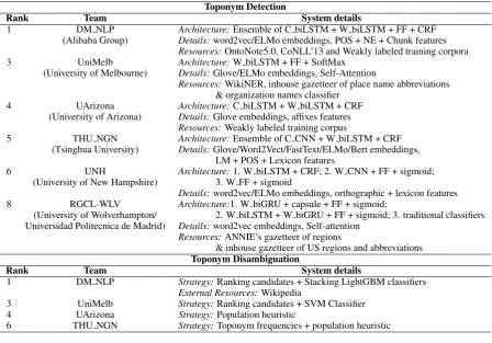
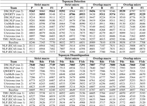
Twenty nine teams registered to participate in the shared-task and eight teams submitted. 21/8/13 submissions from 8/4/6 teams were included in the final evaluations of sub-task 1/2/3 respectively. All systems which attempted to resolve the toponyms in Subtask 3 opted for a pipeline architecture where the detection and the disambiguation steps were performed independently and sequentially. Table1summarizes the characteristics of the sys-tems along with their use of external resources. Tables 2, 3 and 4 presents the performances for each team. Team DM NLP achieved the best per-formances on all sub-tasks (Wang et al.,2019).

Toponym Detection

Rank Team System details

1 DM NLP Architecture:Ensemble of C biLSTM + W biLSTM + FF + CRF (Alibaba Group) Details:word2vec/ELMo embeddings, POS + NE + Chunk features

Resources:OntoNote5.0, CoNLL’13 and Weakly labeled training corpora 3 UniMelb Architecture:W biLSTM + FF + SoftMax

(University of Melbourne) Details:Glove/ELMo embeddings, Self-Attention

Resources:WikiNER, inhouse gazetteer of place name abbreviations & organization names classifier

4 UArizona Architecture:C biLSTM + W biLSTM + CRF (University of Arizona) Details:Glove embeddings, affixes features

Resources:Weakly labeled training corpus

5 THU NGN Architecture:Ensemble of C CNN + W biLSTM + CRF (Tsinghua University) Details:Glove/Word2Vect/FastText/ELMo/Bert embeddings,

LM + POS + Lexicon features

6 UNH Architecture:1. W biLSTM + CRF; 2. W CNN + FF + sigmoid;

(University of New Hampshire) 3. W FF + sigmoid

Details:word2vec/ELMo embeddings, orthographic + lexicon features 8 RGCL-WLV Architecture:1. W biGRU + capsule + FF + sigmoid;

(University of Wolverhampton/ 2. W biLSTM + W biGRU + FF + sigmoid; 3. traditional classifiers Universidad Politecnica de Madrid) Details:word2vec embeddings, Self-attention

Resources:ANNIE’s gazetteer of regions

& inhouse gazetteer of US regions and abbreviations

Toponym Disambiguation

Rank Team System details

1 DM NLP Strategy:Ranking candidates + Stacking LightGBM classifiers

External Resources:Wikipedia

3 UniMelb Strategy:Ranking candidates + SVM Classifier 4 UArizona Strategy:Population heuristic

6 THU NGN Strategy:Toponym frequencies + population heuristic

Table 1: System and resource descriptions for toponym resolution8_.

8

We use C biLSMT and C CNN to denote bidirectonal LSTMs or CNNs encoding sequences of characters, W biLSTM, W biGRU and W FF to denote bidirectional LSTMs/GRUs or Feed Forward encoders of word embeddings.

Strict macro Strict micro Overlap macro Overlap micro

Team P R F1 P R F1 P R F1 P R F1

DM NLP .9265 .9060 .9161 .9292 .8564 .8913 .9456 .9238 .9346 .9539 .8797 .9153

DM NLP .9214 .9010 .9111 .9222 .8512 .8853 .9447 .9224 .9334 .9510 .8776 .9128 DM NLP .9201 .9000 .9100 .9117 .8479 .8786 .9419 .9204 .9311 .9412 .8756 .9072 UniMelb .8827 .8598 .8711 .8469 .7748 .8092 .9222 .8911 .9064 .9135 .8283 .8688 QWERTY .9015 .8426 .8710 .8935 .7808 .8333 .9277 .8622 .8937 .9258 .8096 .8638 UArizona .8869 .8073 .8452 .8797 .7068 .7838 .9084 .8268 .8657 .9114 .7357 .8142 UArizona .8803 .8079 .8426 .8792 .7131 .7875 .9027 .8279 .8637 .9099 .7412 .8169 UArizona .8897 .7960 .8403 .8825 .6972 .7790 .9112 .8152 .8606 .9144 .7262 .8095 THU NGN .8897 .7818 .8323 .8647 .6615 .7496 .9221 .8125 .8639 .9136 .7025 .7943 THU NGN .8951 .7743 .8303 .8745 .6489 .7450 .9257 .8015 .8592 .9186 .6849 .7847 THU NGN .8966 .7699 .8284 .8715 .6497 .7444 .9254 .7961 .8559 .9197 .6892 .7879 UNH .8616 .7810 .8193 .8354 .6500 .7312 .9100 .8189 .8620 .8968 .7035 .7885 UniMelb .8402 .7967 .8179 .8023 .6768 .7342 .8866 .8398 .8626 .8795 .7440 .8061 UNH .8360 .7374 .7836 .8073 .6175 .6998 .9079 .7882 .8438 .9132 .6971 .7906 Baseline .8246 .7345 .7770 .8032 .5973 .6851 .8989 .7810 .8358 .9038 .6719 .7708 UNH .8111 .7403 .7741 .7819 .6459 .7074 .8859 .7984 .8399 .8904 .7372 .8066 NLP IECAS .8111 .6944 .7482 .7807 .5414 .6394 .8601 .7187 .7831 .8421 .5808 .6874 NLP IECAS .7527 .7226 .7373 .7298 .5796 .6461 .8209 .7700 .7946 .8155 .6457 .7207 NLP IECAS .7395 .7334 .7364 .7270 .5853 .6485 .8101 .7824 .7960 .8143 .6553 .7262 RGCL-WLV .8392 .4911 .6196 .8210 .3505 .4913 .9032 .5117 .6533 .8926 .3743 .5274 RGCL-WLV .8200 .4844 .6090 .8021 .3464 .4839 .8928 .5082 .6477 .8850 .3746 .5264 RGCL-WLV .8280 .4746 .6034 .8168 .3396 .4798 .8980 .4969 .6398 .8936 .3654 .5187

system which, according to their ablation study (Wang et al.,2019), proved to be effective9. Note that the performance of the first system is close to our IAA for toponym detection.

Toponym Disambiguation: All systems re-lied on handcrafted features to disambiguate to-ponyms. Their features described the lexical con-text of the toponyms and their importance. The importance of the toponyms was estimated by the frequencies of the candidates in the training data or by their populations. While the two top ranked systems combined such features with ma-chine learning, SVM for UniMelb and a gradient boosting algorithm for DM NLP, others just en-coded them into hard rules leading to suboptimal disambiguation.

6.2 Analysis

We analyzed a sample of errors to understand the remaining challenges for toponym disambiguation systems based on the results of Sub-task 2. We randomly selected 10 articles and analyzed 103 mentions of toponyms disambiguated incorrectly by all systems. We manually found 5 distinct cat-egories of errors. For the largest category of er-rors, with 62 cases, the systems missed context clues used by the authors of the articles to con-vey the correct interpretation of the toponym and chose the wrong candidates. Such clues include the mention of a country in the header of a table or the explicit mention of a district after an ambigu-ous toponym. 17 errors were due to the systems not complying with the guidelines, selecting in-stead populated places or cities when the expected choices were toponyms with a higher administra-tive level. 8 candidates were not found in GeoN-ames by strict or fuzzy matching because of their surface forms. These were unconventional abbre-viations, rare acronyms or words split by a hyphen. Despite our efforts to limit annotation errors, 15 were found in our sample10. The last error was a toponym where the choice made by the annotators can be argued.

9_{Team QWERTY did not describe their system at the time}

of writing. We were therefore unable to compare it with other systems.

10_{Since we analyzed entire articles, this count includes}

multiple mentions of the same toponym repeatedly annotated with the same error

7 Conclusion

In this paper we presented an overview of the re-sults of SemEval 2019 Task 12 which focuses on toponym resolution in scientific articles. Given an article from PubMed, the task consists of detect-ing all mentions of place names, or toponyms, in the article and mapping them to their correspond-ing entry in GeoNames, a database of geospatial locations. All systems resolved the toponyms in our corpus sequentially, detecting the toponyms before disambiguating them. Among the 21 sys-tems submitted for toponym detection, neural net-work based approaches were the most popular and the most efficient to detect toponyms with scores approaching the Inter-Annotator agreement. One key to success for the top ranked systems was to design two different algorithms to detect to-ponyms in the body and in the tables of the ar-ticles. The disambiguation of the toponyms re-mains challenging. Despite a clever use of rules or machine learning to combine features describing the lexical context of the toponyms and their im-portance from the 4 competing systems, the strict macro F1ds score of .82 of the best system sig-nals space for improvement. Our analysis of com-mon disambiguation errors reveals that it is still difficult for the systems to capture linguistic evi-dence in the context of the toponyms that dictate their disambiguation, causing 60% of the errors of the systems. The end-to-end performance of the best toponym resolver was .77 F1ds strict macro, a score high enough for scientists to benefit from au-tomation to reduce their workload when extracting toponyms from the voluminous and quickly grow-ing literature, while still leavgrow-ing room for techni-cal improvement.

Funding

Strict macro Strict micro

Team F1ds F1ds

DM NLP .8234 .7781

DM NLP .8215 .7821

UniMelb .8180 .7759

UniMelb .8180 .7759

DM NLP .8070 .7521

Baseline .7400 .6768 NLP IECAS .7233 .6582 NLP IECAS .7230 .6607

THU NGN .6721 .5886

Table 3: Results of the toponym disambiguation task, Subtask 2.

Toponym Detection

Strict macro Strict micro Overlap macro Overlap micro

Team P R F1 P R F1 P R F1 P R F1

DM NLP (run 2) .9265 .9060 .9161 .9292 .8564 .8913 .9456 .9238 .9346 .9539 .8797 .9153 QWERTY (run 1) .9203 .9095 .9148 .9214 .8706 .8953 .9438 .9311 .9374 .9501 .8972 .9229

DM NLP (run 1) .9214 .9010 .9111 .9222 .8512 .8853 .9447 .9224 .9334 .9510 .8776 .9128 DM NLP (run 3) .9201 .9000 .9100 .9117 .8479 .8786 .9419 .9204 .9311 .9412 .8756 .9072 UniMelb (run 2) .8821 .8598 .8708 .8464 .7748 .8090 .9215 .8911 .9061 .9130 .8283 .8686 UniMelb (run 1) .8884 .8124 .8487 .8767 .6986 .7776 .9349 .8442 .8872 .9322 .7448 .8280 UArizona (run 3) .8869 .8073 .8452 .8797 .7068 .7838 .9084 .8268 .8657 .9114 .7357 .8140 UArizona (run 2) .8803 .8079 .8426 .8792 .7131 .7875 .9027 .8279 .8637 .9099 .7412 .8169 UArizona (run 1) .8897 .7960 .8403 .8825 .6972 .7790 .9112 .8152 .8606 .9144 .7262 .8095 THU NGN (run 1) .8951 .7743 .8303 .8745 .6489 .7450 .9257 .8015 .8592 .9186 .6849 .7847 Baseline .8246 .7345 .7770 .8032 .5973 .6851 .8989 .7810 .8358 .9038 .6719 .7708 NLP IECAS (run 2) .8111 .6944 .7482 .7807 .5414 .6394 .8601 .7187 .7831 .8421 .5808 .6874 NLP IECAS (run 3) .8111 .6944 .7482 .7807 .5414 .6394 .8601 .7187 .7831 .8421 .5808 .6874 NLP IECAS (run 1) .7527 .7226 .7373 .7298 .5796 .6461 .8209 .7700 .7946 .8155 .6457 .7207

Toponym Disambiguation

Strict macro Strict micro Overlap macro Overlap micro

Team Pds Rds F1ds Pds Rds F1ds Pds Rds F1ds Pds Rds F1ds

DM NLP (run 2) .7840 .7661 .7749 .7601 .7005 .7291 .7887 .7715 .7800 .7646 .7060 .7341

DM NLP (run 1) .7762 .7587 .7674 .7513 .6934 .7212 .7840 .7667 .7753 .7593 .7019 .7295 QWERTY (run 1) .7597 .7506 .7551 .7336 .6931 .7128 .7677 .7586 .7631 .7417 .7016 .7211 UniMelb (run 2) .7437 .7276 .7355 .6848 .6268 .6545 .7510 .7368 .7438 .6964 .6399 .6670 UniMelb (run 1) .7286 .6711 .6987 .6876 .5479 .6098 .7331 .6777 .7043 .6941 .5564 .6177 UArizona (run 3) .6773 .6225 .6487 .6514 .5233 .5804 .6761 .6242 .6491 .6507 .5253 .5813 UArizona (run 2) .6739 .6243 .6482 .6533 .5299 .5852 .6725 .6256 .6482 .6521 .5313 .5855 UArizona (run 1) .6823 .6149 .6468 .6600 .5214 .5826 .6807 .6164 .6470 .6586 .5231 .5831 Baseline .6605 .5912 .6240 .6252 .4649 .5333 .6787 .6071 .6409 .6505 .4857 .5561 THU NGN (run 1) .6581 .5738 .6131 .6052 .4491 .5156 .6605 .5784 .6167 .6070 .4537 .5193 NLP IECAS (run 2) .6527 .5584 .6019 .6339 .4395 .5191 .6631 .5666 .6111 .6504 .4510 .5326 NLP IECAS (run 3) .6529 .5582 .6018 .6378 .4423 .5223 .6633 .5664 .6110 .6543 .4537 .5359 NLP IECAS (run 1) .5852 .5626 .5737 .5634 .4474 .4988 .5935 .5717 .5824 .5772 .4603 .5120 DM NLP (run 3) .0279 .0278 .0279 .0305 .0284 .0294 .0314 .0312 .0313 .0354 .0330 .0342

References

Benjamin Adams and Grant McKenzie. 2013. In-ferring Thematic Places from Spatially Referenced Natural Language Descriptions. Springer Nether-lands.

Michael Bada. 2014. Mapping of biomedical text to concepts of lexicons, terminologies, and ontologies.

Methods in Molecular Biology: Biomedical Litera-ture Mining, 1159:33–45.

Dennis A. Benson, Mark Cavanaugh, Karen Clark, Ilene Karsch-Mizrachi, David J. Lipman, James Os-tell, and Eric W. Sayers. 2017. Genbank. Nucleic Acids Research, 45(D):37–42.

Milan Gritta, Mohammad T. Pilehvar, Nut Lim-sopatham, and Nigel Collier. 2018. What’s missing in geographical parsing? Language Resources and Evaluation, 52(2):603–623.

Johannes Hoffart and Gerhard Weikum. 2013. Dis-covering and disambiguating named entities in text. In Proceedings of the 2013 SIGMOD/PODS Ph.D. Symposium, SIGMOD’13 PhD Symposium, pages 43–48. ACM.

Yiting Ju, Benjamin Adams, Krzysztof Janowicz, Yingjie Hu, Bo Yan, and Grant Mckenzie. 2016. Things and strings: Improving place name disam-biguation from short texts by combining entity co-occurrence with topic modeling. In 20th Interna-tional Conference on Knowledge Engineering and Knowledge Management - Volume 10024, EKAW 2016, pages 353–367. Springer-Verlag New York, Inc.

Ehsan Kamalloo and Davood Rafiei. 2018. A coherent unsupervised model for toponym resolution. In Pro-ceedings of the 2018 World Wide Web Conference, WWW ’18, pages 1287–1296. International World Wide Web Conferences Steering Committee.

Morteza Karimzadeh and Alan M. MacEachren. 2019. Geoannotator: A collaborative semi-automatic plat-form for constructing geo-annotated text corpora.

ISPRS International Journal of Geo-Information, 8(4).

Jochen L. Leidner. 2007. Toponym Resolution in Text: Annotation, Evaluation and Applications of Spatial Grounding of Place Names. Ph.D. thesis, Insti-tute for Communicating and Collaborative Systems School of Informatics, University of Edinburgh.

Jochen L. Leidner and Michael D. Lieberman. 2011. Detecting geographical references in the form of place names and associated spatial natural language.

SIGSPATIAL, 3(2):5–11.

Arjun Magge, Davy Weissenbacher, Abeed Sarker, Matthew Scotch, and Graciela Gonzalez-Hernandez. 2018. Deep neural networks and distant supervision for geographic location mention extraction. Bioin-formatics, 34(13):i565–i573.

Jakub Piskorski and Roman Yangarber. 2013. Informa-tion extracInforma-tion: Past, present and future. In Thierry Poibeau, Horacio Saggion, Jakub Piskorski, and Ro-man Yangarber, editors, Multi-source, Multilingual Information Extraction and Summarization, Theory and Applications of Natural Language Processing, pages 23–49. Springer Berlin Heidelberg.

Kirk E. Roberts, Cosmin A. Bejan, and Sanda M. Harabagiu. 2010. Toponym disambiguation using events. InFLAIRS Conference.

Adam S. Rothschild and George Hripcsak. 2005. Agreement, the f-measure, and reliability in infor-mation retrieval. Journal of the American Medical Informatics Association, 12(3):296–298.

Jo˜ao Santos, Ivo Anast´acio, and Bruno Martins. 2015. Using machine learning methods for disambiguating place references in textual documents. GeoJournal, 80(3):375–392.

Matthew Scotch, Indra N. Sarkar, Changjiang Mei, Robert Leaman, Kei-Hoi Cheung, Pierina Ortiz, Ashutosh Singraur, and Graciela Gonzalez. 2011. Enhancing phylogeography by improving geograph-ical information from genbank. Journal of Biomed-ical Informatics, 44(44-47).

Wei Shen, Jianyong Wang, and Jiawei Han. 2015. En-tity linking with a knowledge base: Issues, tech-niques, and solutions. IEEE Transaction on Knowl-edge and Data Engineering, 27(2).

Michael A. Speriosu. 2013.Methods and Applications of Text-Driven Toponym Resolution with Indirect Su-pervision. Ph.D. thesis, University of Texas.

Andreas Spitz, Johanna Geiß, and Michael Gertz. 2016. So far away and yet so close: Augmenting toponym disambiguation and similarity with text-based net-works. In Proceedings of the Third International ACM SIGMOD Workshop on Managing and Min-ing Enriched Geo-Spatial Data, GeoRich ’16, pages 2:1–2:6. ACM.

Pontus Stenetorp, Sampo Pyysalo, Goran Topi´c, Tomoko Ohta, Sophia Ananiadou, and Jun’ichi Tsu-jii. 2012. Brat: A web-based tool for nlp-assisted text annotation. InProceedings of the Demonstra-tions at the 13th Conference of the European Chap-ter of the Association for Computational Linguistics, EACL’12, pages 102–107. Association for Compu-tational Linguistics.

Richard Tobin, Claire Grover, Kate Byrne, James Reid, and Jo Walsh. 2010. Evaluation of georeferencing. InProceedings of the 6th Workshop on Geographic Information Retrieval, GIR ’10, pages 7:1–7:8.

Davy Weissenbacher, Abeed Sarker, Tasnia Tahsin, Matthew Scotch, and Graciela Gonzalez. 2017. Ex-tracting geographic locations from the literature for virus phylogeography using supervised and distant supervision methods. In In Proceedings of AMIA Joint Summits on Translational Science.

Davy Weissenbacher, Tasnia Tahsin, Rachel Beard, Mari Figaro, Robert Rivera, Matthew Scotch, and Graciela Gonzalez. 2015. Knowledge-driven geospatial location resolution for phylogeographic models of virus migration. Bioinformatics, 31(12):i348–i356.

Wei Zhang and Judith Gelernter. 2014. Geocoding lo-cation expressions in twitter messages: A preference learning method. J. Spatial Information Science, 9:37–70.

Abbreviations

POS: Part-Of-Speech

NER: Named Entity Recognition

LM: Language Model

ANNIE: A Nearly-New Information Extraction

SVM: Support Vector Machine

CRF: Conditional Random Field

FF: Feedforward

CNN: Convolutional Neural Network

biLSTM: bidirectional Long Short-Term Memory