Munich Personal RePEc Archive
A Note on Consistent Conditional
Moment Tests
Wang, Xuexin
he Wang Yanan Institute for Studies in Economics(WISE), Xiamen
University, Xiamen, Fujian, China
1 July 2015
Online at
https://mpra.ub.uni-muenchen.de/69005/
A NOTE ON CONSISTENT CONDITIONAL MOMENT
TESTS
Xuexin WANG∗
This Version: July 2015
Abstract
In this paper we propose a new consistent conditional moment test, which synergizes Bierens’ approach with the consistent test of overidentifying restrictions. It relies on a transformation-based empirical process combining both approaches. This new empirical pro-cess enjoys some advantages. Firstly it is not affected by the uncertainty from the parameter estimation. Moreover this estimation-effect-free property requires much less restrictive rate condition than in the consistent test of overidentifying restrictions alone. Furthermore the integrated conditional moment (ICM) test based on the new empirical process have power against Pitman local alternatives. We prove, under some regularity conditions, the admis-sibility of the ICM test based on this transformation-based empirical process in the case that there exists heteroskedasticity of unknown form, extending the result in Bierens and Ploberger (1997). The new consistent test also allows us to propose a much simpler boot-strap procedure than the standard ones. A version of Bierens (1990) test based on the new empirical process is also discussed, and its asymptotic properties are analyzed. Monte Carlo simulations show that Bierens (1990) test based on the new empirical process is more power-ful for a large number of alternatives when heteroskedasticity of unknown form is presented.
JEL Classification: C12 C21
Keywords: Consistent Conditional Moment Test; Consistent Test of Overidentifying
Re-strictions ; ICM Test; Admissibility
∗Address: The Wang Yanan Institute for Studies in Economics(WISE), Xiamen University, Xiamen, Fujian,
1
Introduction
Models based on conditional moment restrictions are quite prevalent in econometrics, arising in
many econometric settings. For example the rational expectations and dynamic asset pricing
models in macroeconomics and finance give rise to conditional moment restrictions in the form
of stochastic Euler equations. Other cases include panel data models and instrumental variable
regressions. In order to conduct convincing estimation and inference of these models, it is crucial
to check the validity of these conditional moment restrictions.
There is a vast amount of literature on consistently testing the correct specification of
con-ditional moment restrictions. Generally, these tests can be grouped into two classes. The first
class is based on smoothing methods, comparing the fitted parametric regression function with
a nonparametric function estimator, see, H¨ardle and Mammen (1993), Gozalo (1993), Hong and
White (1995), Fan and Li (1996), and Zheng (1996), to mention but a few. The
smoothing-based tests only require some consistent parameter estimator, and typically lead to asymptotic
pivotal test statistics under the null. However, they depend on a smoothing parameter, have no
power in Pitman local alternative generally, and there has been much concern over their small
sample properties. The second class of tests avoid smoothing estimation by means of converting
the conditional moment restriction into an infinite number of unconditional moment
restric-tions, see, for example, Bierens (1982, 1990), de Jong and Bierens (1994), Bierens and Ploberger
(1997), Stute (1997), Donald, Imbens and Newey (2003) and Escanciano (2006a). One strand
of literature in this class, which we would like to label as Bierens’ approach, considers a
contin-uum of unconditional moment restrictions implied by the conditional moment restrictions. It
relies on functionals of an empirical process, has to handle the uncertainty from the parameters
estimation, and leads to case-dependent limiting distributions. But it has power against Pitman
local alternatives. On the other hand, de Jong and Bierens (1994) and Donald et al. (2003)
propose consistent tests of overidentifying restrictions with the discrete number of unconditional
moment restrictions increasing with the sample size. Under some regularity conditions, the
nor-malized consistent tests of overidentifying restrictions are not affected by the estimation effects.
However they have no power against Pitman local alternatives, and they depend on a nuisance
parameter similar to the smoothing parameter in smoothing methods. Finally, Carrasco and
Florens (2000) and Dominguez and Lobato (2015) propose consistent tests of overidentifying
synergy of consistent tests of Bierens and the consistent tests of overidentifying restrictions.
In this paper we propose a new consistent conditional moment test, which synergizes Bierens’
approach with the consistent test of overidentifying restrictions. It relies on a
transformation-based empirical process combining both approaches. This new empirical process enjoys some
advantages. Firstly it is not affected by the uncertainty from the parameter estimation.
More-over this estimation-effect-free property requires much less restrictive rate condition than in
the consistent test of overidentifying restrictions alone. Furthermore the integrated conditional
moment (ICM) test based on the new empirical process have power against Pitman local
alter-natives. We prove, under some regularity conditions, the admissibility of the ICM test based
on this transformation-based empirical process in the case that there exists heteroskedasticity
of unknown form, extending the result in Bierens and Ploberger (1997). The new consistent
test also allows us to propose a much simpler bootstrap procedure than the standard ones.
A version of Bierens (1990) test based on the new empirical process is also discussed, and its
asymptotic properties are analyzed. Monte Carlo simulations show that Bierens (1990) test
based on the new empirical process is more powerful for a large number of alternatives when
heteroskedasticity of unknown form is presented.
The outline of the paper is as follows. In Section 2, we establish the preliminaries. In Section
3, we define the class of weighting functions, the new residual empirical process and study its
properties. Section 4 discusses the asymptotic theory of the ICM test. Section 5 establishes the
asymptotic admissibility of the ICM test when there exists heteroskedasticity of unknown form.
Section 6 propose a simple bootstrap for the ICM test. Section 7 discusses Bierens (1990)’s test
based on the new empirical process. Section 8 conducts Monte Carlo simulations. Section 9
concludes.
2
Preliminaries
let Z denote a single observation,θa p×1 vector of parameters, andX is ad×1 subvector of
Z. For a unique valueθ0∈Θ∈Rp, the following conditional moment restrictions hold
E[ρ(Z, θ0)|X] = 0 a.s. (1)
where ρ(Z, θ0) is a J ×1 vector of functions. It often can be thought of as residuals. In this
Example 1. Let Z = (Y, X′)′ be a random vector in a (1 +d)-dimensional Euclidean space, where X is a d×1 vector andY is a scalar. WhenE(|Y|)<∞, there exists a Borel measurable functionf such thatE(Y|X) =f(X). In parametric modeling,f(X) is assumed to belong to a parametric family G=f(X, θ) :Rd→R|θ∈Θ⊂Rp . In this case ρ(Z, θ
0) =Y −f(X, θ0).
In order to test whether model (1) is correctly specified, we need to test the following null
hypothesis
H0 :E[ρ(Z, θ0)|X] = 0 a.s., for θ0∈Θ, (2)
and the alternative hypothesis is
H1 :P(E[ρ(Z, θ)|X] = 0)<1 a.s., for allθ∈Θ. (3)
The idea of Bierens’ approach is to convert the conditional moment restriction into an infinite
number of unconditional moment restrictions, i.e,
E[ρ(Z, θ0)|X] = 0 a.s⇔E[ρ(Z, θ0)w(X, t)] = 0, for almost all t∈ T, (4)
where T ⊂ Rh, h ∈ N, and w(X, t) is a proper weighting function such that the equivalence (4) holds. There are many weighting functions meeting the requirement of (4). One example is
w(X, t) = exp (it′X) where i= √−1, T = Rd, which is employed by Bierens (1982). Bierens
(1990) proposes w(X, t) = exp (t′X), T = Rd. Stute (1997) proposes the indicator function
w(X, t) =I(X < t),T =Rd. Escanciano (2006a) introduces the weighting function w(X, t) =
I(β′X ≤u),with t= (β′, u)′ ∈ T =Sd×(−∞,∞), where Sd=β∈Rd:|β|= 1 .
Given a sampleZj,j= 1,· · ·, n, and a √n-consistent estimator ˆθ, the scaled sample analog
of E[ρ(Z, θ0)w(X, t)], which forms a residual empirical process, is
ˆ
Mθ, tˆ =n−1/2
n
X
j=1
ρ(Zj,θˆ)w(Xj, t) ,t∈Π⊂ T.
Stinchcombe and White (1998) coin this class of specification tests as the one with a nuisance
has the form
\
ICM = Z
Π
Mˆ θ, tˆ 2dµ(t),
whereµ(t) is a probability measure on Π that is absolutely continuous with respect to Lebesgue measure on Π⊂ T. Or we can maximize ˆMθ, tˆ over Π, resulting in a Kolmogorov-Smirnov type statistic
d
KS= sup
t∈Π
Mˆ θ, tˆ 2.
In contrast with smoothing-based tests, the bierens’ approach has to handle the uncertainty
from the parameter estimation. More specifically, it could be shown, under some regularity
conditions, that
ˆ
Mθ, tˆ =n−1/2
n
X
j=1
ρ(Zj, θ0)w(Xj, t) + ˆb(θ0, t)n1/2
ˆ
θ−θ0
+op(1),
where
ˆb(θ, t) = 1
n
n
X
j=1
w(Xj, t)
∂ρ(Zj, θ)
∂θ′ .
In most cases, ˆb(θ0, t)6= 0. The existence of the so-called “estimation effect” ˆb(θ0, t)n1/2
ˆ
θ−θ0
makes the asymptotic theory more complicated, and limit results dependent on the parameter
estimator employed.
While Bierens’ approach exploits a continuum of the unconditional moment restrictions, de
Jong and Bierens (1994) and Donald et al. (2003) show that it is sufficient to employ a set of
discrete countable unconditional moment restrictions in efficient estimation of parameters and
consistent test in the conditional moment restrictions models.1 More specifically, let U be the
support of distribution of X, define L2 be the space of measurable functions ϕ: U → R with
E[ϕ2(X)]<∞. We say a sequence of{qj(X)}∞j=1 inL2 isL2-complete if for any ε >0, and any
ϕ∈L2, there exists a positive integer K and a K×1 vectorγK such that
n
Ehϕ(X)−qK(X)′γK 2
io1/2
< ε, (5)
where qK(X) = (q1(X),· · · , qK(X))′ is a K×1 vector. Chamberlain (1987, 1992) show that
1
the asymptotic variance of the GMM estimator based on the unconditional moment restrictions
EqK(X)ρ(Z, θ0)= 0, whereqK(X) satisfies (5), comes arbitrarily close to the semiparametric
efficiency bound as K → ∞. Intuitively, since the conditional moment restriction is equivalent to a sequence of unconditional moment restrictions, as K grows with the sample size, all of the information of the conditional moment restriction is eventually accounted for. The GMM
estimator is obtained by minimizing the following objective function
ˆ
θGM M = arg min
θ∈Θ
n
X
j=1
qK(Xj)ρ(Zj, θ)
′
ˆ
Ω ¯θ, K−1
n
X
j=1
qK(Xj)ρ(Zj, θ)
,
where
ˆ
Ω (θ, K) = 1
n
n
X
i=1
ρ(Zi, θ)2qK(Xi)qK(Xi)′,
and ¯θ is some preliminary estimator of θ0. Hahn (1997) and Donald et al. (2003) establish
the rate condition of K for different choices of qK(X), for example splines and power series, in
efficient estimation ofθ0, reaching semiparametric efficient bound.
When it comes to consistent tests, the test statistic is in the form
ˆ
Tθ =n−1
n
X
j=1
qK(Xj)ρ(Zj, θ)
′
ˆ
Ω (θ, K)−1
n
X
j=1
qK(Xj)ρ(Zj, θ)
.
For a fixed K, ˆTθˆGM M is known to be chi-squared distribution with K −p degrees of freedom
asymptotically under the null hypothesis that the conditional moment restrictions are satisfied.
AsK grows with the sample size this approximation continues to hold. Normally the asymptotic normal approximation to the chi-square for large degrees of freedom is used. In this case, under
some rate condition ofK, a consistent estimator ˆθ, it has been shown that ˆ
Tθˆ−(K−p)
p
2 (K−p)
d
→N(0,1).
It should be noticed that the rate condition of K for consistent test is slower that the one for efficient estimation, see Donald et al. (2003). Furthermore it has no power against Pitman local
3
A Class of Weighting Functions and A New Empirical Process
In this section, we will synergize the Bierens’ approach with the consistent test of overidentifying
restrictions in a class of weighting functions. We focus on a class of weighting functions W such that
W =nw t′X, t∈Rd, wis an analytic function that is nonpolynomialo. For any weighting function in this class, we have the following lemma.
Lemma 1. Let X be a random vector in Rd, Φ(·) a bounded one-to-one mapping from Rd into
Rd, for any weighting function w(t′Φ(X)) in W, the equivalence in (4) holds.
Proof. See Stinchcombe and White (1998) Theorem 2.3.
Remark: Bierens and Ploberger (1997) give an alternative version of conditions of the
equiv-alence.
Examples of families satisfying this lemma arew(t′Φ(X)) = exp (it′Φ(X)) andw(t′Φ(X)) = exp (t′Φ(X)).
Forw∈ W and any t∈Π⊂Rd, we have a residual empirical process such that
ˆ
Mθ, tˆ =n−1/2
n
X
j=1
ρ(Zj,θˆ)w t′Φ(Xj)
.
On the other hand,w(t′Φ(X)) also forms a basis for the efficient parameters estimation and consistent test of overidentifying restrictions. For any fixed sequence {tj}∞j=1, which is dense in
some subset ofRd,q
j(X) =w(t′jΦ(X)), j= 1,2,· · ·, and for each positive integerK, define the
K×1 vector
qK(X) = w t′1Φ (X),· · ·w t′KΦ (X)′. (6) Note that we omit in the notation qK(X) the dependence on {t
j}Kj=1 sequence. We have the
following corollary:
Corollary 1. For any ε > 0, ϕ ∈L2, and for each K×1 vector qK(X) defined in (6), there
exist K×1 vectors γK such that (5) holds.
Proof. See Appendix.
Assumption 1. The data are i.i.d. The parameter space Θ is a compact subset of Rp. θ
0 ∈
int(Θ).
Assumption 2. √n(ˆθ−θ0) =Op(1).
Assumption 3. Esupθ∈Θρ(Z, θ)2|X<∞, σ2(θ, X) =Eρ(Z, θ)2|X is bounded away from
zero. There is δ(X) and α >0 such that for all θ,¯ θ∈Θ, ρ(Z,θ¯)−ρ(Z, θ)≤δ(X)θ¯−θα and Eδ(X)2<∞.
Assumption 4. ρ(Z, θ)is twice continuously differentiable in a open and convex neighborhood∆
ofθ0. Eh
∂
2
ρ(Z,θ)
∂θ∂θ′
iis bounded,Eh∂ρ(∂θZ,θ)∂ρ∂θ(Z,θ′ ) i
is nonsingular. E
supθ∈∆∂ρ∂θ(Z,θ)2
<∞, Ehsupθ∈∆|ρ(Z, θ)|4|Xi < ∞, and for all θ ∈ ∆, |ρ(Z, θ)−ρ(Z, θ0)| ≤ δ(X)||θ−θ0|| and
Eδ(X)2<∞. Ehsupt∈T |w(t′Φ (X))|4i<∞. K ≥p, EhqK(X)∂ρ∂θ(Z,θ′ ) i
is of full rank.
Assumption 5. Denote U as the support ofX, for eachK there is a constant scalarξ(K) and
matrix B such that q˜K(X) = BqK(X) for every X ∈ U, supX∈U
q˜K(X) ≤ ξ(K), √K ≤ ξ(K), and E q˜K(X) ˜qK(X)′ has smallest eigenvalue bounded away from zero.
Assumptions 1 is a standard regularity condition. It restricts our analysis to an i.i.d context.
It is possible to extend it to dependent data following De Jong (1996). Assumption 2 shows
that we only need a √n-consistent estimator. Since we are dealing with a testing problem, we do not present the identification conditions of parameter estimation explicitly. To obtain a
√
n-consistent estimator, only an identification condition as weak as Dominguez and Lobato’s (2004) is needed. Assumption 3 imposes some restrictions on second moment condition ofρ(Z, θ) and the smoothness of the functionρ(Z, θ). Assumption 4 is essential for asymptotic normality when the number of moment conditions is growing with the sample size. Assumption 5 imposes
a normalization on the approximate function, bounds the second moment restriction away from
singularity and restricts the magnitude of the series terms. The magnitude of the series terms
is important, playing a crucial role in the asymptotic theory of GMM estimation and test when
K increases with sample size n. Primitive conditions for this assumption are given in the case of w(·) = exp(·) when we discuss the improved Bierens (1990) statistic in Section 6.
In stead of focusing on the residual empirical process ˆMθ, tˆ on some interval Π, we propose a new empirical process, combiningw(t′Φ(Xj)) andqK(X). The idea is to form a new
weighting functions by a proper linear combination of w(t′Φ(X)) and qK(X) such that there does not exist the estimation effect for the transformed empirical process. More specifically,
˜
M(θ, t, K) =n−1/2
n
X
j=1
ρ(Zj, θ)
w(t
′Φ(Xj))−
ˆb(θ, t) ˆA(θ, K) ˆΛ (θ, K)′Ω (ˆ θ, K)−1qK(X
j)
, (7)
where the new weighting function depends on
ˆ
Λ (θ, K) = 1
n
n
X
i=1
qK(Xi)∂ρ(Zi, θ)
∂θ′ , ˆ
A(θ, K) =hΛ (ˆ θ, K)′Ω (ˆ θ, K)−1Λ (ˆ θ, K)i−1.
Remark: We will show in Theorem 1 that ˜M(θ, t, K) does not suffer from the estimation effect. The intuition behind the removal of the estimation effect is that the transformed weighting
functionw(t′Φ(X))−ˆb(θ, t) ˆA(θ, K) ˆΛ (θ, K)′Ω (ˆ θ, K)−1qK(X
j) is orthogonal to ∂ρ(∂θZj′,θ) now. Remark: The new empirical process combines Bierens’ approach and the consistent tests of
overidentifying restrictions. To see this point, we rewrite (7) into
˜
M(θ, t, K) = n−1/2
n
X
j=1
ρ(Zj, θ)w(t′Φ(Xj))
−ˆb(θ, t) ˆA(θ, K) ˆΛ (θ, K)′Ω (ˆ θ, K)−1n−1/2
n
X
j=1
qK(Xj)ρ(Zj, θ).
n−1/2Pnj=1ρ(Zj, θ)w(t′Φ(Xj)),t∈Π⊂ T is the element of Bierens’ approach,n−1/2Pnj=1qK(Xj)ρ(Zj, θ)
is the essential part of consistent tests of overidentifying restrictions.
Remark: The form of ˜M(θ, t, K) also has a connection with the martingale transformation approach employed by Stute et al. (1998). In their case, w(X, t) =I(X < t), but this function does not fall into the class W. While martingale transformation approach focuses on obtaining asymptotic distribution-free statistics, our transformation focuses on obtaining optimal statistics
under conditional moment restrictions.
In the following theorem, we will show the estimation-effect free property of the new empirical
process for any fixed K≥p.
Theorem 1. When Assumptions 1 to 4 hold,K is fixed andK ≥p, under H0, for anyt∈Π⊂
Rd, given a √nconsistent test θ, under the nullˆ
˜
and
˜
M(ˆθ, t, K)→d N0, s2(θ0, t, K), (9)
where
s2(θ0, t, K) =E
ρ(Z, θ0)2
h
w(t′Φ(X))−b(θ0, t)A(θ0, K)Λ (θ, K)′Ω (θ, K)−1qK(X)
i2
,
b(θ0, t) =E
w(X, t)∂ρ(Z, θ0)
∂θ′
,
Ω (θ0, K) =E ρ(Z, θ0)2qK(X)qK(X),
Λ (θ0, K) =E
qK(X)∂ρ(Z, θ0)
∂θ′
,
A(θ0, K) =
h
Λ (θ0, K)′Ω (θ0, K)−1Λ (θ0, K)
i−1
. Proof. See Appendix
Equation (8) shows that, unlike ˆMθ, tˆ , ˜M(ˆθ, t, K) does not suffer from the estimation effect for a fixed K-the empirical process evaluated at any √n-consistent estimator is asymp-totically the same as the empirical process evaluated at the true parameters. Note that, to
reach the estimation-effect-free property in consistent tests of overidentifying restrictions, it is
required that K should follow the rate condition K → ∞and ξ(K)2K2/n→ 0, see Donald et
al. (2003).
In order to obtain more powerful test we would like to allowK to increase with sample size
n. We observe ˆA(θ, K) is an estimate of the asymptotic variance matrix of the optimal GMM estimator, which will generally be bounded below by the semiparametric efficiency bound. So
We establish the asymptotic boundary of the new empirical process when K increases with sample size nin the following lemma. DenoteD(θ, X) =E∂ρ(∂θZ,θ)|X,
Lemma 2. When Assumptions 1 to 5 hold, under H0, for any t∈Π⊂Rd, whenK → ∞ and
ξ(K)2K/n→0,
ˆ
A(θ0, K)→p A∗(θ0)
where A∗(θ0) =ED(θ0, X)σ−2(θ0, X)D(θ0, X)′ −1.
ˆ
Λ (θ0, K)′Ω (ˆ θ0, K)−1n−1/2
n
X
j=1
qK(Xj)ρ(Zj, θ0)
p
→n−1/2
n
X
j=1
Proof. See Appendix
Remark: The rate condition of K here leads to the asymptotic boundaries in ˜M(ˆθ, t, K). This rate condition is the same as the one in efficient estimation. In consistent tests of
overiden-tifying restrictions, some stronger rate condition ofK is required to obtain estimation-effect-free property.
Based on the previous lemma, we can establish the following theorem.
Theorem 2. When Assumptions 1 to 5 hold, under H0, for any t ∈Π ⊂Rd, when K → ∞
and ξ(K)2K/n→0,
˜
M(ˆθ, t, K) =n−1/2
n
X
j=1
ρ(Zj, θ0)φ∗(θ0, Xj, t) +op(1),
where
φ∗(θ0, X, t) =w(t′Φ(X))−b(θ0, t)A∗(θ0)D(θ0, X)σ−2(θ0, X),
and
˜
M(ˆθ, t, K)→d N0, s2∗(θ0, t),
where
s2∗(θ0, t) =E
ρ(Z, θ0)2φ∗(θ0, X, t)2
. Proof. See Appendix
Theorem 2 establishes the properties of ˜M(ˆθ, t, K), when we allowKto increase with sample sizen.
4
The Limit Distribution of ICM Test Under Local Alternatives
In the section, we will discuss the asymptotic properties of the ICM test based on the new
residual empirical process, which is denoted as \ICMθ, Kˆ such that
\
ICMθ, Kˆ = Z
Π
M˜(ˆθ, t, K)
2dµ(t), (10)
when K increases with sample sizen.
We consider the following local alternative:
H1L:ρ(Z, θ0) =
g(X)
√
n , (11)
where the ρ(Z, θ0) is the same as under the null hypothesis.
Under this local alternative, we assume that
˜
M(ˆθ, t, K) =n−1/2
n
X
j=1
ρ(Zj, θ0)[w(t′Φ(Xj))−ˆb(θ, t) ˆA(θ, K) ˆΛ (θ, K)′Ω (ˆ θ, K)−1qK(Xj)] (12)
−n1
n
X
j=1
g(Xj) [w(t′Φ(Xj))−ˆb(θ, t) ˆA(θ, K) ˆΛ (θ, K)′Ω (ˆ θ, K)−1qK(Xj)] +op(1)
holds.
LetC(T) be the metric space of all continuous real functions on T with metric λ(z1, z2) =
supt∈TE|z1(t)−z2(t)|. The Borel sets of C(T) are the members of theσ–algebra generated by
the open sets in C(T). In order to guarantees the tightness of the process ˜M(ˆθ, t, K) and the asymptotic normality of the finite distribution of ˜M(ˆθ, t, K), whenK increases with sample size
n, we need the following assumption:
Assumption 6. w(t′Φ (X))are differentiable, on t∈ T. Ehsupt∈T k∂w(t′Φ (X))/∂t′k4i<∞,
Eg2(X)<∞,supt∈T
,θ∈Θk∂b(θ, t)/∂t
′k<∞.
Theorem 3. Let Assumptions 1-6 and (12) hold, underH1L,whenK→ ∞andξ(K)2K/n→0,
˜
M(ˆθ, t, K) converges to z∗, where z∗ is a Gaussian process on Π with mean function η∗(t) =
−E[g(X)φ∗(θ0, X, t)]and covariance functionΓ∗(t1, t2) =E
ρ(Z, θ0)2φ∗(θ0, X, t1)φ∗(θ0, X, t2) ,
t1, t2 ∈ T. Moreover
\
ICMθ, Kˆ →
Z
Π
5
Admissibility of the ICM Test under Unknown Conditional
Heteroskedasticity
Intuitively \ICM or KSd statistics based on ˜M(ˆθ, t, K) will be more powerful, since not only a continuum of unconditional moment restrictions but also extra K dimensional unconditional moment restrictions are considered, where K increases with sample sizen. In this section, we will show the correctness of this intuition by proving the admissibility of the ICM test in the
sense that under conditional heteroskedasticity there does not exist a test that is uniformly more
powerful than the ICM test, provided the errorsρ(Z, θ0) are conditionally normally distributed.
To be specific, we assume the following condition:
Assumption 7. ρ(Z, θ0)|X ∼N 0, σ2(θ0, X)
under the null (2);ρ(Z, θ0)−g√(Xn)|X ∼N 0, σ2(θ0, X)
under the local alternative (11).
Remark: In Bierens and Ploberger (1997), conditional homoskedasticity has to be assumed;
see Assumption C in the Appendix of Bierens and Ploberger (1997).
Theorem 4. Under Assumptions 1-7, when K → ∞and ξ(K)2K/n→0, the ICM test in the
form (10) is admissible.
Proof. We rewrite (11) as
E
ρ(Z, θ0)
σ(θ0, X) −
g(X)
σ(θ0, X)√n|
X
= 0. (13)
By Assumption 7, ρ(Z,θ0)
σ(θ0,X) −
g(X)
σ(θ0,X)√n ∼ N(0,1). When K → ∞ and ξ(K)
2K/n → 0, under
(11)
˜
M(ˆθ, t, K) = n−1/2
n
X
j=1
ρ(Z, θ0)
σ(θ0, Xj)
σ(θ0, Xj)w(t′Φ(Xj))−b(θ0, t)A∗(θ0)D(θ0, X)σ−1(θ0, Xj)
−n1
n
X
j=1
g(Xj)
σ(θ0, Xj)
[σ(θ0, Xj)w(t′Φ(Xj))−b(θ0, t)A∗(θ0)D(θ0, X)σ−1(θ0, Xj)] +op(1).
It is equivalent to Bierens and Ploberger (1997) in the sense that for alternative model (13),
we use weighting function σ(θ0, Xj)w(t′Φ(Xj)) and the NLS estimator, so by Theorem 6 in
6
A Simple Bootstrapping Procedure for the ICM Test
In the previous section, we have shown \ICMθ, Kˆ is more powerful, when allowing K to increase with the sample size. The new consistent test also allows us to propose a much
sim-pler bootstrap procedure than the standard ones. Note that the asymptotic distribution of
\
ICMθ, Kˆ is nonpivotal, some bootstrapping procedure has to be used. In this context, wild bootstrap (WB) introduced by Wu (1986) has been used extensively, see Stute et. al. (1998).
Here we propose a version of WB bootstrapping procedure as follows
1. Given a √n-consistent estimator ˆθ, obtain the residuals ρ(Zi,θˆ), 1≤i≤n.
2. Generate WB residuals according toρ∗(Zi,θˆ) =ρ(Zi,θˆ)Vifor 1≤i≤n, withVia sequence of iid random variables with mean 0, unit variance, and bounded support and that are
independent of the sequence Z. Given a proper value ofK, 3. Compute
˜
M∗(ˆθ, t, K) =n−1/2
n
X
j=1
ρ∗(Zi,θˆ)
h
w(t′Φ(Xj))−ˆb(θ, t) ˆA(θ, K) ˆΛ (θ, K)′Ω (ˆ θ, K)−1qK(Xj)
i
\
ICM∗θ, Kˆ = Z
Π
M˜∗(ˆθ, t, K)2dµ(t).
4. Repeat step 2 and 3Btimes. whereBis an integer, to obtain\ICM∗1θ, Kˆ , ...,\ICM∗Bθ, Kˆ . 5. Let the estimator of the distribution of ICM\(θ0, K) be the discrete distribution with
Pr
\
ICM(θ0, K) =\ICM
∗b
ˆ
θ, K= 1/B.
Let ˆqαB here be the 1−α quantile of the distribution estimator from step 5, A test that rejects if
\
ICMθ, Kˆ ≥qˆBα.
The standard bootstrap for ICM statistic requires that one solveB nonlinear optimization problems to obtain B bootstrap estimators. These estimators then used to construct bootstrap ICM statistic. The boostrap proposed here even does not need to solve a nonlinear optimization
problem, given a √n-consistent estimator ˆθ, which simplifies the computation greatly.
Samples of{Vi}ni=1 sequences are iid Bernoulli variates with P(Vi =a1) =p1,P(Vi =a2) =
1−p1, wherea1 = 0.5 1−√5, a2 = 0.5 1 +√5, and 1 +√5/2√5. See Mammen (1993)
Theorem 5. Let Assumptions 1-7 and (12) hold, underH1L,whenK→ ∞andξ(K)2K/n→0,
\
ICM∗θ, Kˆ →Rz∗2(t)dµ(t) in distribution. Proof. See Appendix.
7
Bierens (1990) Test Based On The New Empirical Process
In the case of KS tests, Bierens (1990)’s procedure is attractive, since its null asymptotic
distri-bution is tractable, and time-consuming bootstrap procedures are avoided.
Bierens (1990) considers the conditional model defined in Example 1, so ρ(Z, θ0) = Y −
f(X, θ0). Moreover w(·) = exp(·), soqK(X) = (exp(t′1Φ(X)),· · · ,exp(t′KΦ(X)))′. In this case,
we can give primitive conditions for Assumption 6.
Assumption 8. Choose (t′1,· · ·, t′K)′ such that tj ∈ Rd\Π for j = 1,· · · , K, and tj 6= ti for
any j, i = 1,· · ·, K. For Φ(X), the Borel measurable bounded one-to-one mapping from Rd
into Rd, has a probability density function that is bounded away from zero. When K ≥ p,
EhqK(X)∂f(X,θ0)
∂θ′
i
is of full rank.
This assumption imposes restrictions on the probability density function of X. Similar assumption has been used by Newey (1997) in the case of series estimation of nonparametric
and semiparametric models. This assumption also sets the rules of how to choose (t′1,· · · , t′K)′ and the subset Π, but they are hardly restrictive.
Lemma 3. Assumption 9 implies Assumption 5, furthermore ξ(K) =CK1/2, where C >0 is
a constant. Finally, for any t∈Π, s2(θ0, t, K)>0.
Proof. See Appendix.
Our approach conveniently avoids the extreme condition thats2(θ
0, t, K) = 0 for any proper
K. In Bierens (1990), an additional assumption has to be imposed, and it only could be estab-lished that set S∗
N LS=
t∈Rd:s2
N LS(θ0, t) = 0 , where
s2N LS(θ0, t) =E
(
ρ(Z, θ0)2
exp(t′Φ(X))−b(θ0, t)AN LS(θ0)∂f(X, θ0)
∂θ
2)
,
AN LS(θ0) =
h
E∂f(X,θ0)
∂θ
∂f(X,θ0)
∂θ′
i−1
In practice, given any proper K, the functions2(θ0, t, K) can be consistently estimated by
ˆ
s2(ˆθ, t, K) = 1
n
n
X
j=1
(Yj −f(Xj,θˆ))2[exp(t′Φ(Xj))−ˆb(θ, t) ˆA(θ, K) ˆΛ (θ, K)′Ω (ˆ θ, K)−1qK(Xj)]2,
and
˜
Wθ, t, Kˆ = h
˜
M(ˆθ, t, K)i2 ˆ
s2θ, t, Kˆ
is well defined for any t∈Π for sample size large enough. Lemma 1 of Bierens (1990) shows that underH1
SN LS =
t∈Rd:E
(Y −f(X, θ0)) exp(t′Φ(X))−b(θ0, t)AN LS(θ0)
∂f(X, θ0)
∂θ
= 0
has Lebesgue measure zero. Following the same logic, we can obtain that under H1, the set
S =nt∈Rd:Eh(Y −f(X, θ0))exp(t′Φ(X))−b(θ0, t)A(θ0, K) Λ (θ, K)′Ω (θ, K)−1qK(X)i= 0o
has Lebesgue measure zero for any K.
In terms of the choice of Π, Bierens (1990) has to assume that Π⊂Rd\S
N LS∪SN LS∗ , however
we only need to assume Π⊂Rd\S here. This may have important impact on the testing power,
since the testing power negatively relies on the size of the set SN LS∪SN LS∗ or S. The new
test statistic may have more power than the Bierens (1990) test, where the NLS estimator is
employed, even in the case of conditional homoskedasticity.
Following Bierens (1990), we maximize ˜W θ, t, Kˆ over a subset Π of Rd. The results are
summarized in the following theorem.
Theorem 6. Let Assumptions 1-5 and 7 hold, under H0, when K → ∞ and K2/n → 0,
˜
W θ, t, Kˆ converges weakly to z2∗ under H0, where z∗ is a Gaussian element of C(Π) with
mean zero, and covariance function
Γ∗(t1, t2) =E
n
[Y −f(X, θ0)]2φ∗(θ0, X, t1)φ∗(θ0, X, t2)/
p
s2
∗(θ0, t1)
p
s2
∗(θ0, t2)
o
. (14)
Moreover,W˜ θ,ˆ ˜t, Kwith˜t= arg maxt∈ΠW˜
ˆ
Note that the covariance function Γ∗(t1, t2) depends on the DGP of the model, so does the
distribution of supt∈Πz∗2(t). Then critical values should be tabulated for each model and each
DGP. Normally some bootstrap procedure should be applied to overcome this problem. Bierens
(1990) circumvents this by introducing some penalty functions. The alternative procedure
simi-lar to Bierens (1990) is the following. Choose independently of the data generating process real
numbersγ >0,ρ∈(0,1), and a point t0∈Π. Let ˜t= arg maxt∈ΠW˜
ˆ
θ, t, Kand let
¯
t=t0, if ˜W
ˆ
θ,˜t, K−W˜ θ, tˆ 0, K
≤γnρ; ¯t= ˜t, if ˜W θ,ˆ ˜t, K−W˜ θ, tˆ 0, K
≥γnρ.
Then we have the following theorem.
Theorem 7. Let Assumptions 1-5, 6 hold. then under H0, when K → ∞ and K2/n → 0,
˜
W θ,ˆ ¯t, K→χ2
1 in distribution.
Proof. Similar to the proof of Bierens (1990) Theorem 4.
In practice, it may be quite laborious to determine ˜t= arg mint∈ΠW˜
ˆ
θ, t, Kon the contin-uum set Π. We can simplify this problem by discretizing the maximum problem by the following
theorem.
Theorem 8. Choose a sequence of positive integersLconverging to infinity withn, and choose a
sequence(ti)such that{t1, t2, t3,· · · }is dense inΠ. Replacet˜byt=argmaxt∈{t1,···,tL}W˜(ˆθ, t, K).
Then the previous two theorems carry over for ˜t.
Proof. Similar to the proof of Bierens (1990) Theorem 5.
In practice, we have to choose valueKin a given sample. Monte Carlo simulations in section 8 shows that the size and power properties of the new Bierens’ test is not quite sensitive to the
choice of K.
8
Monte Carlo Simulations
We analyze in the following Monte Carlo simulations the finite sample properties of the improved
test, comparing with the Bierens test where the NLS estimator is employed. Since we have choose
Letz,v1,v2, andu follow the independent standard normal distribution, and let the
regres-sors be X1 =z+v1,X2 =z+v2. The dependent variable is generated according to
Y = 1 +X1+X2+e.
Under the null, when the homoskedasticity is assumed, e = u, under heteroskedasticity, e = 0.1 + 0.5x2
1
1/2
u. In both cases, OLS is employed to obtain the parameters estimator. Based on the OLS estimator and residuals, we calculate Bierens (1990) test and our improved Bierens
(1990) test. Following Bierens (1990), we chooseL= [n/10]−1 and Π = [1,5]×[1,5]. (t1,· · ·, tL)′
have been drawn randomly from the uniform distribution on Π. (t1,· · · , tK)′ have been drawn
randomly from the uniform distribution on subset [−1,1]×[−1,1]. We use the weighting func-tion with Φ (x1, x2) = tan−1(x1/2),tan−1(x2/2)
′
. The Monte Carlo simulations have been
conducted for sample size 200 and 400 with four sets of values of the penalty parameters
{γ = 1, ρ= 0.5} {γ = 0.5, ρ= 0.5}
{γ = 0.25, ρ= 0.5} {γ = 0.25, ρ= 0.25}.
For both sample sizes, we report the results of choosing K starting from 3 to 20. Note that
K = 3 is minimum dimension requirement for the model.
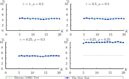
For the empirical size check, 10,000 replications are used. We report the results in Figures 1-4.
Firstly note that in both homoskedasticity and heteroskedasticity cases, the empirical size of the
new statistic is quite stable or becomes stable quickly as K increases. In the homoskedasticity case, its empirical size properties are comparable to Bierens (1990)’s statistic, even whenK = 3. In the heteroskedasticity case, under reasonable penalty parameters situations, while Bierens
(1990) statistic is undersized, the empirical size of the new statistic is a little bit undersized,
when K is a small number; it becomes very close to the nominal size, when K increases. Note that when penalty parameters are too small ({γ = 0.25, ρ= 0.25}), both statistics are all heavily oversized.
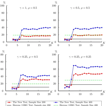
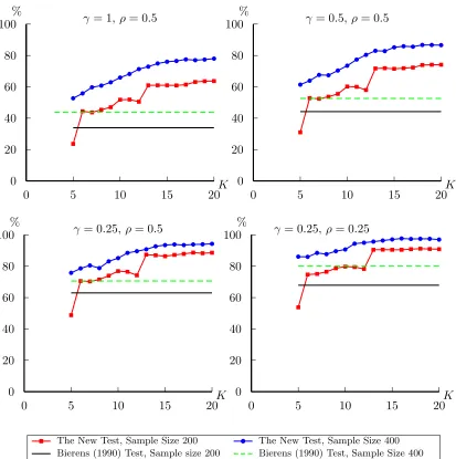
For the power check, 1000 replications are used. We consider the following alternatives
DGP 1.1: Y = 1 +X1+X2+v12v22+u.
DGP 1.2: Y = 1 +X1+X2+v12v22+ 0.1 + 0.5x21
1/2
u.
DGP 2.1: Y = 1 +X1+X2+ (1 +X1+X2) exp
h
−0.01 (1 +X1+X2)2
i +u.
DGP 2.2: Y = 1 +X1+X2+ (1 +X1+X2) exp
h
−0.01 (1 +X1+X2)2
i
+ 0.1 + 0.5x2 1
1/2
DGP 3.1: Y = 1 +X1+X2+ sin (1 +X1+X2) +u.
DGP 3.2: Y = 1 +X1+X2+ sin (1 +X1+X2) + 0.1 + 0.5x21
1/2
u.
DGP 4.1: Yj = 1 +X1+X2+ cos (1 +X1+X2) +u.
DGP 4.2: Yj = 1 +X1+X2+ cos (1 +X1+X2) + 0.1 + 0.5x21
1/2
u.
Remark: The second alternative is the same as the alternative 3 in Escanciano (2006a); The
third is similar to the alternative 4 in Escanciano (2006a). The fourth changes the sine function
in the third alternative into a cosine function.
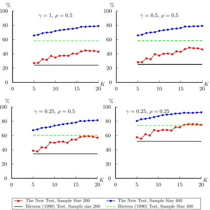
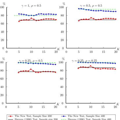
We report the results in Figures 5-12. To save space, results of sample size 200 and 400
are reported in one figure for each alternative. For the first alternative, our new statistic is
better than Bierens (1990)’s in both homoskedasticity and heteroskedasticity cases when K is relatively large. For the alternative 2, 3 and 4, under homoskedasticity, the power of the new
statistic is quite close to Bierens (1990)’s test for all the K we considered. In heteroskedasticity case, the new statistic has very good power properties even when K is small; as K increases, the difference of the power between the new statistic and Bierens (1990)’s test reaches as much
as 20%.
All in all, the new statistic has good size properties and improves the power significantly
when there exists heteroskedasticity of unknown form. The choice of K is not restrictive. For a large number of alternatives, the general pattern of the test results is that when K increases, we obtain better power properties.
9
Conclusion
In this paper, we have proposed a new consistent conditional test, combining the Bierens’
ap-proach and consistent test of overidentifying restrictions. It relies on a transformation-based
empirical process. The new empirical process enjoys some advantages of both approaches.
Firstly it is not affected by the uncertainty from the parameter estimation. Moreover This
estimation-effect-free property requires much less restrictive rate condition than in consistent
tests of overidentifying restrictions alone. Furthermore the ICM test based on the new empirical
process has power against Pitman local alternatives. We proved, under some regularity
condi-tions, the admissibility of the ICM test based on this transformation-based empirical process in
the case that there exists heteroskedasticity of unknown form, extending the result in Bierens
for future work.
Appendix
Proof of Corollary 1. Without loss of generality we may assume that X is bounded itself, so that we may choose Φ(X) =X. We set w(t′
1X) = 1. It is always possible to normalizeqK(X)
into this case when w(t′1X) 6= 1. Firstly it is easy to check that q(tjX) ∈ L2, for j = 1,2,· · ·.
For K= 2,3,· · ·, let
̟K(X) = K
X
j=1
αK,jw t′jX
,
where αK,K = 1, and the other αK,j are chosen such that
E̟K(X)w t′jX
= 0 if j < K.
For K= 1,2,· · ·, define function ψK(X) on the range of X such that
ψ1(X) = 1,
ψK(X) =
̟K(X)/E̟K(X)21/2, if E̟K(X)2>0
0, if E̟K(X)2
= 0
forK >1. ThenψK(X),K= 1,2,· · · form an orthonormal system of the Hilbert space ofHof
Borel measurable functions ϕon the range of X satisfyingEhϕ(X)2i<∞, with inner product (ψK, ϕ) =E[ψK(X)ϕ(X)]. Then by Theorem 2.4.2 of Brockwell and Davis (1991), for anyε,
there exists a positive integer K and constant c1,· · · , cK such that
E
ϕ(X)−
K
X
j=1
cjψj(X)
2
1/2
< ε,
Proof of Theorem 1. To prove this theorem, we rewrite ˜M(ˆθ, t, K) into
˜
M(ˆθ, t, K) = n−1/2
n
X
j=1
ρ(Zj,θˆ)w(t′Φ(Xj))
−ˆb(ˆθ, t) ˆAθ, Kˆ Λˆθ, Kˆ ′Ωˆθ, Kˆ −1n−1/2
n
X
j=1
qK(Xj)ρ(Zj,θˆ).
= A1−A2
By the mean value theorem we have
A1 =n−1/2
n
X
j=1
ρ(Zj, θ0)w(t′Φ(Xj)) + ˆb( ˙θ, t)n1/2
ˆ
θ−θ0
,
where ˙θ lies on the line joining ˆθ and θ0, ˙θ, θˆ∈ ∆, an open convex neighborhood of θ0, with
˙
θ →p θ0. By Assumption 4 and the fact that E[w2(t′Φ(X))] is finite, the dominance condition
holds by Cauchy-Schwarz inequality
E
sup
θ∈∆
w t′Φ(X)∂ρ(∂θZj′, θ)
=Ew t′Φ(X)sup
θ∈∆
∂ρ∂θ(Z, θ′ )
≤hEw t′Φ(X)2i1/2
"
Esup
θ∈∆
∂ρ(Z, θ)
∂θ′
2#1/2
<∞.
So we have weakly uniformly convergence of
plim sup
θ∈∆
1 n n X j=1
w t′Φ(X)∂ρ(Zj, θ0)
∂θ′ −E
w t′Φ(X)∂ρ(Z, θ)
∂θ′
= 0,
Following the Lemma 1 in Wang (2015), then ˆb( ˙θ, t)−ˆb(θ0, t) =op(1). So
A1 =n−1/2
n
X
j=1
ρ(Zj, θ0)w(t′Φ(Xj)) + ˆb(θ0, t)n1/2
ˆ
θ−θ0
Similarly
E
sup
θ∈∆
qK(X)∂ρ(∂θZ, θ′ )
=EqK(X)sup
θ∈∆
∂ρ(∂θZ, θ′ )
≤hEqK(X)2i1/2 "
Esup
θ∈∆
∂ρ(Z, θ)
∂θ′
2#1/2
<∞.
Then
plim sup
θ∈∆
1 n n X j=1
qK(X)∂ρ(Zj, θ)
∂θ′ −E
qK(X)∂ρ(Z, θ)
∂θ′
= 0, By similar argument, we have
n−1/2
n
X
j=1
ρ(Zj,θˆ)qK(Xj) =n−1/2 n
X
j=1
ρ(Z, θ0)qK(Xj) + ˆΛ(θ0, K)n1/2
ˆ
θ−θ0
+op(1),
Similarly
E
sup
θ∈∆
qK(X)qK(X)′[ρ(Z, θ)]2
=EqK(X)qK(X)′sup
θ∈∆
[ρ(Z, θ)]2
≤hEqK(X)qK(X)′2i1/2
Esup
θ∈∆
[ρ(Z, θ)]4 1/2
<∞.
Then by similar argument, ˆΩθ, Kˆ −Ω(ˆ θ0, K) =op(1). Also by Assumptions 4 and 5,
for any K > p, Ω(θ0, K) is positive definite. By continuous mapping theorem, for K > p,
ˆ
Λθ, Kˆ ′Ωˆθ, Kˆ −1Λˆθ, Kˆ −Λ(ˆ θ0, K)′Ω(ˆ θ0, K)− 1ˆ
Λ(θ0, K) =op(1), ˆΛ
ˆ
θ, K′Ωˆθ, Kˆ −1−
ˆ
Λ(θ0, K)′Ω(ˆ θ0, K)− 1
=op(1). Then
A2 = ˆb(θ0, t) ˆA(θ0, K) ˆΛ (θ0, K)′Ω (ˆ θ0, K)−1
×n−1/2
n
X
j=1
qK(Xj)ρ(Zj, θ0) + ˆΛ(θ0, K)n1/2
ˆ
θ−θ0
+op(1)
+op(1)
= ˆb(θ0, t) ˆA(θ0, K) ˆΛ (θ0, K)′Ω (ˆ θ0, K)−1n−1/2
n
X
j=1
qK(Xj)ρ(Zj, θ0)
+ˆb(θ0, t)n1/2
ˆ
θ−θ0
+op(1)
To prove (9), we rewrite ˜M(ˆθ, t, K) as
˜
M(ˆθ, t, K) = [1,−ˆb((θ0, t) ˆA(θ0, K) ˆΛ (θ0, K)′Ω (ˆ θ0, K)−1]n−1/2
n
X
j=1
ρ(Zj, θ0) w(t′Φ(Xj)), qK(Xj)′
′
+op(1).
(15)
By Lindberg-Feller central limit theory and Slutsky theorem, we have
˜
M(ˆθ, t, K)→d N0, s2(θ0, t, K)
Proof of Lemma 2. Denote ¯Ω (θ0, K) = 1nPni=1E ρ(Zi, θ)2|XiqK(Xi)qK(Xi)′. By applying
Lemma A.3 in Donald et al. (2003), ˆΛ (θ0, K)′Ω (¯ θ0, K)−1Λ (ˆ θ0, K) →p A∗(θ0)−1. By following
the proof of Theorem 5.4 in Donald et al. (2003), we can get ˆΛ (θ0, K)′Ω (¯ θ0, K)−1Λ (ˆ θ0, K)−
A(θ0, K)−1
p
→0.SoA(θ0, K)
p
→A∗(θ0).
By applying Lemma A.4 in Donald et al. (2003),
ˆ
Λ (θ0, K)′Ω (¯ θ0, K)−1n−1/2
n
X
j=1
qK(Xj)ρ(Zj, θ0)→p n−1/2
n
X
j=1
D(θ0, Xj)σ−2(θ0, Xj)ρ(Zj, θ0).
Also following the proof of Theorem 5.4 in Denald et al. (2003), we can get
ˆ
Λ (θ0, K)′Ω (¯ θ0, K)−1n−1/2
n
X
j=1
qK(Xj)ρ(Zj, θ0)−Λ (ˆ θ0, K)′Ω (ˆ θ0, K)−1n−1/2
n
X
j=1
qK(Xj)ρ(Zj, θ0)
p
→0.
Then
ˆ
Λ (θ0, K)′Ω (ˆ θ0, K)−1n−1/2
n
X
j=1
qK(Xj)ρ(Zj, θ0)
p
−n−1/2
n
X
j=1
D(θ0, Xj)σ−2(θ0, Xj)ρ(Zj, θ0)→0.
Proof of Theorem 2. Based on Lemma 2, it is easy to get
˜
M(ˆθ, t, K) =n−1/2
n
X
j=1
By Lindberg-Feller central limit theory
n−1/2
n
X
j=1
D(θ0, Xj)σ−2(θ0, Xj)ρ(Zj, θ0)→d N 0, A∗(θ0)−1
.
Then we can get
s2∗(θ0, t) =E
ρ(Z, θ0)2φ∗(θ0, X, t)2
Proof of Theorem 3. We need to show that the finite distributions of the process ˜M(ˆθ, t, K) con-verge to normal distributions, and that ˜M(ˆθ, t, K) is tight as K→ ∞ andξ(K)2K/n→0. The asymptotic normality of the finite distributions of ˜M(ˆθ, t, K) follows easily from the Liapunov-type version in Bierens (1994, Theorem 6.1.7) of McLeish’s (1974) martingale difference central
limit theorem. The tightness of ˜M(ˆθ, t, K) follows from Lemma A.1 in Bierens and Ploberger (1997). Denote Υ = supt∈T k∂w(t′Φ (X))/∂t′k. Firstly note E[Υ] ≤ EΥ4 1/4 < ∞, and
w(t′
1Φ(X)) is differentiable, so for any t1, t2 ∈ T,|w(t′1Φ(X))−w(t′2Φ(X))| ≤ Υ|t1−t2|.
Sec-ondly, Eρ(Z, θ0)2Υ2≤E1/2ρ(Z, θ0)4E1/2Υ4<∞. By continuous mapping theorem, we
get the asymptotic distribution of \ICMθ, Kˆ .
Proof of Theorem 5. Since e∗
i(ˆθ) =ei(ˆθ)Vi for 1≤i≤n, (12), it is easy to get
˜
M∗(ˆθ, t, K) =n−1/2
n
X
j=1
ρ(Zj, θ0)Vi[w(t′Φ(Xj))−ˆb(θ0, t) ˆA(θ0, K) ˆΛ (θ0, K)′Ω (ˆ θ0, K)−1qK(Xj)]
−n1
n
X
j=1
g(Xj) [w(t′Φ(Xj))−ˆb(θ0, t) ˆA(θ0, K) ˆΛ (θ0, K)′Ω (ˆ θ0, K)−1qK(Xj)] +op(1),
whenK → ∞andξ(K)2K/n→0. Then the conclusion follows similar to the proof of Theorem 4.
Proof of Lemma 3. We still assume thatX is bounded itself, so that we may choose Φ(X) =X. We set exp(t′1X) = 1. Note that we can always normalize qK(X) into qK(X) = (1,exp((t2−
t1)′X),· · · ,exp((tK−t1)′X))′. ForK = 1,2,· · ·, since the probability density function of X is
bounded away from zero, then the second moment of ̟K(X) defined in the proof of Lemma 1
is larger than zero, that isE̟K(X)2
>0 almost surely. So for K= 2,3,· · ·,
For any K, define ˜qK(X) = (ψ1(X),· · ·, ψK(X))′. When tjK 6= tiK for j, i = 1,· · · , K,
˜
qK(X) is linear transformation of qK(X): qK(X) = Bq˜K(X), where B is a nonsingular lower triangular matrix. So ˜qK(X) =B−1qK(X). Since (ψ
1(X),· · ·, ψK(X))′ is an orthonormal set,
soE q˜K(X) ˜qK(X)′=I
K, which means that the condition of nonsingularity is satisfied.
Note that||q˜K(X)||= [PK
j=1ψj(X)2]1/2,̟K(X) =PKj=1αK,jexp
t′
jX
, andXis bounded, So we have
sup
X∈U||
˜
qK(X)|| ≤C[
K
X
k=1
1]1/2
≤CK1/2.
To prove s2(θ0, t, K)>0, note that for anyt∈Π,t=6 tj for j= 1,· · · , K. DenoteqK+1(X) =
(exp(t′1Φ(X)),· · · ,exp(t′KΦ(X)),exp(t′Φ(X)))′. Then we can obtain thatE qK+1(X)qK+1(X)′ has smallest eigenvalue bounded away from zero based on Lemma 2. Note that E[(Y − f(X, θ0))|X]2 > 0, then E
(Yj−f(Xj, θ0))2qK+1(X)qK+1(X)′
is positive definite. From
(15) in the proof of Theorem 1 it is easy to obtain thats2(θ
0, t, K)>0.
Proof of Theorem 6. Under H0, Define
zn(θ0, t, K) = n−1/2
n
X
j=1
[Yj−f(Xj, θ0)][exp(t′Φ(Xj))
−ˆb(θ0, t) ˆA(θ0, K) ˆΛ (θ0, K)′Ω (ˆ θ0, K)−1qK(Xj)]/
p
(s2(θ0, t, K)).
Following the Proof of Theorem 1, we have under H0
p lim
n→∞supt∈Π|
˜
W(ˆθ, t, K)−zn2(θ0, t, K)|= 0.
Following the Proof of Lemma 4 in Bierens (1990), we can obtain underH0,zn(θ0, t, K) is tight.
Then We allowK → ∞, Kn2 →0, the following result holds
p lim
n→∞supt∈Π|
zn2(θ0, t, K)−z∗2(θ0, t)|= 0.
It is also easy to prove that for arbitrary t1,· · · , tm in Π, (zn(θ0, t1, K),· · · , zn(θ0, tm, K))′
References
[1] Bierens H.J., 1982. Consistent model specification test. Journal of Econometrics 20, 105-134.
[2] Bierens H.J., 1990. A consistent conditional moment test of functional form. Econometrica
58, 1443-1458.
[3] Bierens, H.J., Ploberger, W., 1997. Asymptotic theory of integrated conditional moment
tests. Econometrica 65, 1129-1152.
[4] Billingsley, P., 1968. Convergence of Probability Measures. New York: Wiley.
[5] Brockwell, P.J., Davis, R.A., 1991. Time Series: Theory and Methods (2nd Edition).
Springer.
[6] Chamberlain, G., 1987. Asymptotic efficiency in estimation with conditional moment
re-strictions. Journal of Econometrics 34, 305–334.
[7] Chamberlain, G., 1992. Comment: sequential moment restrictions in panel data. Journal
of Business and Economic Statistics 10, 20-26.
[8] Carrasco, M., Florens J.P., 2000. Generalization of GMM to a continuum of moment
con-ditions. Econometric Theory 16, 797-834.
[9] De Jong, R.M., 1996. The Bierens test under data dependence. Journal of Econometrics
72, 1-32.
[10] Dom´ınguez, M.A., Lobato,I.N., 2004. Consistent estimation of models defined by conditional
moment restrictions. Econometrica 72, 1601-1615.
[11] Dom´ınguez, M.A., Lobato,I.N., 2015. A Simple Omnibus Overidentification Specification
Test for Time Series Econometric Models. Econometric Theory 31, 891-910.
[12] Donald, G., Imbens, W., Newey, W.K., 2003. Empirical likelihood estimation and consistent
tests with conditional moment restrictions. Journal of Econometrics 117, 55-93.
[13] Escanciano, J.C., 2006a. A consistent diagnostic test for regression models using projections.
Econometric Theory 22, 1030-1051.
[14] Escanciano, J.C., 2006b. Goodness-of-fit statistics for linear and nonlinear time series
[15] Fan, Y., Li, Q., 1996. Consistent model specification tests: omitted variables and
semi-parametric functional forms. Econometrica 64, 865-890.
[16] Gozalo, P.L., 1993. A consistent model specification test for nonparametric estimation of
regression function models. Econometric Theory 9, 451-477.
[17] Hahn, J., 1997. Efficient estimation of panel data models with sequential moment
restric-tions. Journal of Econometrics 79, 1-21.
[18] H¨ardle, W., Mammen, E., 1993. Comparing nonparametric versus parametric regression
fits. The Annals of Statistics 21, 1926-1947.
[19] Hong, Y., White, H., 1995. Consistent specification testing via nonparametric series
regres-sion. Econometrica 63, 1133-1159.
[20] Mammen, E., 1993. Bootstrap and wild bootstrap for high-dimensional linear model. Annals
of Statistics 21, 225–285.
[21] Mcleish, D. L., 1974. Dependent Central Limit Theorems and Invariance Principles. Annals
of Probability, 2, 620-628.
[22] Newey, W.K., 1997. Convergence rates and asymptotic normality for series estimators.
Journal of Econometrics 79, 147–168.
[23] Stinchcombe, M., White, H., 1998. Consistent specification testing with nuisance
parame-ters present only under the alternative. Econometric Theory 14, 295-325.
[24] Stute, W., 1997. Nonparametric model checks for regression. The Annals of Statistics 25,
613-641.
[25] Stute, W., Thies, S., and Zhu, L. X., 1998. Model checks for regression: an innovation
process approach. The Annals of Statistics 26, 1916-1934.
[26] Stute, W., Gonzalez-Manteiga, W., and Presedo-Quindimil, M., 1998. Boot-strap
Approx-imations in Model Checks for Regression. Journal of the American Statistical Association,
93, 141–149.
[27] Wang, X., 2015. A general approach to conditional moment specification testing with
[28] White, H., 1994. Estimation, Inference and Specification Analysis. New York: Cambridge
University Press.
[29] Wu, C. F. J., 1986. Jacknife, Bootstrap and Other Resampling Methods in Regression
Analysis (with discussion). The Annals of Statistics, 14, 1261–1350.
[30] Zheng, J.X., 1996. A consistent test of functional form via nonparametric estimation
Figure 1: Size of testing at 5% level, Sample size 200,uj =ej 0 2 4 6 8 10
0 5 10 15 20
b b b b b b b b b b b b b b b b
%
K γ = 1,ρ= 0.5
0 2 4 6 8 10
0 5 10 15 20
b b b b b b b b b b b b b b b b
%
K γ = 0.5,ρ= 0.5
0 2 4 6 8 10
0 5 10 15 20
b b b b b b
b b b b b b b b b b
%
K γ = 0.25,ρ= 0.5
0 2 4 6 8 10
0 5 10 15 20
b b b b b b
b b b b b b b b b b
%
K γ = 0.25,ρ= 0.25
Bierens (1990) Test bb The New Test
Figure 2: Size of testing at 5% level, Sample size 400,uj =ej
0 2 4 6 8 10
0 5 10 15 20
b b b b b b b b b b b b b b b b
%
K γ = 1,ρ= 0.5
0 2 4 6 8 10
0 5 10 15 20
b b b b b b b b b b b b b b b b
%
K γ = 0.5,ρ= 0.5
0 2 4 6 8 10
0 5 10 15 20
b b b b b b b b b b b b b b b b
%
K γ = 0.25,ρ= 0.5
0 2 4 6 8 10
0 5 10 15 20
b b b b b b b b b b b b b b b b
%
K γ = 0.25,ρ= 0.25
[image:30.595.67.479.474.726.2]Figure 3: Size of testing at 5% level, Sample size 200,uj =
0.1 + 0.5x21j1/2ej
0 2 4 6 8 10
0 5 10 15 20
b b b b b b b b b
b b b b b b b
%
K γ = 1,ρ= 0.5
0 2 4 6 8 10
0 5 10 15 20
b b b b b b b b b
b b b b b b b
%
K γ = 0.5,ρ= 0.5
0 2 4 6 8 10
0 5 10 15 20
b b b b b b b b b
b b b b b b b
%
K γ = 0.25,ρ= 0.5
0 2 4 6 8 10
0 5 10 15 20
b b b b b b b b b b b b b b b b
%
K γ = 0.25,ρ= 0.25
[image:31.595.65.482.476.732.2]Bierens (1990) Test bb The New Test
Figure 4: Size of testing at 5% level, Sample size 400,uj =
0.1 + 0.5x21j1/2ej
0 2 4 6 8 10
0 5 10 15 20
b b b b b
b b b b b b b b b b b
%
K γ = 1,ρ= 0.5
0 2 4 6 8 10
0 5 10 15 20
b b b b b
b b b b b b b b b b b
%
K γ = 0.5,ρ= 0.5
0 2 4 6 8 10
0 5 10 15 20
b b b b b
b b b b b b b b b b b
%
K γ = 0.25,ρ= 0.5
0 2 4 6 8 10
0 5 10 15 20
b b
b b b b b b b b b b b b b b
%
K γ = 0.25,ρ= 0.25
Figure 5: Power of testing at 5% level, DGP 1.1 0 20 40 60 80 100
0 5 10 15 20
r
r
r
r
r
r r r r r r r r r r r r r
b
b b
b
b b b b b
b b b
b b b b b b
%
K γ = 1,ρ= 0.5
0 20 40 60 80 100
0 5 10 15 20
r
r
r
r
r
r r r r r r r r r r r r r
b
b b
b
b b b
b b b b b
b b b b b b
%
K γ = 0.5,ρ= 0.5
0 20 40 60 80 100
0 5 10 15 20
r
r
r
r
r
r r r r r r r r r r r r r
b
b b
b
b b b
b b b b b
b b b b b b
%
K γ = 0.25,ρ= 0.5
0 20 40 60 80 100
0 5 10 15 20
r
r
r
r
r r
r r r r r r r r r r r r
b b b b b b b
b b b b b b b b b b b
%
K γ = 0.25,ρ= 0.25
Bierens (1990) Test, Sample size 200 Bierens (1990) Test, Sample Size 400
Figure 6: Power of testing at 5% level, DGP 1.2
0 20 40 60 80 100
0 5 10 15 20
r
r r r
r
r r r r r r r r r r r r r
b b b
b
b b b b b b b b
b b b b b b
%
K γ = 1,ρ= 0.5
0 20 40 60 80 100
0 5 10 15 20
r
r r r
r r r r r r r r r r r r r r
b b b
b
b b b b b b b b b b
b b b b
%
K γ = 0.5,ρ= 0.5
0 20 40 60 80 100
0 5 10 15 20
r
r r
r
r r r r r r r
r
r r r r r r
b b b
b
b b b
b b b b b b b
b b b b
%
K γ = 0.25,ρ= 0.5
0 20 40 60 80 100
0 5 10 15 20
r
r r
r
r r r r r r r r r r r r r r
b
b
b
b
b b
b b b b b b b b b b b b
%
K γ = 0.25,ρ= 0.25
Bierens (1990) Test, Sample size 200 Bierens (1990) Test, Sample Size 400
Figure 7: Power of testing at 5% level, DGP 2.1
0 20 40 60 80 100
0 5 10 15 20
r r r r r r
r r r r r r
r r r r
b b b b b b b b b
b b b b b b b
%
K γ = 1,ρ= 0.5
0 20 40 60 80 100
0 5 10 15 20
r r r r r r
r r r r r r
r r r r
b b b b b b b b b
b b b b b b b
%
K γ = 0.5,ρ= 0.5
0 20 40 60 80 100
0 5 10 15 20
r r r r r r
r r r r r r r r r r b b b b b b b b b b b b b b b b
%
K γ = 0.25,ρ= 0.5
0 20 40 60 80 100
0 5 10 15 20
r r r r r r
r r r r r r r r r r
b b b b b b b b b b b b b b b b
%
K γ = 0.25, ρ= 0.25
Bierens (1990) Test, Sample size 200 Bierens (1990) Test, Sample Size 400
Figure 8: Power of testing at 5% level, DGP 2.2
0 20 40 60 80 100
0 5 10 15 20
r r r r
r
r r r r r r r
r r r r b b b
b b b b b
b b b b b b b b
%
K γ = 1,ρ= 0.5
0 20 40 60 80 100
0 5 10 15 20
r r r r
r r r r r r r
r r r r r
b b b b b
b b b b b b b b b b b
%
K γ = 0.5,ρ= 0.5
0 20 40 60 80 100
0 5 10 15 20
r r r r
r r r r r r r r
r r r r
b b b b
b b b b
b b b b b b b b
%
K γ = 0.25,ρ= 0.5
0 20 40 60 80 100
0 5 10 15 20
r r r r
r r r r r r r r
r r r r
b b b b
b b b b
b b b b b b b b
%
K γ = 0.25, ρ= 0.25
Bierens (1990) Test, Sample size 200 Bierens (1990) Test, Sample Size 400
Figure 9: Power of testing at 5% level, DGP 3.1
0 20 40 60 80 100
0 5 10 15 20
r r r r r
r
r
r r r r r r r r r
b b b b
b b b b b
b b b b b b b
%
K γ = 1,ρ= 0.5
0 20 40 60 80 100
0 5 10 15 20
r r r r r r r
r r r r r r r r r
b b b b
b b b b b b b b b b b b
%
K γ = 0.5,ρ= 0.5
0 20 40 60 80 100
0 5 10 15 20
r r r r r
r
r
r r r r r r r r r
b b b b b b b b b b b b b b b b
%
K γ = 0.25,ρ= 0.5
0 20 40 60 80 100
0 5 10 15 20
r r r r r
r
r
r r r r r r r r r
b b b b b b b b b b b b b b b b
%
K γ = 0.25, ρ= 0.25
Bierens (1990) Test, Sample size 200 Bierens (1990) Test, Sample Size 400
Figure 10: Power of testing at 5% level, DGP 3.2
0 20 40 60 80 100
0 5 10 15 20
r
r r r r r r r
r r r r r r r r
b b b b b
b b b b b
b b b b b b
%
K γ = 1,ρ= 0.5
0 20 40 60 80 100
0 5 10 15 20
r
r r r r r r r
r r r r r r r r
b b b b b
b b b b b
b b b b b b
%
K γ = 0.5,ρ= 0.5
0 20 40 60 80 100
0 5 10 15 20
r
r r r r r r
r
r r r r r r r r
b b b b b
b b b b b
b b b b b b
%
K γ = 0.25,ρ= 0.5
0 20 40 60 80 100
0 5 10 15 20
r
r r r r r r r
r r r r r r r r
b b b b b
b b
b b b b b b b b b
%
K γ = 0.25, ρ= 0.25
Bierens (1990) Test, Sample size 200 Bierens (1990) Test, Sample Size 400
Figure 11: Power of testing at 5% level, DGP 4.1
0 20 40 60 80 100
0 5 10 15 20
r r r r r r r r
r r r r r r r r
b
b
b b b
b b b b b b b b
b b b
%
K γ = 1,ρ= 0.5
0 20 40 60 80 100
0 5 10 15 20
r r r r r r r r
r r r r r r r r
b
b
b b b
b b b
b b b b
b b b b
%
K γ = 0.5,ρ= 0.5
0 20 40 60 80 100
0 5 10 15 20
r r r
r
r r r r r r r r
r
r r r
b
b
b b b
b b b b b b b b b b b
%
K γ = 0.25,ρ= 0.5
0 20 40 60 80 100
0 5 10 15 20
r r r
r
r r r r r r r r r r r r
b
b b b b
b b b b b b b b b b b
%
K γ = 0.25, ρ= 0.25
Bierens (1990) Test, Sample size 200 Bierens (1990) Test, Sample Size 400
Figure 12: Power of testing at 5% level, DGP 4.2 0 20 40 60 80 100
0 5 10 15 20
r r
r
r r
r
r r r
r r r r r r
r b b b b b b b b
b b b b b b
b b
%
K γ = 1,ρ= 0.5
0 20 40 60 80 100
0 5 10 15 20
r r
r
r r
r
r r r
r r r r r r
r b b b b b b b b
b b b b b b
b
b
%
K γ = 0.5,ρ= 0.5
0 20 40 60 80 100
0 5 10 15 20
r r
r
r r
r
r r r r r r r r r
r b b b b b b b b
b b b b
b b
b
b
%
K γ = 0.25,ρ= 0.5
0 20 40 60 80 100
0 5 10 15 20
r r
r
r r
r
r r r r r r r r r
r b b b b b b b b
b b b b b b
b
b
%
K γ = 0.25, ρ= 0.25
Bierens (1990) Test, Sample size 200 Bierens (1990) Test, Sample Size 400